


Introduction
Current planet formation theories predict that during or after the epoch of its formation a planet could be ejected from the hosting planetary system by interacting with a more massive planet (Lissauer Reference Lissauer1987), or with fly-by stars (Laughlin and Adams Reference Laughlin and Adams2000). The concept of starless planets has been introduced several decades ago, hypothesizing that some of them could host life (Shapley Reference Shapley1958, Reference Shapley1962; ÖPik Reference Öpik1964). Although Fogg (Reference Fogg1990) suggested their existence classifying them as ‘singular’ planets or ‘unbound’ planets, through decades their definition changed so that most of the studies now employs the term free-floating planetFootnote 1 (FFP).
Several attempts of direct observations of possible FFPs are reported (e.g. Zapatero Osorio et al. Reference Zapatero Osorio, Béjar, Martín, Rebolo, Barrado y Navascués, Bailer-Jones and Mundt2000; Liu et al. Reference Liu, Magnier, Deacon, Allers, Dupuy, Kotson, Aller, Burgett, Chambers, Draper, Hodapp, Jedicke, Kaiser, Kudritzki, Metcalfe, Morgan, Price, Tonry and Wainscoat2013; Luhman Reference Luhman2014; Liu et al. Reference Liu, Dupuy and Allers2016) and some of the potential candidates can be observed via microlensing techniques (Sumi et al. Reference Sumi, Kamiya, Bennett, Bond, Abe, Botzler, Fukui, Furusawa, Hearnshaw, Itow, Kilmartin, Korpela, Lin, Ling, Masuda, Matsubara, Miyake, Motomura, Muraki, Nagaya, Nakamura, Ohnishi, Okumura, Perrot, Rattenbury, Saito, Sako, Sullivan, Sweatman, Tristram, Yock, Szymanski, Kubiak, Pietrzynski, Poleski, Soszynski, Wyrzykowski and Ulaczyk2011; Bennett et al. Reference Bennett, Batista, Bond, Bennet, Susuki, Beaulieu, Udalski, Donatowicz, Bozza, Abe, Botzler, Freeman, Fukunaga, Fukui, Itow, Koshimoto, Ling, Masuda, Matsubara, Muraki, Namba, Ohnishi, Rattenbury, Saito To, Sullivan, Sumi, Sweatman, Tristram, Tsurumi, Wada, Yock, Albrow, Bachelet, Brillant, Caldwell, Cassan, Cole, Corrales, Coutures, Dieters, Dominis Prester, Fouqué, Greenhill, Horne, Koo, Kubas, Marquette, Martin, Menzies, Sahu, Wambsganss, Williams, Zub, Choi, DePoy, Dong, Gaudi, Gould, Han, Henderson, McGregor, Lee, Pogge, Shin, Yee, Szymański, Skowron, Poleski, Kozłowski, Wyrzykowski, Kubiak, Pietrukowicz, Pietrzyński, Soszyński, Ulaczyk, Tsapras, Street, Dominik, Bramich, Browne, Hundertmark, Kains, Snodgrass, Steele, Dekany, Gonzalez, Heyrovský, Kandori, Kerins, Lucas, Minniti, Nagayama, Rejkuba, Robin and Saito2014; Henderson Reference Henderson2016; Mróz et al. Reference Mróz, Ryu, Skowron, Udalski, Gould, Szymanski, Soszynsk, Poleski, Pietrukowicz, Kozlowski, Pawlak, Ulaczyk, Albrow, Chung, Jung, Han, Hwang, Shin, Yee, Zhu, Cha, Kim, Kim, Kim, Lee, Lee, Lee, Park and Pogge2018, Reference Mróz, Poleski, Han, Udalski, Gould, Szymanski, Soszynski, Pietrukowicz, Kozlowski, Skowron, Ulaczyk, Gromadzki, Rybicki, Iwanek, Wrona, Albrow, Chung, Hwang, Ryu, Jung, Shin, Shvartzvald, Yee, Zang, Cha, Kim, Kim, Kim, Lee, Lee, Lee, Park and Pogge2020). Theoretical estimates show that, on average, in our Galaxy there are two Jupiter-mass (Sumi et al. Reference Sumi, Kamiya, Bennett, Bond, Abe, Botzler, Fukui, Furusawa, Hearnshaw, Itow, Kilmartin, Korpela, Lin, Ling, Masuda, Matsubara, Miyake, Motomura, Muraki, Nagaya, Nakamura, Ohnishi, Okumura, Perrot, Rattenbury, Saito, Sako, Sullivan, Sweatman, Tristram, Yock, Szymanski, Kubiak, Pietrzynski, Poleski, Soszynski, Wyrzykowski and Ulaczyk2011; Clanton and Gaudi Reference Clanton and Gaudi2016) and 2.5 terrestrial-mass FFPs per star (Barclay et al. Reference Barclay, Quintana, Raymond and Penny2017), however, due to the uncertainty on mass, many candidates of FFPs can be classified either as planets or brown dwarves, assuming 13 MJ the mass threshold between the two classes (Caballero Reference Caballero2018).
These FFPs are capable of hosting moons. Debes and Sigurdsson (Reference Debes and Sigurdsson2007) showed that a relevant fraction of terrestrial-sized planets will likely to be ejected while retaining a lunar-sized companion. Exomoons less massive than their host companion are in principle detectable via transit timing variations (see e.g. Teachey et al. Reference Teachey, Kipping and Schmitt2018). The ‘Hunt for Exomoons with Kepler’ (HEK) project (Kipping et al. Reference Kipping, Bakos, Buchhave, Nesvorný and Schmitt2012) aims at searching these natural satellites using data collected by the Kepler space telescope. Despite the uncertainties related to the detection, Teachey and Kipping (Reference Teachey and Kipping2018) reported the evidence of a potential exomoon, although debated by other authors (Rodenbeck et al. Reference Rodenbeck, Heller, Hippke and Gizon2018; Heller et al. Reference Heller, Rodenbeck and Bruno2019; Kreidberg et al. Reference Kreidberg, Luger and Bedell2019). The microlensing event studied in Bennett et al. (Reference Bennett, Batista, Bond, Bennet, Susuki, Beaulieu, Udalski, Donatowicz, Bozza, Abe, Botzler, Freeman, Fukunaga, Fukui, Itow, Koshimoto, Ling, Masuda, Matsubara, Muraki, Namba, Ohnishi, Rattenbury, Saito To, Sullivan, Sumi, Sweatman, Tristram, Tsurumi, Wada, Yock, Albrow, Bachelet, Brillant, Caldwell, Cassan, Cole, Corrales, Coutures, Dieters, Dominis Prester, Fouqué, Greenhill, Horne, Koo, Kubas, Marquette, Martin, Menzies, Sahu, Wambsganss, Williams, Zub, Choi, DePoy, Dong, Gaudi, Gould, Han, Henderson, McGregor, Lee, Pogge, Shin, Yee, Szymański, Skowron, Poleski, Kozłowski, Wyrzykowski, Kubiak, Pietrukowicz, Pietrzyński, Soszyński, Ulaczyk, Tsapras, Street, Dominik, Bramich, Browne, Hundertmark, Kains, Snodgrass, Steele, Dekany, Gonzalez, Heyrovský, Kandori, Kerins, Lucas, Minniti, Nagayama, Rejkuba, Robin and Saito2014) could be interpreted as a free-floating exoplanet–exomoon system, however, they also point out that this is more probably a very-low-mass star with a Neptune-mass planet. Similarly, Fox and Wiegert (Reference Fox and Wiegert2021) suggested that some systems observed with Kepler are consistent with the presence of dynamically stable moons, but they also report that no definitive detection can be claimed on this basis, and therefore these systems will require further analysis. The detection limit is determined by the moon–planet mass ratio: for gas giants this is ~ 10−4 when formed together (e.g. in situ formation scenario), that corresponds to an upper limit of a Mars-sized moons (Canup and Ward Reference Canup and Ward2006), while this could reach Earth-sized objects if captured after a binary exchange encounter (Williams Reference Williams2013), depending on the size and the proximity of the planet and the host star, as well the velocity of the encounter.
The orbital parameters, the characteristics of the hosting star and the masses of the planet–moon system constrain the habitability of the moon (e.g. Heller et al. Reference Heller, Williams, Kipping, Limbach, Turner, Greenberg, Sasaki, Bolmont, Grasset, Lewis, Barnes and Zuluaga2014). In the case of a moon orbiting an FFP, the absence of stellar illumination suggests that the orbital parameters play the main role, since the orbital eccentricity determines the amount of tidal heating, a key energetic process that may favour the presence of life on the exomoon (Reynolds and Cassen Reference Reynolds and Cassen1978; Scharf Reference Scharf2006; Henning et al. Reference Henning, O'Connell and Sasselov2009; Heller Reference Heller2012; Heller and Barnes Reference Heller and Barnes2013a). In addition to that, the thermal budget of the exomoon could be controlled by the evolution of the incident planetary radiation (e.g. Haqq-Misra and Heller Reference Haqq-Misra and Heller2018), by the runaway greenhouse effect (Heller and Barnes Reference Heller and Barnes2014), and by processes like stellar radiation and thermal heat from the hosting planet (Dobos et al. Reference Dobos, Heller and Turner2017). Despite these models analyse in detail the role of the various thermal processes, they neglect the effect on the chemistry of the atmosphere, that needs to be considered to determine the conditions for the habitability (Lammer et al. Reference Lammer, Schiefer, Juvan, Odert, Erkaev, Weber, Kislyakova, Güdel, Kirchengast and Hanslmeier2014).
Although it has been discussed that an FFP with an atmosphere rich in molecular hydrogen could harbour life (Stevenson Reference Stevenson1999), it is paramount to model the chemical composition and evolution of CO2 and water to determine the opacity of the atmosphere that might allow liquid water on its surface. Badescu (Reference Badescu2010) analyses four gases (nitrogen, carbon dioxide, methane and ethane) as the main component of the FFP atmosphere to study the long-term thermal stability of a liquid solvent on the surface, and Badescu (Reference Badescu2011a, Reference Badescu2011b, Reference Badescu2011c) studied the possibility for an FFP to host life by calculating the thermal profiles and the solubility properties of condensed gas. It is also shown that these gases produces more effective opacities than H2, as originally suggested by Stevenson (Reference Stevenson1999).
Overall, these studies show that FFP and their moons might represent an environment compatible with the emergency of life within a wide range of masses and different atmospheric compositions, but, to the best of our knowledge, there are no detailed models of the chemical evolution of the atmosphere of a moon orbiting an FFP. Within this context, we introduce here an atmospheric model to tackle this limitation. We assume that in the absence of radiation from a companion star, the tidal and the radiogenic heating mechanisms represent the main sources of energy to maintain and produce an optimal range of surface temperatures. To model the thermal structure of the atmosphere of the exomoon orbiting around FFPs, we include these effects in a one-dimensional (1D) radiative-convective codeFootnote 2 (hereinafter named Patmo), alongside a gas-phase chemical kinetics network including cosmic rays, and ion–neutral and neutral–neutral chemistry. We evolve the system in order to determine the chemical evolution in time and the equilibrium time-scale to determine the total amount of water formed. Since an exhaustive definition of habitability represents a complicated issue (Lammer et al. Reference Lammer, Bredehöft and Coustenis2009), we limit ourselves to determine if liquid water is present on the surface of the exomoon (e.g. Kasting et al. Reference Kasting, Whitmire and Reynolds1993), while changing cosmic ray ionization, chemistry, temperature and pressure profiles of its atmosphere.
After describing the numerical methods to model the atmosphere we present our results. We then discuss the implications of our findings and future outlooks.
Methods
Planet–moon system
To model the dynamics of the planet–moon system, we assume that the FFP has been ejected from its host system by e.g. a perturbation from a gas giant planet, and it retained at least one of its moons after the ejection, as for example discussed in Debes and Sigurdsson (Reference Debes and Sigurdsson2007); Hong et al. (Reference Hong, Raymond, Nicholson and Lunine2018) and Rabago and Steffen (Reference Rabago and Steffen2019). The orbital parameters of the planet–moon system depend on the gravitational interaction during the ejection. Rabago and Steffen (Reference Rabago and Steffen2019) presented 77 simulations finding that 47% of the moons are likely to remain bond to the planet, and that the final semi-axis of a survived moon is <0.1 au (for comparison Jupiter's largest moons are within 0.01 au), but favouring the innermost orbits, as the number of moons is roughly inversely proportional to the final semi-axis a (namely, the probability of having a closer object after the ejection is higher). The final eccentricity e is mostly between 10−3 and 1 (Hong et al. Reference Hong, Raymond, Nicholson and Lunine2018). When present, the initial resonance is likely to survive the ejection, allowing the tidal heating to operate on longer time-scales compared to the case without resonances, i.e. 10 Myr according to Heller and Barnes (Reference Heller and Barnes2013a). The evolution in time of the orbital parameters determines the temporal domain of our model. In particular, the circularization of the orbit (e → 0) plays a key role in reducing the tidal heating produced on the moon by its interaction with the hosting planet, as it will be discussed more in detail in the Section ‘Thermal budget’ later in the text. For this reason 10 Myr represents the upper limit of the integration time of our atmospheric model.
We choose a range of semi-major axis and eccentricity following Debes and Sigurdsson (Reference Debes and Sigurdsson2007); Hong et al. (Reference Hong, Raymond, Nicholson and Lunine2018); Rabago and Steffen (Reference Rabago and Steffen2019), with the former ranging between 0.8 × 10⁻³ and 1.4 × 10⁻² au, while the latter between 10−3 and 5 × 10⁻¹. We assume a primary object (i.e. the FFP) with the mass of Jupiter, noting that the stability of the moon-planet system increases with the mass of the hosting planet.
To determine the mass of the moon orbiting around the FFP we follow Barnes and O'Brien (Reference Barnes and O'Brien2002) that indicate that a 1 M$_\oplus$ moon is stable when orbiting around a Jupiter-sized planet. Williams (Reference Williams2013) show that Earth-sized objects can be captured by a gas giant planet, thus leading to a massive satellite. Since such a planet–moon system could survive an ejection from their stellar system, as reported in the models of Rabago and Steffen (Reference Rabago and Steffen2019), we assume a configuration of a secondary object (i.e. the moon orbiting around the FFP) with a mass of 1 M$_\oplus$
 (and gravity g = 980 cm s−2) orbiting around a 1 MJ object, that allows to produce a significant amount of tidal heating to obtain liquid water when the atmosphere is not irradiated by any significant external radiation.
Atmospheric modelling
The chemical composition at different heights of a given exoplanet or exomoon atmosphere is determined by its interplay with the temperature and the vertical pressure profile. In fact, the temperature is driven by the opacity, a function of the chemical composition, while the chemical composition is affected by density and temperature. To model these processes and to predict the relevant quantities we employ Patmo, a code aimed at modelling 1D planetary atmospheres including (photo)chemistry, cosmic rays chemistry, molecular/eddy diffusion and multi-frequency radiative transfer. Patmo employs the dlsodes solver (Hindmarsh et al. Reference Hindmarsh, Brown, Grant, Lee, Serban, Shumaker and Woodward2009) to integrate in a full-implicit fashion a set of mass continuity equations:

where n i is the number density of the ith chemical species, t is the time, P i and L i are respectively the production and loss rates of the ith species, ϕ i its vertical transport flux and z is the cell altitude, where z = 0 represents the surface of the exomoon. We employ 100 linearly spaced cells ranging from z = 0 to 35 km and to 30 km, respectively for the low- and the high-pressure models (see Section ‘Results’). The vertical transport flux is

where K zz is the eddy diffusion coefficient, n tot the total number density and X i the mixing ratio of the ith species, that denotes the relative abundance of the ith species with respect to the total density, i.e. X i = n i/n tot. The system in equation (1) allows us to solve the time-dependent evolution of each species abundance n i, or when ∂t n i = 0 to find the equilibrium abundances.
As discussed later in this section, P i and L i are both functions of the vertical temperature profile, that is directly controlled by the optical depth τ. In principle, to determine the optical depth, we should track the evolution of the radiation when affected by a large number of molecular lines, that depend on the chemical composition and on the temperature, but this will be simplified by using an averaged opacity over the complete spectrum, i.e. a so-called grey opacity.
When τ is defined, the temperature of a non-irradiated atmosphere in a radiative thermal equilibrium can be expressed by (Marley and Robinson Reference Marley and Robinson2015)

that holds when the atmosphere is in the radiative regime, and where D = 1.5 is the diffusivity factor, τ is defined in order to be zero in the outermost layer of our modelled atmosphere and increases towards the surface, and T eff the effective temperature. The diffusivity factor ranges from 1.5 to 2 and depends on the geometrical details of the atmosphere, however, changing its value does not play any crucial role in our findings.
The black-body effective temperature follows the Stefan–Boltzmann law:

where $\dot {E}_{\rm total}$ is the total flux of energy (see ‘Thermal budget’ subsection), σsb is the Stefan–Boltzmann constant, εr = 0.9 is the infrared emissivity factor (Henning et al. Reference Henning, O'Connell and Sasselov2009) and R is the radius of the moon. The lower zone of the atmosphere is in the convective regime if (Sagan Reference Sagan1969; Weaver and Ramanathan Reference Weaver and Ramanathan1995; Robinson and Catling Reference Robinson and Catling2012)

where p is the pressure, $\nabla _{\rm ad}$ is the (dry) adiabatic lapse (i.e. the temperature vertical gradient) and γ is the adiabatic index, that depends on the chemical composition. If the atmosphere is in a convective regime, the relation between the pressure p and the temperature T is given by (Wallace and Hobbs Reference Wallace and Hobbs2006, p. 38)

where T r and p r are the temperature and the pressure evaluated at the boundary between the convective and the radiative regimes. Since by construction at the outermost layer of the atmosphere τ = 0, from equation (3) the temperature depends only on the effective temperature

We evaluate equation (5) with finite differences to determine if the atmosphere is in radiative or convective regime, applying equations (3) or (6) accordingly, i.e.

Opacity
The absence of external radiation suggests that a moon orbiting an FFP requires an optically thick atmosphere to prevent the loss of thermal energy and to keep a temperature that allows liquid water on its surface. In principle, the opacity of the atmosphere should be calculated dividing the radiation spectrum into several energy bins to cover the key spectral features of the chemical species involved. However, for our aims, this can be reasonably approximated by using an averaged mean opacity over the whole spectrum (Hansen Reference Hansen2008; Guillotm Reference Guillot2010; Robinson and Catling Reference Robinson and Catling2012; Parmentier and Guillot Reference Parmentier and Guillot2014). We decided to employ the Rosseland mean opacity because of the absence of stellar radiation, i.e.

where F(ν) is the weighting function and κv is the monochromatic opacity of a mixture of gases composed of N chemical species

where κν,i and q i are respectively the monochromatic opacity at a given frequency ν, and the mass-specific concentration of the ith species, with $\sum _{i = 1}^{N} q_i = 1$ . The weighting function is

where $B_\nu ( T)$ is the Planck spectral radiance at frequency ν of a black body with temperature T.
From the opacity we obtain the optical depth as a function of pressure:

where ρ a is the mass density of the atmosphere, g is the surface gravity of the moon, z top and p top are respectively the altitude and the pressure of the outermost layer, i.e. where τ = 0, and z|p is the altitude z corresponding to the pressure p. Once the grey opacity is known, we can compute the pressure-dependent temperature vertical profiles. To obtain the Rosseland mean we employ the opacity tables from Badescu (Reference Badescu2010), that have been specifically designed for FFPs. These values are valid from 50 to 647.3 K and for pressures between 10−5 and 2.212× 10² bar. Among the possible atmospheric chemical species that compose planetary atmospheres, we exclude N2 because of the small opacity (e.g. Badescu Reference Badescu2010), and molecular hydrogen and helium, since we assume that most of their mass has been lost over short time-scales via atmospheric escape, as it often happens in small bodies (Catling and Zahnle Reference Catling and Zahnle2009). Other species have higher opacity than molecular hydrogen (Stevenson Reference Stevenson1999; Badescu Reference Badescu2010), as for example methane, but planets formation theories indicate that a methane-based atmosphere is unlikely to exist (Pollack and Yung Reference Pollack and Yung1980; Lammer et al. Reference Lammer, Schiefer, Juvan, Odert, Erkaev, Weber, Kislyakova, Güdel, Kirchengast and Hanslmeier2014; Massol et al. Reference Massol, Hamano, Tian, Ikoma, Abe, Chassefière, Davaille, Genda, Güdel, Hori, Leblanc, Marcq, Sarda, Shematovich, Stökl and Lammer2016; Lammer et al. Reference Lammer, Zerkle, Gebauer, Tosi, Noack, Scherf, Pilat-Lohinger, Güdel, Grenfell, Godolt and Nikolaou2018). Ammonia, that has been for example proposed to be the origin of Titan's N2 (Glein Reference Glein2015), and it has been observed on the Saturnian moons, but not on the Jovian ones (Clark et al. Reference Clark, Swayze, Carlson, Grundy and Noll2014; Nimmo and Pappalardo Reference Nimmo and Pappalardo2016), could also play a role as an additional opacity term (e.g. Kasting Reference Kasting1982). Since the amount of ammonia depends on the moon's formation history (e.g. Mandt et al. Reference Mandt, Mousis, Lunine and Gautier2014), in our case we assume that CO2 alone controls the thermal evolution of an FFP atmosphere as it happens in our Solar System, and we therefore employ it in our model, assuming γ = 1.3 (Robinson and Catling Reference Robinson and Catling2012).
Thermal budget
The total energy flux in equation (4) is the sum of the tidal and radiogenic heating terms

The global heat tidal generation rate $\dot {E}_{\rm tidal}$ of a spin-synchronous homogeneous body on an eccentric orbit, assuming that its stiffness and dissipation are constant and uniform in time, reads (Murray and Dermott Reference Murray and Dermott2000; Henning et al. Reference Henning, O'Connell and Sasselov2009)

where k 2 is the second-order Love number of the satellite (secondary body), G is the gravitational constant, M p is the mass of the planet (primary body), R s is the radius of the satellite, n is the mean orbital motion, e is the eccentricity, Q is the quality factor of the satellite and a is the semi-major axis. The masses and radii of the bodies can be determined from planetary formation simulations and from available exoplanetary data. The eccentricity and the semi-major axis are free parameters in our models. In contrast, k 2 and Q depend on the material properties, specifically on the complex internal deformation processes. By definition (Murray and Dermott Reference Murray and Dermott2000; Henning et al. Reference Henning, O'Connell and Sasselov2009),

where $\bar {\mu }$ is the effective rigidity of the body defined as

where μ is the material rigidity and ρs is the mass density of the satellite. We assume common values for rocky bodies, μ = 5 × 10¹¹ dyne cm−2 and Q = 100 (Yoder and Peale Reference Yoder and Peale1981).
The tidal heating, as modelled in equation (14), depends on the orbital parameters and consequently on their evolution in time. However, in our model we assume that these parameters are constant, but we expect that the circularization of the orbit (e → 0) will reduce the total amount of heating in ~10 Myr (Heller and Barnes Reference Heller and Barnes2013a). For this reason we limit the time-scale of our models to 10 Myr, and we plan to discuss the coupling of the orbital parameters evolution with the atmospheric modelling in a forthcoming study.
The radiogenic heating is determined by the abundances of the radioactive sources similar to those of Earth, hence, we scale it to the total mass of the moon following Henning et al. (Reference Henning, O'Connell and Sasselov2009). The internal heat flux for the Earth is estimated between 3 × 10²⁰ and 4.6 × 10²⁰ erg s−1 (Jaupart et al. Reference Jaupart, Labrosse and Mareschal2007). About half of this heat, around 2.4 × 10²⁰ erg s−1 (Dye Reference Dye2012), is originated by radioactive decay, while the rest corresponds to other minor sources, including residual formation heat. Although the heat flux could be higher at early times, about nine times in the early Earth (Henning et al. Reference Henning, O'Connell and Sasselov2009), we include radiogenic heating for the sake of completeness, but we note that in our models tidal heating is the dominant factor, being at most 2 orders of magnitude larger than the radiogenic heating.
Low-temperature chemistry
The amount of heating produced by the tidal forces, and maintained by the optically thick atmosphere, produces a relatively low-temperature environment, i.e. below 300 K (see Section ‘Results’), and for this reason we limit our chemical network to include the reactions that are effective in this specific temperature range.
We use a reduced version of the STAND2015 chemical network (Rimmer and Helling Reference Rimmer and Helling2016), assuming that photochemistry is not relevant, since by definition an FFP and its satellite do not receive any significant radiation from any companion star. The STAND2015 Atmospheric Chemical Network contains H-, C-, N- and O-based chemical compounds and He, Na, Mg, Si, Cl, Ar, K, Ti and Fe atoms (necessary in their models for high-temperature chemistry, e.g. lightning). Since in our case we are interested in a low-temperature environment, we limit our study to reactions including molecules formed by H, C and O atoms only. We reduced the total number of species to 101, similarly to Tsai et al. (Reference Tsai, Lyons, Grosheintz, Rimmer, Kitzmann and Heng2017), and added the reverse rates that are relevant in our temperature range. We also discarded every two-body reaction with a rate constant smaller than 10−15 cm3 s−1 at 300 K and three-body reactions which are only active at temperatures above the ones considered in this study. For the sake of completeness, from KIDA databaseFootnote 3 (Wakelam et al. Reference Wakelam, Loison, Herbst, Pavone, Bergeat, Béroff, Chabot, Faure, Galli, Geppert, Gerlich, Gratier, Harada, Hickson, Honvault, Klippenstein, Le Picard, Nyman, Ruaud, Schlemmer, Sims, Talbi, Tennyson and Wester2015) we included cosmic rays reactions not present in STAND2015, but that involve the species in the network. The final network consists of 790 reactions, including three-body, ion-molecule and cosmic rays chemistry. Patmo has been benchmarked with the publicly available code vulcan (Tsai et al. Reference Tsai, Lyons, Grosheintz, Rimmer, Kitzmann and Heng2017), providing a perfect matching of the chemical vertical profiles. These tests and the chemical network are available in the code repositoryFootnote 4 .
Cosmic-ray chemistry
Since photochemistry is not included, the main ionization drivers are cosmic rays, that consequently determine the indirect formation and the direct destruction of the key molecular species. Cosmic-ray dissociation and ionization are parameterized by using the cosmic-rays ionization rate (CRIRFootnote 5) ζ, and we follow Rimmer and Helling (Reference Rimmer and Helling2013) to compute the atmospheric attenuation of the impinging interstellar cosmic rays from the outermost layer:

where ζj is the CRIR on the jth atmospheric layer, ζ0 the non-attenuated flux (i.e. z → ∞), σ the collisional averaged cross-section and N j the column density obtained integrating the total density from the outermost layer of the atmosphere down to the jth layer. We employ σ = 10−25 cm2 (Molina-Cuberos et al. Reference Molina-Cuberos, Lichtenegger, Schwingenschuh, López-Moreno and Rodrigo2002), and to mimic the different locations of the hosting planet in the Galaxy, we vary the CRIR between 10−17 and 10−12 s−1, the latter value to study the effects of a considerably stronger and somewhat extreme case. We also note that this value could be further reduced from the shielding of the magnetosphere of the hosting planet, as found for example in the Jupiter–Europa system (Nordheim et al. Reference Nordheim, Jasinski and Hand2019), or as discussed in the time-dependent model by Heller and Zuluaga (Reference Heller and Barnes2013b). These studies suggest that in some cases the presence of magnetic fields plays a crucial role in determining the amount of cosmic rays (and charged particle in general) impinging the atmosphere of the exomoon, affecting the position of the ‘habitable edge’, i.e. the minimum circumplanetary orbital distance, at which the moon becomes uninhabitable (Heller and Barnes Reference Heller and Barnes2013a).
Results
Thermal profiles
We compute the thermal profile for our atmosphere by employing equation (8) and assuming radiative thermal equilibrium throughout our study. The temperature on the moon surface (T 0) depends on the effective temperature T eff (a function of the orbital parameters) and on the surface pressure p 0. In Fig. 1 we show how T eff is affected by the semi-major axis (a) and the eccentricity (e); the left top panel shows the effective temperature T eff, i.e. the airless moon without the atmosphere, while the other panels show the surface temperature for different surface pressure values, assuming the opacity of a CO2-dominated atmosphere. We note that the isothermal regions follow a power-law relation between a and e (as shown by the black reference lines in Fig. 1). In particular, from equation (14) expanding the mean motion n in terms of a and e, we obtain

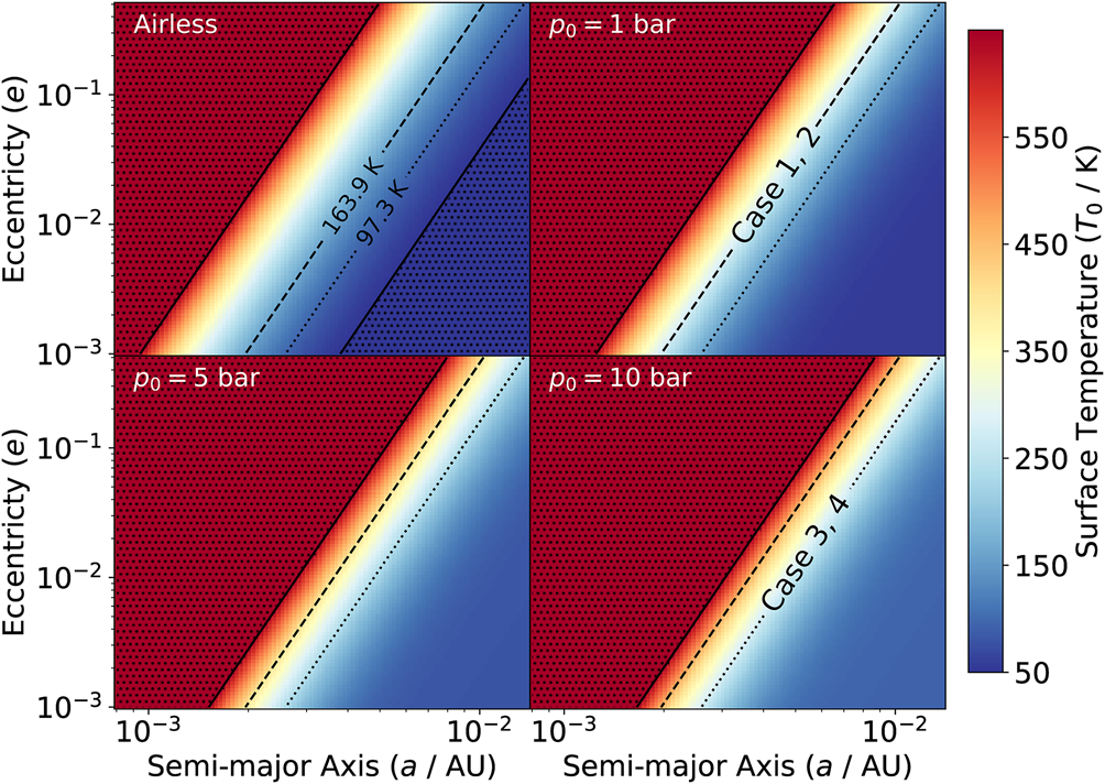
Fig. 1. Surface temperature of a satellite with 1 M$_\oplus$ , orbiting around a planet of 1 MJ. Eccentricity (e) ranges between 10−3 and 5 × 10⁻¹, while semi-major axis (a) between 0.8 × 10⁻³ and 1.4 × 10⁻² au. Left top panel: the satellite has no atmosphere (airless body), hence T 0 = T eff. Other panels: same as the first panel, but for different surface pressures p 0 assuming a CO2-dominated atmosphere. As a reference, the dotted and dashed lines are isothermal contours at respectively T eff = 97.3 and 163.9 K assuming the values of the first panel. The latter effective temperature corresponds to a surface temperature of 274.5 K in models Case1 and Case2, and analogously, the former, in models Case3 and Case4. The upper and the lower bounds of the colourbar are determined by the limits of the opacity tables, namely 50 and 647.3 K. The area outside these limits is indicated by the dotted hatch.
Since increasing p 0 globally increases the surface temperature, for operational purposes we choose a specific pressure rather than selecting eccentricity and semi-major pairs to obtain different temperatures, and for this reason in our models we change only p 0 (and consequently T eff), instead of varying a and e. Note that same (p, T 0) pairs correspond to multiple (a, e) pairs, suggesting a degeneracy between the orbital parameters and the atmospheric properties (i.e. different combinations of orbital parameters lead to the same atmospheric properties). This degeneracy is apparent, being determined by the time-independent modelling of the orbital parameters a and e, and therefore it represents only an operational method to reduce the number of atmospheric models and to have a clearer discussion of our results. However, in future studies, where the chemical-atmospheric model will be evolved alongside the orbital parameters, this apparent degeneracy will be removed by construction.
Our parameter space is represented by four limiting cases with two different surface pressure values (1 and 10 bar) and two different cosmic rays fluxes, namely, low (1.3 × 10⁻¹⁷ s−1) and high (10−12 s−1), as reported in Table 1. Our choice of parameters guarantees a surface temperature for which water is liquid, i.e. in each case we always obtain T 0 ~ 274.5 K, that corresponds to 1.35 times the freezing point in our pressure range. The two different atmospheric configurations of our 1 M$_\oplus$ exomoon are determined by its formation history and the subsequent evolution (Lammer et al. Reference Lammer, Zerkle, Gebauer, Tosi, Noack, Scherf, Pilat-Lohinger, Güdel, Grenfell, Godolt and Nikolaou2018), and for this reason the mass of the moon has no direct influence on the mass of its atmosphere and on the pressure at the surface, as shown for example by comparing the Earth (p = 1 $p_\oplus$
 , m = 1 M$_\oplus$
 ), Venus (91 $p_\oplus$
 , 0.82 M$_\oplus$
 ) and Titan (1.5 $p_\oplus$
 , 0.02 M$_\oplus$
 ). We therefore assume that the two values employed for the surface pressure are plausible and that are unaltered during the simulation. The lower limit of the cosmic rays flux is typically used in the dense interstellar medium (Dalgarno Reference Dalgarno2006). The upper limit represents an extreme case found in the interstellar gas nearby a gamma-ray-emitting supernova remnants (Becker et al. Reference Becker, Black, Safarzadeh and Schuppan2011). Although this extreme value reproduces a very specific environment, we choose this as an upper limit that allows to compare the effects of the atmospheric attenuation on the chemistry in the high-pressure cases.
Table 1. Parameter space explored in this study

The surface temperature T 0 in every case is 274.5 K. The last three columns indicate the case description employed in the text for pressure, cosmic rays ionization and temperature, e.g. Case1 is low-pressure, low-CRIR and high-temperature.
Since we ignore the heating from cosmic rays, being at most an order of magnitude smaller than the radiogenic heating, the vertical thermal profiles reported in Fig. 2 depend only on p 0. The left panel of Fig. 2 shows the variation of the temperature with pressure (and hence with height) for two models with two different ground pressures (p 0), but with the same ground temperature (T 0). For this reason in both cases the two thermal profiles guarantee liquid water on the surface. The vertical thermal profiles are obtained from equation (3) and equation (7) by constraining the effective temperature T eff, with the optical depth in equation (3) computed from equation (12) by constraining the surface pressure p 0. In our model the thermal profiles do not change in time, since we assume that the heating sources are constant, and that the atmosphere is always in hydrostatic equilibrium, i.e. readjustments of the vertical density profile are instantaneous.
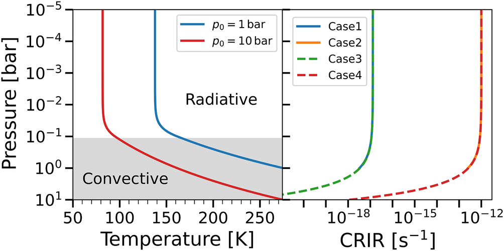
Fig. 2. Left panel: vertical thermal profiles for p 0 = 1 bar (Case1 and Case2) and 10 bar (Case3 and Case4). The surface temperature T 0 = 274.5 K is the same in both cases. Thermal profiles are assumed to be constant with time and independent from the CRIR. The grey-shaded area indicates the convective regime. Right panel: CRIR as a function of the vertical pressure. Note that Case1 (solid blue) and Case3 (dashed green) as well as Case2 (solid orange) and Case4 (dashed red) overlap, since the non-attenuated ionization rate is the same. The higher pressure reached by Case3 and Case4 allows the cosmic rays to penetrate deeper in the atmosphere, but with a larger attenuation when reaching the surface.
The optical depth found in our profiles increases from the outermost layers of the atmosphere (τ = 0) reaching τ = 50.33 at 1 bar, and τ = 4767.57 at 10 bar. For $p\gtrsim 10^{-4}$ bar this can be generalized with the power-law τ(p) = 50.33 p 1.97, where the pressure p is in units of bar.
In the right panel of Fig. 2 we report the vertical profile of the CRIR, for the different models. We note that the attenuation depends on the unaffected ionization, i.e. ζ0, and the depth of the atmosphere (i.e. the pressure reached at the surface). In fact, in the high-pressure models (Case3 and Case4, surface at p = 10 bar) the cosmic rays penetrate deeper in the atmosphere, but their attenuation on the surface is larger when compared to the low-pressure models (Case1 and Case2, surface at p = 1 bar). In terms of CRIR, the right panel of Fig. 2 also indicates that Case3 (Case4) represents an extension of Case1 (Case2), where the cosmic rays reach higher-pressure layers.
All the models assume that the atmosphere of the moon is initially vertically uniform and composed of 90% CO2 and 10% H2 (in number density), following a scenario where carbon dioxide is generated by evaporation from rocks, and locked there during the solidification phase when the body was still forming (Pollack and Yung Reference Pollack and Yung1980; Lebrun et al. Reference Lebrun, Massol, ChassefièRe, Davaille, Marcq, Sarda, Leblanc and Brandeis2013; Lammer et al. Reference Lammer, Schiefer, Juvan, Odert, Erkaev, Weber, Kislyakova, Güdel, Kirchengast and Hanslmeier2014; Massol et al. Reference Massol, Hamano, Tian, Ikoma, Abe, Chassefière, Davaille, Genda, Güdel, Hori, Leblanc, Marcq, Sarda, Shematovich, Stökl and Lammer2016; Lammer et al. Reference Lammer, Zerkle, Gebauer, Tosi, Noack, Scherf, Pilat-Lohinger, Güdel, Grenfell, Godolt and Nikolaou2018). Under our assumptions molecular hydrogen is a key ingredient for the formation of water, being the initial reservoir of hydrogen, and unlike warmer planets that are known to lose H2 over relatively short periods because of the thermal escape (Catling and Zahnle Reference Catling and Zahnle2009), a moon with a cold environment could retain a fraction of molecular hydrogen consistent with the abundances employed in this study (Stevenson Reference Stevenson1999). This initial abundance of molecular hydrogen is not relevant to affect the opacity, but crucial for the formation of water.
Time evolution of water formation
We evolve the chemistry in time for 10 Myr according to equation (1) and we report in the left panel of Fig. 3 the total amount of water integrated over all layers. In particular, from the water mixing ratio of each layer $x_{{\rm H_2O}, i}$ we compute the total mass of water produced in the atmosphere as ${M_{\rm H_2O} = \mu _{\rm H_2O}\sum _i\Delta V_i n_{{\rm tot}, i} x_{{\rm H_2O}, i}}$
 , where the sum is over every layer, $\Delta V_i = 4\pi ( \hat z_{i + 1}^{3} - \hat z_i^{3}) /3$
 is the volume of the ith layer, n tot,i its total number density, $\mu _{\rm H_2O}$
 the mass of a water molecule and $\hat z_i = z_i + R_{\rm s}$
 , i.e. the altitude including the radius of the exomoon. Analogously, the total mass of the atmosphere is ${M_{\rm tot} = \sum _i\mu _i\Delta V_i n_{{\rm tot}, i}}$
 , where μi is the mean molecular weight computed in the ith layer.

Fig. 3. Left panel: evolution of the vertically integrated fraction of water relative to the total mass of the atmosphere, for the models reported in Table 1 as a function of time. Case1 (blue) corresponds to high-temperature, low-pressure, low-CRIR; Case2 (orange) high-temperature, low-pressure, high-CRIR; Case3 (green) low-temperature, high-pressure, low-CRIR; Case4 (red) low-temperature, high-pressure, high-CRIR. The atmosphere is initially composed of 90% CO2 and 10% H2. Right panel: cumulative mass of water at 10 Myr integrated from the surface as a function of the pressure, i.e. the ith layer has ${f_i = \sum _{j = 1}^{i}M_{{\rm H_2O}, j} / M_{\rm tot}}$ . Note that for Case1 and Case2 the surface pressure is p 0 = 1 bar, while p 0 = 10 bar for Case3 and Case4.
The total amount of water formed in Case1 and Case2 is respectively ${M_{\rm H_2O} = 1.32\times 10^{17}}$ kg (at $t\gtrsim 100$
 Myr) and 1.24 × 10¹⁷ kg ($t\gtrsim 100$
 years), while for Case3 and Case4 is 2.85 × 10¹⁷ kg and 1.27 × 10¹⁸ kg (both at t ≃ 10 Myr), respectively. For comparison, the total mass of water in the Earth's oceans is ~ 1.4 × 10²¹ kg (Weast Reference Weast1979). The total corresponding atmospheric mass is M tot = 5.02 × 10¹⁸ kg (Case1 and Case2) and M tot = 4.93 × 10¹⁹ kg (Case3 and Case4). Again, for comparison, the mass of the Earth's atmosphere is 5.15 × 10¹⁸ kg (Trenberth and Smith Reference Trenberth and Smith2005).
The cumulative contribution to the total mass of water at the end of the simulation integrated from the surface layer as a function of the pressure is reported in the right panel of Fig. 3. For Case1 and Case2 the surface layers ($p\gtrsim 0.1$ bar) comprise almost the total mass of water present in the atmosphere. Analogously, Case3 and Case4 reach almost the total mass of water at ~1 bar, even if Case3 is far from the chemical equilibrium (see left panel of Fig. 3).
In Fig. 3 all the models have a steady increase of the fractional water content over time (note the logarithmic scale), followed by a relative reduction of the formation rate (and in some cases an equilibrium plateau) that depends on the amount of CRIR and on the temperature profile of the specific model. The final fractional amount of water is similar in each model, but reached with different time-scales. A shorter time-scale is found in the models with higher CRIR, i.e. Case2 and Case4, being the cosmic rays attenuation by the atmosphere ineffective and thus leading to a faster chemistry, mainly due to the dissociation of the initial reservoir of CO2 and H2. In these models, the chemical kinetic driven by the cosmic rays is effective in every layer, including the deeper ones. The less prominent plateau of the high-pressure Case4 is caused by the missing contribution of the deeper layers, where the CRIR is comparably less effective (see Fig. 2). Conversely, in Case1, where the CRIR efficiency is smaller, the equilibrium time-scale for water is considerably longer, being around 107 years, and in the high-density Case3 the equilibrium is not reached even within the simulation time. This slower (and not CRIR-driven) evolution is mainly controlled by the low-temperature chemistry, which is less effective when compared for example to Earth.
The stability observed in Case2 (but also in Case1 and Case4) is mainly due to the balance between the formation channel H2 + OH → H2O + H and the destruction reaction H2O + CR → OH + H (where CR indicates that the reactant interacts with cosmic rays), as discussed in detail in Section ‘Chemical vertical profiles’. This scenario might be altered in the surface layer by the destruction of water driven by condensation/rain-out processes, i.e. the removal from the gas phase (Hu et al. Reference Hu, Seager and Bains2012), but this process is not included in the present model.
The opacity of the atmosphere is controlled by CO2, the initial oxygen reservoir. This is mainly eroded by the CRIR-driven dissociation reaction CO2 + CR → CO + O, efficiently balanced by the formation routes CO + OH → CO2 + H and (less relevant) O + HCO → CO2 + H. Since these formation processes are effective during the evolution of every model, CO2 remains relatively constant in time when compared to water, that never becomes dominant over carbon dioxide, causing our approximation of a CO2-dominated atmosphere to hold. Nevertheless, water contributes to the total opacity, as reported by Lehmer et al. (Reference Lehmer, Catling and Zahnle2017), that explored water-dominated atmospheres of moons around gas giant planets. Even if CO2 is partially replaced with water, due to the high optical depth, the lower part of the atmosphere remains in a convective regime (see Fig. 2), and the surface remains warm enough to have liquid water. For comparison, on the Earth (around 10−3 bar and 220 K) the rotation bands of water vapour play a role for wavelengths $\gtrsim \!20$ μm and $\lesssim \!7.5$
 μm, while CO2 is known to reduce the escaping radiation flux around 15 μm, where H2O is less efficient (Zhong and Haigh Reference Zhong and Haigh2013).
Chemical vertical profiles
Our code not only allows to compute the evolution of the total abundances, but also their vertical profiles as reported in Fig. 4 for the four cases at 107 years and for different chemical species (note that e.g. Case2 reaches this profile after 102 years already, see Fig. 3). As previously discussed, water abundance is determined by the main formation channel H2 + OH → H2O + H that reaches equilibrium with H2O + CR → OH + H. The oxygen necessary for the formation of OH, is produced by the reaction CO2 + CR → CO + O, i.e. controlled by the efficiency of cosmic rays to penetrate the atmosphere of the exomoon (cf. Fig. 2). In fact, Case3 is the only model presenting a significant variation of water abundance in the surface layers. This specific model has low-CRIR (as Case1) and a denser atmosphere (as Case4), hence the chemistry is affected by the noticeably effective CRIR attenuation.
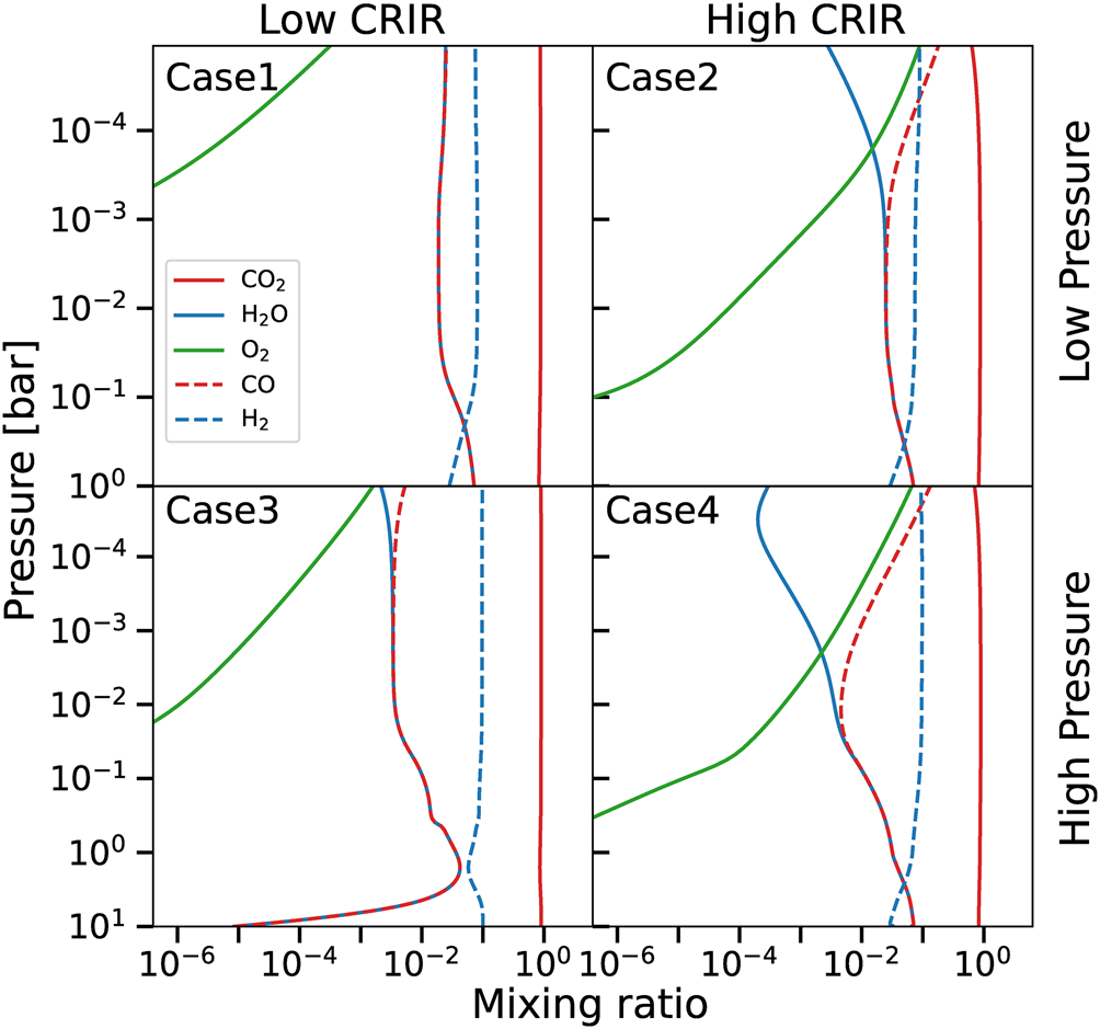
Fig. 4. Vertical distribution of different chemical species for an atmosphere composed of 90% CO2 and 10% H2 at 107 years. Upper panels correspond to high temperature and low pressure, lower panels to low temperature and high-pressure cases. Leftmost panels are lower cosmic rays ionization, while rightmost panels higher cosmic rays ionization models. Lines indicate CO2 (solid red), water (solid blue), molecular oxygen (solid green), CO (dashed red) and H2 (dashed blue).
The reduced amount of water in the upper part of the atmosphere in the high-CRIR models (Case2 and Case4) is determined by the more efficient destruction by CRIR. The difference between these two cases is enhanced by the corresponding temperature profiles, since the reaction H2 + OH → H2O + H is more efficient at higher temperatures, i.e. Case2 produces more water being comparably warmer, see Fig. 2.
In the lower layers of every model the presence of the three-body reaction H + CO + M → HCO + M (where M is a catalysing species) is the starting point of an additional route for the formation of water. In fact, it favours the formation of CH2O, via HCO + HCO → CH2O + CO, that reacts with H3O+ to form water by ${\rm CH_2O\ + \ H_3O^{ + }\to CH_3O^{ + }\ + \ H_2O}$ , this one balanced by its reverse reaction. This process is ineffective in the upper layers, due to the relatively low density that reduces the effectiveness of the aforementioned three-body reaction.
The reservoir of CO2 remains almost unaltered during the evolution, apart from the tiny variations in the upper layers of the high-CRIR cases (Case2 and Case4 in Fig. 4). Carbon dioxide chemistry is mainly controlled by the cosmic-rays driven destruction channel CO2 + CR → CO + O, effectively balanced by CO + OH → H + CO2, and by two minor formation reactions that involve oxygen, namely HCO + O → CO2 + H and HCO + O2 → CO2 + OH. Note that the oxygen produced by the CRIR dissociation of CO2 determines the formation of OH, a key ingredient for the formation of water.
Carbon dioxide and water formations compete for OH, respectively via CO + OH → CO2 + H and H2 + OH → H2O + H. Both CO and OH are formed via the destruction of CO2 and H2O by CRIR, thus obtaining two groups of balanced reactions linked by OH. This explains the pressure-dependent behaviour of CO and water (more pronounced in the high-CRIR cases), that closer to the surface present the same abundances, while in the upper layers CO becomes the dominating species. In particular, in the upper layers the higher CRIR and the lower densities enhance the formation of CO and the destruction of water. This effect is further enhanced by the lower temperatures of the high-pressure cases, that reduce the effectiveness of the formation of water (cf. the upper layers of Case1 with Case3 and Case2 with Case4).
Molecular oxygen presents a clear vertical gradient, determined by O2 + O + M → O3 + M, a three-body reaction, and O3 + HCO → CO2 + O2 + H, that both play a role in the lower layers of every model, with their efficiency controlled by the different temperature gradients, and by the availability of oxygen from the CO2 CRIR dissociation.
Molecular hydrogen shows almost no vertical gradient, apart from the decrease in the lower layers of the atmosphere. The main reactions are H2O + CR → H2 + O; and H2 + OH → H + H2O in the upper layers, and analogously HCO + HCO → 2CO + H2 and H2 + O → H + OH closer to the surface, the former reaction employing HCO from the three-body reactions also responsible of water formation.
Temporal evolution of superficial and upper atmospheric layers
In Figs. 5 and 6 we report the evolution in time for some of the chemical species, respectively for a layer at p = 10−3 bar and for the surface layer of each model (p = 1 and p = 10 bar). In the upper layers, CO2 is unaffected during the evolution, as well as molecular hydrogen. The formation of water and CO is determined by the destruction of a part of CO2, as discussed in the previous sections. CO is formed alongside water using part of CO2 and H2 that are both non-noticeably affected (note the log scale), apart from molecular hydrogen that slightly decreases with time in Fig. 5 for Case1 and Case2, as a consequence of the corresponding water formation. We note here that Case3 reaches the chemical equilibrium around 106 years, considerably faster than the full system, which does not reach it even after 107 years (cf. Fig. 3, left panel). The time required to reach the chemical equilibrium is proportional to the CRIR that controls the kinetics, and hence the upper layers reach the equilibrium faster than the whole atmosphere that includes the surface layers, where CRIR are attenuated. Note that the equilibrium time-scale of the whole system reflects the time-scale of the lower layers, that comprise most of the total mass (see Fig. 3, right panel).

Fig. 5. Time evolution at p = 10−3 bar of the abundances of CO2 (solid red), H2O (solid blue), O2 (solid green), CO (dashed red), and H2 (dashed blue) and O3 (dashed green), for the different models. Upper/lower row reports low-/high-pressure cases, while the first/second column shows low-/high-CRIR. This pressure value represents a typical layer from the outermost part of the atmosphere, see Fig. 2.
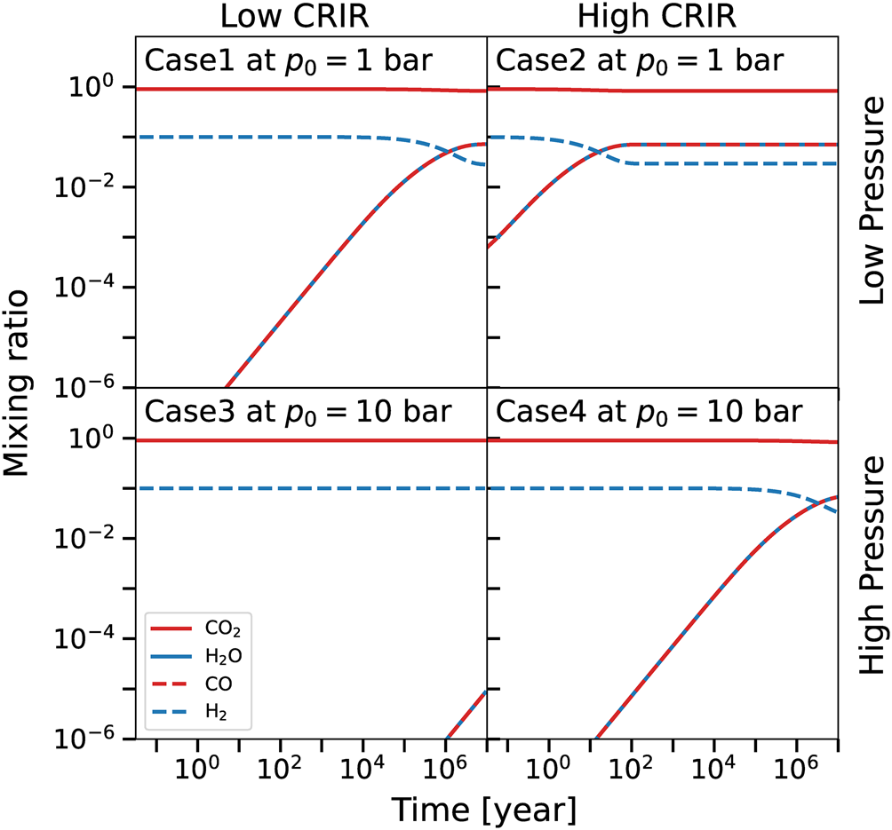
Fig. 6. Time evolution in the surface layer of the abundances of CO2 (solid red), H2O (solid blue), CO (dashed red) and H2 (dashed blue), for the different models. Molecular oxygen and ozone are not reported having mixing ratios well below the scale of the plot. Upper/lower row reports low-/high-pressure cases, while the first/second column shows low-/high-CRIR. For Case1 and Case2 the surface layer is p = 1 bar, while for Case3 and Case4 p = 10 bar, see Fig. 2.
In the surface layer (Fig. 6) CO and water are always coupled, and a clear molecular-hydrogen-to-water conversion is present, as well as the self-similarity of the four cases. The CO–water coupling is determined by the same reasons discussed in the vertical profile section, while the time-scale of the molecular-hydrogen-to-water conversion is a direct consequence of the amount of CRIR and the different densities (note that Case3 and Case4 have a ten times higher pressure). In fact, Case3, where the CRIR have the largest attenuation, presents the slowest chemical kinetics, that does not reach the equilibrium even after 107 years. Conversely, in the high-CRIR and low-density Case2, the CRIR determines the shortest time-scale of the molecular-hydrogen-to-water conversion, since CRIR is less attenuated. Analogously, Case1 and Case4 have a similar behaviour, since the CRIR has similar values closer to the surface (cf. Fig. 2).
These results show how the interplay between cosmic rays and the density structure of the moon determines the formation of water in the different layers and at different epoch (see Fig. 2). In each case the total amount of water formed is similar, but with different time-scales (see Fig. 3). Although cosmic rays are crucial in determining the total abundance of species and to shape the chemistry of the middle and upper layers, in the ground layer(s) the density profile of the atmosphere plays a key role. In particular, an high-pressure and high-CRIR environment (Case4) mimics the behaviour of a low-density and low-CRIR model (Case1), due to the similar cosmic rays attenuation (see e.g. Fig. 6). These results suggest that the role of the variation in the temperature vertical profile is less relevant when compared to the cosmic rays attenuation effect, except in the upper layers, where the temperature affects the amount of water formed. However, note that contribution of the upper layers to the total mass is less relevant when compared to the lower layers (see Fig. 3).
Discussion and conclusion
We modelled the time-dependent chemical evolution of the atmosphere of a 1 M$_\oplus$ exomoon orbiting around a 1 MJ FFP. Rather than the radiation of the hosting star, CRIR is the main driver of the chemical kinetics, and the main source of heating are the tidal forces exerted by the planet onto its moon. We determined the amount of water produced in the CO2-dominated atmosphere assuming an initial 10% of H2, and we measured the corresponding formation time-scale when changing the pressure at the base of the atmospheric vertical profile, the impinging CRIR, and the orbital parameters responsible for the tidal heating, namely semi-major axis and eccentricity.
Our findings suggest that a significant amount of water can be formed in the atmosphere of the exomoon and maintained in liquid form. In the low-pressure cases Case1 and Case2, i.e. the two models with the total atmospheric mass similar to Earth's, the amount of condensable water is of the order of 1017 kg at around 1 Myr and 100 years, respectively. For comparison, the total mass of Earth's oceans is ~ 1.4 × 10²¹ kg (Weast Reference Weast1979), and the amount of water vapour is ~ 1015 kg (Trenberth and Smith Reference Trenberth and Smith2005). The comet 67P/Churyumov-Gerasimenko has a total mass of ~ 1013 kg of which 10% water is a plausible estimate (Choukroun et al. Reference Choukroun, Altwegg and Kührt2020).
For the high-pressure model Case4 we obtain a water mass of 1.27 × 10¹⁸ kg at around 10 Myr. For comparison, on Venus, where the atmosphere is CO2-dominated and ~10 times denser than our high-pressure cases, the mixing ratio of water at the surface is 20 ppm (smaller than our findings in general, excluding Case3), while the total mass of water in the atmosphere is 4 × 10¹⁵ kg (Svedhem et al. Reference Svedhem, Titov, Taylor and Witasse2007). However, on Venus the temperature and the pressure measured at the surface do not allow the presence of liquid water (Way and Del Genio Reference Way and Del Genio2020). Mars also has a CO2-dominated atmosphere, but considerably less massive than the atmosphere of Venus and hence not capable of any efficient greenhouse effect and to retain liquid water. The estimated amount of water in the Martian atmosphere is ~2 × 10¹² kg (Jakosky et al. Reference Jakosky and Farmer1982).
Given the boundary conditions, our results allow us to classify this exomoon as a Class II environment (Lammer et al. Reference Lammer, Bredehöft and Coustenis2009), corresponding to bodies that allow life, but differ from a Class I habitat, i.e. an Earth-like water-rich world. It is worth noticing that when comparing our model to Earth, we are ignoring any external mechanism of water accretion (e.g. from asteroids, Jin and Bose Reference Jin and Bose2019)), and we compare a CRIR-dominated with a radiation-dominated atmosphere, the latter deeply affecting the atmospheric chemistry (see e.g. Hu et al. Reference Hu, Seager and Bains2012).
To maintain the temperature above the freezing point, the orbital parameters need to be constrained in time. As previously discussed, albeit surviving moons around ejected gas giants are expected to exist up to 0.1 au from the hosting planet, closer orbits ($\lesssim \!0.01$ au) are in general more probable (Rabago and Steffen Reference Rabago and Steffen2019). Figurefig1 shows that, given the same pressure conditions, for the same eccentricity value, smaller semi-major axis implies warmer environments. However, the eccentricity is expected to decrease with time, towards a more circular orbit (e → 0), that corresponds to a reduction of the surface temperature, with a subsequent water solidification. This mechanism can be prevented by resonances (Debes and Sigurdsson Reference Debes and Sigurdsson2007; Hong et al. Reference Hong, Raymond, Nicholson and Lunine2018) that are known to survive the ejection of the FFP from the hosting stellar system, allowing the stability of the orbital parameters over time, and hence the capability of the atmosphere to retain liquid water (Rabago and Steffen Reference Rabago and Steffen2019). A possible follow-up of our study consists of exploring the chemical evolution with the evolution of the orbital parameters.
The main conclusions of this study can be then summarized as follows:
• We found that an exomoon orbiting around an FFP provides an environment that might sustain liquid water onto its surface if the optical thickness of the atmosphere is relatively large and the orbital parameters produce enough tidal heating to increase the temperature over the melting point of water. These orbital parameters are in agreement with previous simulations (Debes and Sigurdsson, Reference Debes and Sigurdsson2007, Reference Debes and Sigurdsson2007, Hong et al., Reference Hong, Raymond, Nicholson and Lunine2018, Rabago and Steffen, Reference Rabago and Steffen2019) and within the explored eccentricities (between 10−3 and 0.5) and semi-major axis (between ~ 10−3 and ~ 10−2 au).
• Due to the absence of impinging radiation, the time-scale of water production is driven by the efficiency of cosmic rays in penetrating the atmosphere. Higher CRIRs reduce the water formation time-scale when compared to low-CRIR models, implying that they play a key role in the chemical evolution, by enhancing the chemical kinetics. However, due to the attenuation of cosmic rays, in the lower layers of the atmosphere, the water production is also affected by the density structure, that determines the integrated column density through the atmosphere. This causes an altitude-dependent abundance of water as well as of some of the other chemical species, as CO, H2 and O2.
• The temperature structure and its value at the surface are suitable for maintaining liquid water, but they play a marginal role in affecting the chemical evolution in the lower atmospheric layers (i.e. the main contributors to the total water mass) when compared to the effects of CRIR and their attenuation caused by the vertical density profile.
The presence of water on the surface of the exomoon, affected by the capability of the atmosphere to keep a temperature above the melting point, might favour the development of prebiotic chemistry (Kasting et al. Reference Kasting, Whitmire and Reynolds1993; Stevenson Reference Stevenson1999). According to Stevenson (Reference Stevenson1999), an FFP must have an effective temperature around 30 K to have liquid water on the surface. In our model the minimum effective temperature is ~97 K for a surface pressure of 10 bar, in a CO2-dominated atmosphere. The surface temperature is determined by the presence of greenhouse gases in the atmosphere (e.g. CO2) that control the heating produced by tidal forces. Under these conditions, if the orbital parameters are stable to guarantee a constant tidal heating, once water is formed, it remains liquid over the entire system evolution, and therefore providing favourable conditions for the emergence of life.
Acknowledgements
We thank the anonymous referees for improving the quality of this study. SB acknowledges support from the BASAL Centro de Astrofisica y Tecnologias Afines (CATA) AFB-17002. This study was funded by the DFG Research Unit FOR 2634/1 ER685/11-1. SOD has been founded by Sophia University Special Grant for Academic Research and JSPS KAKENHI Grant Numbers 17H06105, 20H01975 and 26108511. This research was supported by the Excellence Cluster ORIGINS, which is funded by the Deutsche Forschungsgemeinschaft (DFG, German Research Foundation) under Germany's Excellence Strategy – EXC-2094 – 390783311 (http://www.universe-cluster.de/).


