NOMENCLATURE
- A
cross-section area
- k
number of elements
- mi
local fuel mass fraction
- mmean
mean fuel mass fraction
- N
number of elements
- NI
non-uniformity index
- NIsup
supplementary non-uniformity index
- nair
air mole or mass fraction
- nfuel
fuel mole or mass fraction
- nmean
mean fuel mole fraction
 $n_{rms}^2$
variance of fuel mole fluctuations
- T
temperature
- $\Delta$T
linearised temperature increment
- dT
temperature increment
- U
unmixedness parameter or axial velocity component
- |U|
velocity magnitude
- UI
uniformity index
- X
perpendicular coordinate
- Y
vertical coordinate
- Z
longitudinal coordinate
- Φ
fuel/air equivalence ratio
- dΦ
fuel/air equivalence ratio increment
- $\Delta$Φ
difference between the maximum and minimum equivalence ratio or linearised Φ increment
- $\overline {\Delta\emptyset } $
averaged absolute fuel/air equivalence ratio deviation from the mean value


1.0 INTRODUCTION
For a fuel/air mixer design, it is of primary importance to keep the fuel distribution at the mixer exit as uniform as possible. It is well-known that NOx emission is closely related to the temperature and turbulence distributions inside the combustorReference Jiang and Campbell1, while the temperature field is mainly determined by the fuel distribution and airflow arrangementReference Lefebvre2. As pointed by Miller & BowmanReference Miller and Bowman3 and CorreaReference Correa4, the NOx formation is a notably nonlinear function of temperature and intimately associated with turbulence mixing process. The thermal NOx formation rate at temperature around 2200 K can be doubled due to a 90 K temperature increment. Therefore, to avoid high-temperature pockets in the combustor for NOx emission reduction, fuel-rich or high fuel/air equivalence ratio regions at the mixer exit should be avoided.
Fuel/air mixing uniformity is also required for many other combustor performance parameters, such as efficiency, safety, economy, etc. For example, to achieve high efficiency, nozzle guide vanes behind a gas turbine combustor are always exposed to high-temperature, high-pressure and high-dynamic load environmentsReference Saravanamuttoo, Rogers and Cohen5, causing the vanes to be one of the most failure-prone components in an engineReference Jiang, Han, Zhang, Wu, Clement and Patnaik6. It has been shown that to reduce the hot-streak effect from the combustor and extend the service life of turbine components, the temperature distribution at the combustor exit should be as uniform as possible, which is intimately correlated to the fuel/air mixing quality.
An adequate method to evaluate quantitatively the uniformity of fuel/air mixing is essential for research and development of advanced low-emission combustion systems. During the recent design of a propane/air mixer, it was noted that a suitable criterion to assess properly fuel/air mixing quality was not found in the open literature. Although papers reported the design or optimization of fuel/air mixers, such asReference Chandekar and Debnath7–Reference Danardono, Kim, Lee and Lee8, no quantitative uniformity values were given, rather only fuel fraction contour plots.
Currently, there are two criteria to evaluate fuel/air mixing quality. The first one is the unmixedness parameter for “goodness of mixing” introduced by DanckwertzReference Danckwertz9 as
 \begin{equation}U = \frac{{n_{rms}^2}}{{{n_{mean}}\;\left( {1 - \;{n_{mean}}} \right)}}\end{equation}
where  $n_{rms}^2$ is the variance of fuel mole fluctuations in time or space; and nmean stands for the mean fuel mole fraction. The parameter provides a statistical value of unmixedness “averaged” over a time interval or space. It has been successfully used to study the influence of temporal fuel mole fraction fluctuations on NOx emissions from lean premixed combustion by FricReference Fric10.
The second criterion is the uniformity index (UI), which is used by the internal engine communityReference Kim, Kim, Yoon and Sa11 and can be expressed as
 \begin{equation}UI=1 - \frac{1}{{2k}}\mathop \sum \limits_{i=1}^k \frac{{\sqrt {{{\left( {{m_i} - {m_{mean}}} \right)}^2}\;} }}{{{m_i}}}\end{equation}
where mi is the local fuel mass fraction, and mmean represents the mean fuel mass fraction. In Eq. (2), the unmixedness is represented by the second item on the right, which is also statistically “averaged.”
The advantages and shortcomings of the two criteria can be readily assessed from their definitions. The main advantages are that a statistically averaged assessment of fuel/air non-uniformity is provided over the cross-section, and they are valuable to study the effect of fuel fluctuations on combustion flow-field, such as NOx emission. The shortcomings of these definitions are that they are not directly correlated to the fuel/air mixture combustion property, and the peak unmixedness area is smeared by the averaging process.
Here a non-uniformity index, based on the fuel/air equivalence ratio distribution, is introduced as
 \begin{equation}NI = \frac{{{\emptyset _{max}}\; - \;{\emptyset _{min}}}}{{{\emptyset _{mean}}}} = \;\frac{{\Delta\emptyset }}{{{\emptyset _{mean}}}} = \frac{{{{\left( {{n_{fuel}}/{n_{air}}} \right)}_{max}} - \;{{\left( {{n_{fuel}}/{n_{air}}} \right)}_{min}}}}{{{{\left( {{n_{fuel}}/{n_{air}}} \right)}_{mean}}}}\end{equation}
where Φmax, Φmin and Φmean are the maximum, minimum and mean fuel/air equivalence ratios at a cross-section,  $\Delta$Φ represents the difference between the maximum and minimum equivalence ratio, and nfuel and nair stand for the mole or mass fraction of fuel and air, respectively. The NI accounts for the maximum variation of fuel/air equivalence ratio at the cross-section normalised by the mean equivalence ratio.
With this approach, the maximum temperature variation caused by the non-uniformity at the cross-section can be assessed. It is noted that, for combustion in air of methane, propane, and hydrogen, the flame temperature varies almost linearly with the equivalence ratio in a range of 0.55 – 0.75Reference Jadidi, Moghtadernejad and Dolatabadi12, and most combustion facilities or engines are operated within this range. Consequently, for a small number of  $\Delta$Φ, the temperature variation at the cross-section can be readily estimated by
 \begin{equation}\Delta T\; = \;\frac{{dT}}{{d\emptyset }}\;d\emptyset \approx \frac{{\Delta T}}{{\Delta\emptyset }}\;\Delta\emptyset = \;\frac{{\Delta T}}{{\Delta\emptyset }}\;{\emptyset _{mean}}\;NI\;\;\end{equation}
where  $\Delta$T is the estimated maximum temperature variation, dT and
  $\Delta$T stand for the temperature increment and linearised temperature increment, and dΦ and
  $\Delta$Φ represent the fuel/air equivalence ratio increment and linearised fuel/air equivalence ratio increment, respectively.
If the  $\Delta$Φ value is outside the linear approximation range,
  $\Delta$T can be obtained from the adiabatic flame temperature vs fuel/air equivalence ratio curve (T-Φ),
 \begin{equation}\Delta T \approx T\left( {{\emptyset _{max}}} \right) - T\left( {{\emptyset _{min}}} \right)\end{equation}
where T(Φ) is the mixture adiabatic temperature as a function of the fuel/air equivalence ratio. In Eq. (5), both Φmax and Φmin should be on the fuel lean or rich side; otherwise, Φ ≍ 1 should be considered.
The advantages of this alternative criterion are that the maximum variation of fuel/air mixing at the cross-section is captured, it is correlated to the mixture combustion property (temperature), and the maximum temperature variation caused by fuel/air non-uniformity can be estimated. This criterion is more stringent for fuel/air mixing quality control than the previous two criteria since the maximum non-uniformity is considered.
It is recognised that for all three criteria, for a given value of each criterion, the number of fuel/air distribution patterns is infinite. That is, the fuel/air distribution pattern is not uniquely defined by this value. Let us consider the mean fuel/air equivalence ratio at a cross-section A, expressed by Eq. (6).
 \begin{align}{\emptyset _{mean}} &= \mathop \smallint \nolimits_1^N \frac{{{\emptyset _i}dA}}{A} = \frac{{\mathop \smallint \nolimits_1^{{N_ + }} {\emptyset _ + }dA + \mathop \smallint \nolimits_1^{{N_ - }} {\emptyset _ - }dA}}{A} \nonumber\\ &= \frac{{\mathop \smallint \nolimits_1^{{N_ + }} \left( {{\emptyset _ + } - {\emptyset _{mean}} + {\emptyset _{mean}}} \right)dA + \mathop \smallint \nolimits_1^{{N_ - }} \left( {{\emptyset _ - } - {\emptyset _{mean}} + {\emptyset _{mean}}} \right)dA}}{A}\end{align}
where Φi, Φ+ and Φ− stand for the ith element, the element with equivalence ratio higher than the mean value, and the element with equivalence ratio less than the mean value; and N+ and N− represent the number elements for Φ+ and Φ−, respectively. From Eq. (6), the expression (7) can be obtained
 \begin{equation}\mathop \smallint \nolimits_1^{{N_ + }} \left( {{\emptyset _ + } - {\emptyset _{mean}}} \right)dA = \; - \mathop \smallint \nolimits_1^{{N_ - }} \left( {{\emptyset _ - } - {\emptyset _{mean}}} \right)dA\end{equation}
Equation (7) states that the integration of positive equivalence ratio deviations from the mean value over the cross-section is equal to that of negative deviations in terms of absolute values. This implies that the positive Φ deviation from the mean value averaged over the whole cross-section is equal to the absolute negative Φ deviation averaged over the cross-section. Moreover, if the Φ variation with temperature remains in linear relationship, the positive temperature deviation averaged over the cross-section is equal to the averaged absolute negative temperature deviation.
For the fuel/air mixing cases where the non-uniformity is considerably large, such as occurs when the fuel/air mixing length is limited or the fuel equivalence ratio varies substantially at the mixer exit, an additional statistical supplement criterion is required, which is introduced as
 \begin{equation}N{I_{sup}} = \frac{{\mathop \sum \nolimits_1^N \left| {{\emptyset _i} - {\emptyset _{mean}}} \right|/N}}{{{\emptyset _{mean}}}} = \frac{{\mathop \sum \nolimits_1^N \left| {\Delta{\emptyset _i}} \right|/N}}{{{\emptyset _{mean}}}} = \frac{{\overline {\Delta\emptyset } }}{{{\emptyset _{mean}}}}\end{equation}
where  $\Delta$Φi stands for the local fuel/air equivalence ratio deviation, and
  $\overline {\Delta\emptyset } $ is the statistically averaged absolute equivalence ratio deviation. Note that for the alternative criterion (Eq. (3)), the maximum variation of equivalence ratio at the cross-section is considered, while for the supplementary criterion (Eq. (8)), the averaged absolute equivalence deviation from the mean value is concerned.
Following the approach of Eqs. (4) and (5), a temperature deviation from the mean or designed value can be approximately estimated from one of the following two equations
 \begin{equation}\Delta T\; \approx \frac{{\Delta T}}{{\Delta\emptyset }}\;\overline {\Delta\emptyset } = \;\frac{{\Delta T}}{{\Delta\emptyset }}\;{\emptyset _{mean}}\;N{I_{sup}}\;\;\end{equation}
 \begin{equation}\Delta T \approx T\left( {{\emptyset _{mean}} + \overline {\Delta\emptyset } } \right) - T\left( {{\emptyset _{mean}}} \right)\end{equation}
Although the value obtained from Eq. (9) or Eq. (10) is not accurate as desired, it remains a good statistical assessment of non-uniformity and a “rough reference” of temperature deviation. In short, for the situations where the fuel/air distribution non-uniqueness issue should be considered, both the alternative and supplementary criteria should be used to check fuel/air mixing quality or setup targets for fuel/air mixer design.
Note that the fuel/air equivalence ratio becomes infinite at the locations where the air mole or mass fraction is zero, such as in the fuel inlet. To apply the proposed method, the local zero-air spots should be excluded from the domain or cross-section of analysis. In addition, to apply this method to EGR (exhaust gas recirculation) engines where the chemical composition in the combustion chamber is composed of fuel, air, and gas mixture from EGR, the unburned fuel and un-consumed air or corresponding chemical species from EGR should be included to compute the actual fuel/air (or combustion) equivalence ratio in the domain, and the relationship of T vs Φ should be re-generated by including the recirculated exhaust gas mixture.
In this paper, the application of this approach is demonstrated in a simple methane/air venturi mixer. In the following sections, the mixer geometry, computational domain and mesh, boundary conditions, numerical methods, mixer flow field, distributions of fuel/air equivalence ratio and corresponding temperature, local fuel mole fraction variance, and calculated values of fuel/air mixing quality from the three criteria and one supplementary criterion at typical cross-sections are presented and discussed. Finally, a few conclusions are highlighted.
2.0 NUMERICAL SIMULATION OF A SIMPLE VENTURI METHANE/AIR MIXER
2.1 Geometry, computational domain and mesh
The simple venturi mixer geometry is given in Fig. 1, which is based on a classic venturi designReference Fowles and Boyes13. Although its geometry is simple in comparison with fuel/air mixers used for industrial burners or gas turbine combustors, the criterion approach is the same. The venturi portion consists of a 254 mm long air-inlet section, 88.9 mm long throat section, and 254 mm long mixing section. The diameter is 102.4 mm for both air-inlet and mixing pipes, and 71.1 mm for the throat. The venturi converging and diverging angles are 10.5° and 12.5°, respectively, and the corresponding total length of the venturi portion is 770.1 mm. Four small fuel pipes arranged at 90 degrees are connected to the middle of the throat section, and they are 91.4 mm long with a diameter of 9.1 mm. The downstream extension portion is 762 mm long and has the same diameter as that of the venturi mixing section.

Figure 1. Geometry of the venturi methane/air mixer.
The computational domain and mesh of the venturi mixer is illustrated in Fig. 2, where the boundary mesh is indicated in white. Fine grids were laid in the venturi throat section, and medium-fine grids were generated in the upstream and downstream sections. Wall boundary meshes were generated, and the grid independence was checked. Eventually, the mesh with 326,000 cells was used in the simulation, and the y+ values at all wall boundaries were in the range of 30 – 200.

Figure 2. Computational domain and mesh.
2.2 Boundary conditions and numerical methods
The boundary conditions of the methane/air venturi mixer are listed in Table 1, and the corresponding overall fuel/air equivalence ratio is 0.6.
Table 1 Boundary conditions

The thermal properties of methane and air at 5 bar and 300 K were used in the simulation, and the mass diffusivity of methane in air, 2.1x10⁻⁵ m2/s, was obtained fromReference Matsunaga, Hori and Nagashima14.
The variation of methane/air adiabatic flame temperature with equivalence ratio is shown in Fig. 3. It was generated with Cantera and GRI-MECH 3.0 chemical kinetics at 5 bar pressure and 300 K initial temperature15.

Figure 3. Methane/air adiabatic flame temperature vs equivalence ratio.
The linear relationship between the flame temperature and equivalence ratio can be approximated in the range of 0.55 – 0.75 and 1.2 – 2.0 by the following two expressions:
 \begin{equation}\Delta T{\rm{\;}} \approx {\rm{\;}}1763.4{\rm{\;}} \times {\rm{\;}}{\emptyset _{mean}}{\rm{\;}}AL{\rm{\;}}\left( {or{\rm{\;}}A{L_{sup}}} \right){\rm{\;}}(\Phi = 0.55 - 0.75)\end{equation}
 \begin{equation}\Delta T{\rm{\;}} \approx {\rm{\;}} - 742.0{\rm{\;}} \times {\rm{\;}}{\emptyset _{mean}}{\rm{\;}}AL{\rm{\;}}\left( {A{L_{sup}}} \right){\rm{\;}}(\Phi = 1.2 - 2.0)\end{equation}
For the range Φ=0.1 – 2.0, the T-Φ relationship can be represented by two fourth-order polynomial curves, shown by the blue and orange dotted lines, for Φ=0.1 – 1.025 and 1.025 – 2.0 respectively.
 \begin{align}T(\Phi)\approx-1412.7\Phi^{4}+3045.5\Phi^{3}-2959.6\Phi^{2}+3306.8\Phi+272.55(\Phi=0.1-1.025)\end{align}
 \begin{align}T(\Phi)\approx-540.95\Phi^{4}+3391.9\Phi^{3}-7745.5\Phi^{2}+6886.9\Phi+292.18(\Phi=1.025-2.0)\end{align}
The methane/air mixing in the mixer was solved with ANSYS CFD Premium16. The realisable k-ε turbulence model and its settings were selected for this simulation, which were successfully applied to a model combustor fueled with gaseous propaneReference Jiang17, and a can-annular gas turbine combustor fired by liquid jet fuelReference Jiang, Han, Zhang, Wu, Clement and Patnaik6.
A segregated solver with a second-order-accuracy scheme was used to resolve the flow-field. At convergence, the scaled residuals were less than 3.5×10⁻⁶ for velocity components and scalar items, and less than 9.0×10⁻⁵ for turbulent variables. The monitored flow parameters remained unchanged for the first four digits, which ensured that the flow field reached steady condition.
3.0 RESULTS AND DISCUSSION
3.1 Flow field of fuel/air mixer
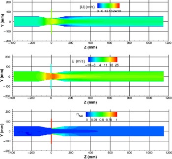
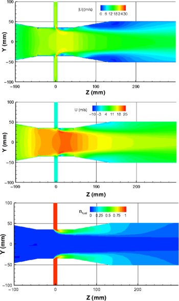
The mixer flow field is briefly mentioned here. Figure 4 presents the contour plots of velocity magnitude, axial velocity component and methane mole fraction along the longitudinal symmetric plane; whereas Fig. 5 provides magnified views of these parameters around the mixer throat section. Significant flow velocity variations occur across the venturi throat section. The high-velocity region exists in the throat section, and the maximum velocity magnitude reaches 30 m/s in the tiny downstream regions of the fuel entries. The maximum negative axial velocity component is about −10 m/s, which also occurs in the tiny downstream regions of the fuel entries. Fast fuel/air mixing is observed in the range of Z = 0 - 300 mm.

Figure 4. Contours of velocity magnitude, axial component and methane mole fraction at the longitudinal symmetric plane.

Figure 5. Magnified views of velocity magnitude, axial component and methane mole fraction around the mixer throat.
3.2 Equivalence ratio distribution and alternative criterion value
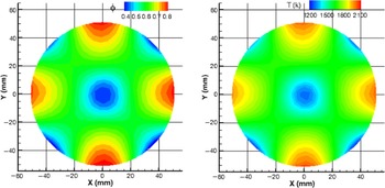
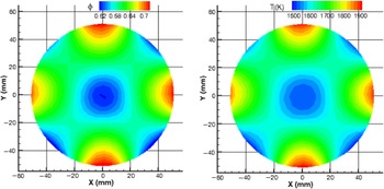
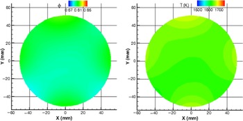
The contours of fuel/air equivalence ratio and corresponding temperature at five cross-sections — Z = 300, 400, 500, 800 and 1150 mm — are given in Figs 6–10, where the average Φ value is 0.6 for all these cross-sections. Due to the rapid decrease of Φ from section to section, the legend scales are different for sections Z = 300, 400 and 500 mm. In the last two figures, the same legend scales, Φ = 0.57 – 0.65 and T = 1500 – 1750 K, are used. Large variations of Φ and T are observed at Z = 300, 400 and 500 mm sections; whereas the Φ and T distributions at Z = 800 and 1150 mm cross-sections are much more uniform.

Figure 6. Φ and corresponding T distributions at Z = 300 mm.

Figure 7. Φ and corresponding T distributions at Z = 400 mm.

Figure 8. Φ and corresponding T distributions at Z = 500 mm.

Figure 9. Φ and corresponding T distributions at Z = 800 mm.

Figure 10. Φ and corresponding T distributions at Z = 1150 mm.
The non-uniformity index and supplementary criterion value, and corresponding equivalence ratio variation, averaged absolute equivalence ratio deviation from the mean value, maximum temperature variation and “reference” temperature at Z = 300, 400, 500, 800 and 1150 mm cross-sections are given in Table 2. Note that the averaged parameters in Table 2 are based on mass-weighted averaging. As expected, the two criteria values and corresponding temperatures monotonically decrease towards the mixer exit. The maximum temperature variations are much higher than the corresponding “reference” temperature deviations from the mean value. The reason is that for the former, the difference between the lowest and highest temperature across the cross-section is considered, whereas for the latter, a statistical average is concerned.
Table 2 NI, NIsup,  $\Delta$T and ∼
 $\Delta$T at Z = 300, 400, 500, 800 and 1150 mm cross-sections

More importantly, Table 2 indicates that for this demonstration case, if the mixture burns at the mixer exit, Z = 1150 mm section, the maximum temperature variation over the section can be ∼50 K due to the non-uniformity index of 4.59%. As an approximation, the maximum temperature deviation from the mean temperature could be considered as half of this value, i.e., ∼25K, which is good for many applications. Thus, the NI criterion can be used not only to check the fuel/air mixing, but also as a target for the mixer design.
If the situations where the maximum equivalence ratio or temperature variation is considerable large, such as at  $Z<1150$ mm sections, the supplementary criterion should also be used during mixer design optimisation. In this way, the maximum temperature variation across the cross-section is controlled by the NI criterion, and the supplemental criterion can be used to compare different design options. As a result, the best design from a thermal perspective can be identified.
3.3 Distributions of local fuel mole fraction variance and unmixedness parameter and uniformity index
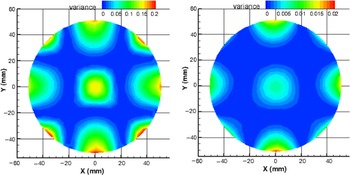
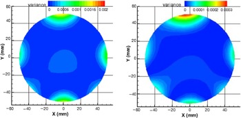
The fuel mole fraction variance,  $n_{rms}^2$ is used in the unmixedness parameter. The local fuel mole fraction variances (the square of fuel mole fraction deviation from the mean value) distributions, (ni – nmean)2, at Z = 300, 500, 800 and 1150 mm, are displayed in Figs 11–12. The parameter range varies dramatically from one section to another, and therefore the legend scale decreases sequentially about 10 times among these sections. In comparison of Figs 6 and 8 with Fig. 11, it is found that the four areas near the wall with high Φ values in Figs 6 and 8 also show high local variance in Fig. 11. However, the four areas near the wall and in the central region show low Φ values in Figs 6 and 8, but display high local variance in Fig. 11. This is because although Φ is low in these areas (in general, the Φ increment is negative), the local variance is always positive.

Figure 11. Local fuel mole fraction variance distribution at Z = 300 and 500 mm.

Figure 12. Local fuel mole fraction variance distributions at Z = 800 and 1150 mm.
The normalised absolute deviation of local fuel mass fraction from the mean value, |mi – mmean|/mi, is used in the uniformity index criterion. Similar trends as the fuel mole fraction variance are observed, although their contour plots are not presented here. This is because both the fuel mole fraction variance and the absolute fuel mass fraction deviation used by the two criteria are always positive.
Table 3 lists the computed values of the unmixedness parameter and uniformity index at Z = 300, 400, 500, 800 and 1150 mm sections, where the averaged parameters are based on mass-weighted averaging as in Table 2. For comparison, the corresponding NI and NIsup values are also listed in the table. As seen in the table, all four criteria provide good indications in terms of fuel/air mixing quality improvement. The further downstream the location, the better the fuel/air mixing. The values of the unmixedness parameter are pretty small, and it is about the order of 10E-5 at Z = 1150 mm, which is consistent with the observation in reference [10], and the parameter value varies sharply from one section to another. The values from other three criteria are in a range, 0.572% - 158%.
Table 3 U, UI, NI and NIsup at Z = 300, 400, 500, 800 and 1150 mm cross-sections

As mentioned earlier, since the U and UI criteria are not directly related to the fuel/air mixture combustion property, and do not catch the peaks of fuel/air mixing non-uniformity, the corresponding temperature variation and deviation are not available.
4.0 CONCLUSIONS
Fuel/air mixing uniformity is important to the development of advanced low-emission combustion systems. To provide a suitable criterion to estimate fuel/air mixing quality, a non-uniformity index, based on the fuel/air equivalence ratio distribution, is proposed, and successfully demonstrated in a simple methane/air venturi mixer.
The main advantages of the proposed criterion over the unmixedness parameter and uniformity index approaches are as follows: (1) it is correlated with the mixture combustion property, and (2) the maximum temperature variation caused by the fuel/air non-uniformity is captured. Therefore, it can be used not only as a criterion to check mixture uniformity, but also as a target for fuel/air mixer design with acceptable maximum temperature variation.
To avoid the effect of the fuel/air distribution non-uniqueness on fuel/air mixer design, for cases such as occur when the fuel/air mixing length is limited or the fuel equivalence ratio varies considerably at the mixer exit, the statistical supplement criterion discussed in this paper should be also included in design process in order to identify the best option.
It is author’s wish to raise the fuel/air mixing quality assessment issue to the combustion community, with the long-term goal of establishing an improved criterion for fuel/air mixer design and optimisation.
Acknowledgments
The author is grateful to Dr. Steve Zan for his valuable comments and suggestions during the preparation of this manuscript.