


1. Introduction
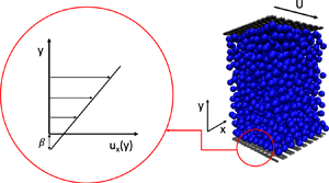
Accurate boundary conditions describing fluid behaviour at solid boundaries are essential to our ability to solve the Navier–Stokes equations or other models of hydrodynamic behaviour. The most prevalent such boundary conditions include the no-slip and slip conditions. In dilute gases, slip can be shown to arise due to the inhomogeneity introduced by the presence of the boundary (Hadjiconstantinou Reference Hadjiconstantinou2006; Sone Reference Sone2007). Asymptotic analysis of the Boltzmann equation shows that, to first order in the inhomogeneity, as quantified by the ratio of the mean free path to the system characteristic length scale (Hadjiconstantinou Reference Hadjiconstantinou2006; Sone Reference Sone2007), the slip velocity,  $u_s$ is described by the relation
 \begin{equation} u_s=\beta \frac{\partial u}{\partial \eta}, \end{equation}
where  $u$ denotes the flow velocity in the direction parallel to the boundary,
  $\eta$ denotes the boundary normal pointing into the fluid and
  $\beta$ denotes the slip length.
Relation (1.1) has also been empirically determined to describe slip in dense fluids and is known as the Navier slip condition (Navier Reference Navier1823). Although it can be derived from non-equilibrium thermodynamics considerations (Bedeaux, Albano & Mazur Reference Bedeaux, Albano and Mazur1976), this approach does not lead to a closed description in which the slip length can be predicted from knowledge of the system parameters. Progress towards the latter was made recently, when it was shown (Wang & Hadjiconstantinou Reference Wang and Hadjiconstantinou2019) that (1.1) can be obtained as the low-shear-rate limit of the nonlinear relation between the slip velocity and the shear rate (driving force), resulting from simple transition-state-theory arguments applied to the motion of fluid particles at the fluid–solid interface under the action of shear within the fluid and the potential imposed by the solid. Before this recent development, studies on the fundamentals of (1.1) mostly focused on determining the behaviour of the slip length, lumping any nonlinear relation between the slip velocity and the shear rate into that parameter. The most prevalent model of this type (Thompson & Troian Reference Thompson and Troian1997) assumes that the slip length is governed by some form of critical dynamics leading to a dependence on the shear rate,  $\dot {\gamma }$, of the form
 \begin{equation} \beta=\beta_0(1-\dot{\gamma}/\dot{\gamma}_c)^{-1/2}, \end{equation}
where  $\dot {\gamma }_c$ is a critical shear rate and
  $\beta _0$ the low-shear-rate slip length. The nature of the dynamics leading to this behaviour has yet to be identified. Taking a different approach, Lichter and collaborators (Lichter, Roxin & Mandre Reference Lichter, Roxin and Mandre2004; Martini et al. Reference Martini, Roxin, Snurr, Wang and Lichter2008) used molecular dynamics simulations to show that, for small to moderate driving forces, slip is a thermally activated process. As noted above, this observation was used by Wang & Hadjiconstantinou (Reference Wang and Hadjiconstantinou2019) to show that simple transition-state theory, of the type pioneered by Blake & Haynes (Reference Blake and Haynes1969) to model the motion of contact lines, can be used to capture many of the features of slip of a simple fluid at a solid boundary.
The most important drawback associated with simple transition-state theory is its use of ‘lumped parameters’, such as the jump-attempt frequency, which are difficult to calculate from first principles and rarely known a priori. In this paper, we formulate slip as forced Brownian motion in a periodic potential landscape and construct a detailed atomistic model that is amenable to accurate numerical solutions and allows analytical results in certain limits, thus providing a direct link between the microscopic physical picture and the observed macroscopic behaviour. Here, we note the approach by Barrat & Bocquet (Reference Barrat and Bocquet1999), who used Green–Kubo theory to relate the slip velocity to the dynamics of atoms subject to the corrugations of the potential landscape at the fluid–solid interface. Although at the same level of description, the Green–Kubo approach requires a number of approximations and is considerably less direct than the model proposed here. Despite these drawbacks, studies based on the Green–Kubo approach have led to a number of results (Barrat & Bocquet Reference Barrat and Bocquet1999; Priezjev & Troian Reference Priezjev and Troian2006; Priezjev Reference Priezjev2007a,Reference Priezjevb) that describe molecular simulation data well and are in qualitative agreement with our own results, as originally discussed by Wang & Hadjiconstantinou (Reference Wang and Hadjiconstantinou2019).
Following the discussion of some background material in § 2, the proposed model and its numerical solution is presented in § 3. Numerical solutions of the model are compared to molecular dynamics (MD) simulation results, both in house and from the study by Thompson & Troian (Reference Thompson and Troian1997), in § 4. The implications of the model for the slip length, as well as some analytical results, are discussed in § 5. We conclude with a discussion of our findings and possible future directions for research in § 6.
2. Background
We consider a dense fluid of viscosity  $\mu$ in contact with a stationary atomic wall. The fluid is subject to a uniform shear rate
  $\dot {\gamma }$. The equation describing motion parallel to the boundary for an atom in the first fluid layer can be written in the form
 \begin{equation} m\ddot{x}=-\eta_{FS}\dot{x}+\mu \dot{\gamma} \mathcal{A}+F_W+F_F, \end{equation}
where  $x$ denotes the atom location and overdots denote differentiation with respect to time,
  $m$ denotes the mass of the atom,
  $\eta _{FS}$ is the fluid–solid friction coefficient (Martini et al. Reference Martini, Roxin, Snurr, Wang and Lichter2008),
  $\mathcal {A}$ is the area per atom at the fluid–solid interface,
  $F_W$ denotes the force resulting from the periodic energetic barrier associated with the layered solid (period
  $\lambda$) and
  $F_F$ denotes the force exerted by all other fluid atoms on the atom of interest (beyond the shear force
  $\mu \dot {\gamma } \mathcal {A}$). Following common practice (Steele Reference Steele1973; Barrat & Bocquet Reference Barrat and Bocquet1999; Lichter et al. Reference Lichter, Roxin and Mandre2004; Martini et al. Reference Martini, Roxin, Snurr, Wang and Lichter2008), we take
  $F_W=-F_0\sin (2 {\rm \pi}x/\lambda )$, representing the largest term in a Fourier decomposition of the actual fluid–solid interaction potential; this is further discussed in § 6.
Lichter and collaborators (Lichter et al. Reference Lichter, Roxin and Mandre2004; Martini et al. Reference Martini, Roxin, Snurr, Wang and Lichter2008) argued about the need to include an atomistic-level description for  $F_F$, which, in its most typical form, namely,
  $F_F=\hat {k}\Delta x$, where
  $\Delta$ denotes the discrete Laplacian operator, transforms (2.1) into a Frenkel–Kontorova (FK) equation (Braun & Kivshar Reference Braun and Kivshar1998). They also recommended that the motion of fluid atoms normal to the boundary (in and out of the first fluid layer) be considered, making the governing equation a variable-density FK equation (vdFK), which could only be solved by simulation. Although some qualitative agreement between numerical solutions with in-house MD data was shown by Lichter et al. (Reference Lichter, Roxin and Mandre2004), a convincing rationale for the need for a model of this complexity was not established. In fact, our previous work (Wang & Hadjiconstantinou Reference Wang and Hadjiconstantinou2019), showed that the salient features of slip can be captured using a much simpler model based on simple transition-state theory of the type used to model the dynamics of contact lines with remarkable success (see, for example Blake et al. Reference Blake, Clarke, De Coninck and de Ruijter1997; de Ruijter, Blake & De Coninck Reference de Ruijter, Blake and De Coninck1999; De Coninck & Blake Reference De Coninck and Blake2008; Wang et al. Reference Wang, Damone, Benfenati, Poesio, Beretta and Hadjiconstantinou2019).
In this work we show that a model at the Langevin level of description can achieve a good balance between detailed modelling of the slip process at the atomistic scale and quantitative agreement with MD simulations. This level of description allows accurate solutions for the distribution function characterizing particle behaviour, thus avoiding all simplifications and assumptions associated with simple transition-state theory. Langevin equations of the type formulated and solved below have been studied in the past under the general topic of Brownian motion in periodic potentials, with applications to Josephson junctions and superionic conduction, among others (Risken Reference Risken1989).
3. Model formulation and solution
Within the Langevin formalism, as applied to the problem of interest here, the term  $F_F$ is modelled as a Wiener process with a variance related to the system temperature (Risken Reference Risken1989). With this assumption, after non-dimensionalization denoted by the subscript
  $n$, (2.1) can be written in the form
 \begin{equation} \ddot{x}_n+\zeta_n \dot{x}_n+d_n\sin x_n=F_n+\varGamma_n(t), \end{equation}
with
 \begin{equation} \langle \varGamma_n(t_n)\varGamma_n(t_n^{\prime})\rangle=2 \zeta_n\varTheta_n\Delta(t_n-t_n^{\prime}), \end{equation}
where  $\Delta(t)$ denotes the Dirac delta function,
  $x_n=2{\rm \pi} x/\lambda$,
  $t_n=2 {\rm \pi}t/\tau$,
  $\varTheta _n=\tau ^{2}k_BT/m \lambda ^{2}$,
  $\zeta _n=\tau \eta _{FS} /2 {\rm \pi}m$,
  $F_n= \tau ^{2} \mu \dot {\gamma } \mathcal {A}/ 2 {\rm \pi}m\lambda$ and
  $d_n=\tau ^{2} F_0/2{\rm \pi} m \lambda$. In the above,
  $k_B$ denotes Boltzmann's constant, while
  $\tau$ is a characteristic time scale of molecular magnitude that will be defined more precisely later. In the interest of simplicity, in what follows, the subscript
  $n$ will be omitted from non-dimensional quantities; instead, dimensional quantities will be denoted by a star.
Starting from (3.1) and using standard methods (Risken Reference Risken1989) one can arrive at the following Fokker–Planck equation
 \begin{equation} \frac{\partial \varPhi}{\partial t}=-\frac{\partial }{\partial x}(v \varPhi) +\frac{\partial }{\partial v}\left(\zeta v +d \sin x-F+\zeta\varTheta\frac{\partial}{\partial v}\right)\varPhi \end{equation}
governing the single-particle distribution function  $\varPhi =\varPhi (x,v,t)$, where
  $v=\dot {x}$. This equation describes a wide range of physical behaviour as the (effective) damping coefficient
  $\zeta$ varies. Although in the general case it needs to be solved numerically, analytical solutions are possible in the high-damping and the low-damping limit where simplifying assumptions can be made. It is thus important to establish the parameter regime in which Navier slip operates. As shown in the appendix, a first estimate based on typical magnitudes of physical quantities suggests that
  $\zeta \lesssim \delta \alpha /2{\rm \pi}$ with
  $\delta ,\alpha \sim O(1)$, which does not clearly fall under any of the two extreme limits of damping. As a result, we have proceeded to obtain solutions of (3.3) using the most general solution method (Risken Reference Risken1989) that is applicable to all values of
  $\zeta$. This procedure is described below.
3.1. Numerical solution of the Fokker–Planck equation
We are interested in steady (time-independent) solutions of (3.3) which are periodic in the interval  $0 \leqslant x \leqslant 2{\rm \pi}$ (
 $\varPhi (x+2{\rm \pi} )=\varPhi (x$)). Solution of this equation will allow the calculation of the drift velocity
 \begin{equation} \langle v\rangle=\int_{v=-\infty}^{\infty}\int_{x=0}^{2 {\rm \pi}} v \varPhi(x,v)\, {\textrm{d}\kern0.7pt x} \,\textrm{d}v \end{equation}
which corresponds to the macroscopic slip velocity (flow velocity of the layer of fluid atoms adjacent to the solid). The above assumes the normalization condition  $\int _{v=-\infty }^{\infty }\int _{x=0}^{2 {\rm \pi}} \varPhi (x,v) \,{\textrm {d}\kern0.06em x} \,\textrm {d}v=1$, which is automatically incorporated in the solution procedure outlined below.
The solution proceeds (Risken Reference Risken1989; Zheng & Hu Reference Zheng and Hu1995) using the expansion
 \begin{equation} \varPhi(x,v)=\varPsi_0(v)\sum_{j=0}^{\infty} C_j(x)\varPsi_j(v), \end{equation}
where
 \begin{equation} \varPsi_j(v)=\frac{H_j(v/\sqrt{2\varTheta})\exp(-v^{2}/4\varTheta)}{\sqrt{2^{j} j!\sqrt{2{\rm \pi}\varTheta}}} \end{equation}
and  $H_j(v)$ denotes the Hermite polynomial of order
  $j$ (Risken Reference Risken1989). Substituting the above expansion into (3.3) leads to the following infinite tridiagonal system of coupled ordinary differential equations for the coefficients
  $C_j(x)$
 \begin{equation} \left.\begin{gathered} \sqrt{1}\sqrt{\varTheta}C_1^{\prime}=0\\ \sqrt{1}\sqrt{\varTheta}C_0^{\prime}+1\zeta C_1+\sqrt{2}\sqrt{\varTheta}[C_2^{\prime}+C_2(d \sin x-F)/\varTheta]=0\\ \cdots=0\\ \sqrt{j}\sqrt{\varTheta}C_{j-1}^{\prime}+n\zeta C_j+\sqrt{j+1}\sqrt{\varTheta}[C_{j+1}^{\prime}+ C_{j+1}(d\sin x-F)/\varTheta]=0, \end{gathered}\right\} \end{equation}
where prime denotes differentiation with respect to  $x$ (
$x$ ( $C_j^{\prime }=\textrm {d}C_j/{\textrm {d}\kern0.06em x}$). The slip velocity can be shown to be given by
 \begin{equation} u_s=\langle v\rangle =2 {\rm \pi}C_1 \sqrt{\varTheta}, \end{equation}
where, according to the above hierarchy,  $C_1$ is a constant (
 $C_1\neq C_1(x$)) which depends only on the combinations
  $\zeta _\varTheta =\zeta /\sqrt {\varTheta }$,
  $F_\varTheta =F/\varTheta$ and
  $d_\varTheta =d/\varTheta$. This implies that the non-dimensional slip length
  $\beta =\langle v \rangle /F$ can be written in the form
 \begin{equation} \beta=\frac{1}{\zeta}\frac{2{\rm \pi} C_1\zeta_\varTheta}{F_\varTheta}=\frac{1}{\zeta}\varOmega(\zeta_{\varTheta},F_\varTheta,d_\varTheta), \end{equation}
where  $\varOmega$ is a function of
  $\zeta _\varTheta$,
  $F_\varTheta$ and
  $d_\varTheta$.
This infinite system of equations is solved by utilizing the periodicity of the solution, namely by expanding the coefficients  $C_j(x)$ into a truncated Fourier series
 \begin{equation} C_j(x)=\frac{1}{\sqrt{2{\rm \pi}}}\sum_{k=-Q}^{Q} (c_j)_k \,\textrm{e}^{\textrm{i}kx} \end{equation}
which, coupled to the continued fraction method (Risken Reference Risken1989), leads to a linear system of equations for determining the value of  $C_1$. The approximation in this numerical solution enters from the truncation of the infinite system of ordinary differential equations to a finite number (
 $J$) and the truncated Fourier series (3.10) utilizing
  $2Q+1$ terms. It can be shown (Risken Reference Risken1989) that truncation to
  $J=1$ corresponds to the limit
  $\zeta \rightarrow \infty$ (Smoluchowski equation); in other words, accurate solutions for the low-damping limit require a large
  $J$. Risken & Vollmer (Reference Risken and Vollmer1979) empirically found that
  $J=20/\zeta _\varTheta$ and
  $Q=12$ provides accurate solutions to at least 3 significant digits for
  $d_\varTheta \leqslant 4$. In this work we used
  $Q=25$ and
  $J=4000$, which can be verified to be consistent with or exceed (in terms of fidelity) the recommendations of Risken and Vollmer.
Figure 1 shows the behaviour of the slip length (times the friction coefficient) as a function of the driving force  $F_\varTheta$ for
  $d_\varTheta =2$ and four values of
  $\zeta _\varTheta$, namely 0.1, 0.5, 2 and 10. For a fixed
  $\zeta$, the observed behaviour is qualitatively similar to that observed by Lichter et al. (Reference Lichter, Roxin and Mandre2004) in their MD simulations and numerical solutions of the vdFK model: at small driving force, the existence of a region of linear response, which corresponds to a constant slip length, is evident. Analytical expressions for the slip length in the limit of small friction coefficient, as well as further discussion, can be found in § 5. Beyond the linear regime, the slip length increases rapidly, especially for small values of
  $\zeta _\varTheta$. Finally, at sufficiently high forcing, the response saturates to a constant slip length equal to
  $1/\zeta$. This result is in quantitative agreement with the observation of Lichter et al. (Reference Lichter, Roxin and Mandre2004), who first reported the saturation in the slip length for large forcing. It can be derived by noting that in the limit
  $F\rightarrow \infty$, provided a stationary state is reached (
 $\ddot {x}=0$), averaging equation (3.1) leads to
 \begin{equation} \lim_{F\rightarrow \infty}\frac{\langle v \rangle}{F}=\frac{1}{\zeta}. \end{equation}
Based on the non-dimensionalization of § 2, the dimensional value of the slip length is given by  $\beta ^{*}=\beta \mu ^{*} \tau ^{*} \mathcal {A}^{*}/2{\rm \pi} m^{*}$, which in the present case translates to
  $\lim _{\dot {\gamma ^{*}}\rightarrow \infty }\beta ^{*}=\mu ^{*} \mathcal {A}^{*}/\eta _{FS}^{*}$. Here, we note that our present discussion assumes that
  $\mu ^{*}$ remains constant at these very high shear rates, which is not always the case (Heyes Reference Heyes1985). If high shear rates are of interest, this phenomenon can be taken into account by using
  $\mu ^{*}=\mu ^{*}(\dot {\gamma }^{*})$ in (2.1).

Figure 1. Slip length times the friction coefficient,  $\beta \zeta$, as a function of
  $F_\varTheta$ for
  $d_\varTheta =2$ and
  $\zeta _\varTheta =0.1$ (blue), 0.5 (red) and 2 (yellow) 10 (purple). The linear response (constant slip length) is evident for small forcing. At high forcing the response saturates to the prediction of (3.11).
4. Comparison with molecular dynamics simulations
In this section we compare solutions of the model proposed here with MD simulation results available in the literature. The data used here involve simple Lennard–Jones (LJ) fluids and are in the form of the (non-dimensional) slip velocity  $u_s=u_s^{*}\tau _{LJ}^{*}/\sigma ^{*}$ as a function of the (non-dimensional) shear rate
  $\dot {\gamma }={\dot {\gamma }}^{*} \tau _{LJ}^{*}$, where
  $\tau ^{*}_{LJ}=\sqrt {m^{*}{\sigma ^{*}}^{2}/\varepsilon ^{*}}$ denotes the LJ characteristic time,
  $\sigma ^{*}$ the associated LJ potential characteristic distance and
  $\varepsilon ^{*}$ the LJ potential well depth; all of the above parameters refer to the fluid–fluid LJ interaction.
To facilitate comparison in these units, we take  $\lambda ^{*}=\delta \sigma ^{*}$ and
  $\tau ^{*}=\delta \tau _{LJ}^{*}$ with
  $\delta$ denoting a constant of order one; this leads to
  $\zeta =\delta \tau _{LJ}^{*}\eta _{FS}^{*}/2{\rm \pi} m^{*}$,
  $d=F_0^{*}\lambda ^{*}/\varepsilon ^{*}$, which represents the barrier height normalized by
  $\varepsilon ^{*}$, such that
  $d_\varTheta$ represents the barrier height normalized by
  $(k_BT)^{*}$ and
  $F=f \cdot (\dot {\gamma }^{*}\tau _{LJ}^{*})$, where
  $f=(\delta \alpha /2{\rm \pi} )\cdot (\mathcal {A}^{*}/{\sigma ^{*}}^{2})$; the latter is obtained by noting that for a LJ fluid
  $\mu ^{*}= \alpha \varepsilon ^{*} \tau _{LJ}^{*} {\sigma ^{*}}^{-3}$, where
  $\alpha \sim O(1)$ (for example,
  $\alpha =2$ for the data in Thompson & Troian Reference Thompson and Troian1997).
Given that the temperature of the simulations is known in each case, our comparison uses a nonlinear fit to determine the values for the parameters  $\zeta$,
  $d$ and the prefactor
  $f$. To reduce computational cost and assist with convergence, all parameters were constrained to be positive; moreover,
  $f$ was constrained to be in the range
  $0.2 \leqslant f \leqslant 4$. The latter follows from our estimate that
  $f$ is expected to be of order unity detailed above.
Figures 2 and 3 show a comparison with MD data from Thompson & Troian (Reference Thompson and Troian1997), performed at  $\varTheta =1.1$ and fluid density
  $\rho =0.81$ (in LJ units). The figures show the slip velocity as a function of the shear rate for different values of the fluid–solid interaction parameter
  $\varepsilon _{FS}$ for two different cases of fluid–solid interactions and wall structures. The agreement between MD simulation and theory is generally very good. Particularly gratifying is the consistency and rational trends in the model parameters returned by the fitting routine, including their agreement with our preliminary estimates. For example, for each wall structure, a monotonically increasing value of
  $\varepsilon _{FS}$ (at fixed
  $\varepsilon ^{*}$) leads to a monotonically increasing value of the barrier height
  $d$. We also observe that the value of the barrier height has a strong effect on the resulting slip. This is as expected in thermally activated motion; it will be further discussed in the next section where some analytical results are presented.

Figure 2. Comparison between MD simulation data from Thompson & Troian (Reference Thompson and Troian1997) and the proposed model, for two fluid–solid interaction parameter values  $\varepsilon _{FS}=0.6,0.1$ (a,b), at fixed solid density
  $\rho _S=1$, fluid–solid length scale parameter
  $\sigma _{FS}=1$, fluid density
  $\rho =0.81$ and temperature
  $\varTheta =1.1$. Best fit parameters:
  $\zeta =0.088, d=2.07, f=0.6$ (a);
  $\zeta =0.056, d=1.51, f=0.6$ (b).

Figure 3. Comparison between MD simulation data from Thompson & Troian (Reference Thompson and Troian1997) (circles) and the proposed model (solid lines), for three fluid–solid interaction parameter values  $\varepsilon _{FS}=0.6,0.4,0.2$ (a–c), at fixed solid density
  $\rho _S=4$, fluid–solid characteristic distance
  $\sigma _{FS}=0.75$, fluid density
  $\rho =0.81$ and temperature
  $\varTheta =1.1$. Best fit parameters:
  $\zeta =0.02, d=1.18, f=0.47$ (a);
  $\zeta =0.02, d=1.11, f=0.72$ (b);
  $\zeta =0.02, d=0.74, f=1.02$ (c).
Figure 4 shows a comparison with two sets of data from Wang & Hadjiconstantinou (Reference Wang and Hadjiconstantinou2019) with  $\varTheta =5$ and corresponding to two sets of fluid densities, namely
  $\rho =0.6$ and
  $\rho =1.0$. The agreement between the MD data and the model is excellent and leads to physically reasonable parameter values that are consistent in overall magnitude with those found to fit the MD results of Thompson and Troian in figures 2 and 3. The non-dimensional friction coefficient is much smaller than unity, in agreement with our findings so far. Given that the only difference between the two cases shown in this figure is the fluid density, we would expect the barrier height to be approximately the same, while
  $f$ (proportional to the area per particle) to be higher in the lower-density case (Wang & Hadjiconstantinou Reference Wang and Hadjiconstantinou2017 have shown that the density of the fluid at the fluid–solid layer is proportional to the bulk fluid density). These expectations are reflected in the actual parameter values with remarkable accuracy.

Figure 4. Comparison between MD simulation data from Wang & Hadjiconstantinou (Reference Wang and Hadjiconstantinou2019) (circles) and the proposed model (solid lines), at temperature  $\varTheta =5$ and two fluid densities:
  $\rho =0.6$ (a) and
  $\rho =1.0$ (b). Best fit parameters:
  $\zeta =0.016, d=9.7, f=2.3$ (a), and
  $\zeta =0.013, d=9.7, f=1.7$ (b).
5. Slip length
Having established that Navier slip operates in the low- $\zeta$ regime, we revisit the governing equation (3.3) in this limit for which Risken and Vollmer have developed an asymptotic solution (Risken Reference Risken1989). Up to and including terms of order
  $\sqrt {\zeta _\varTheta }$, the slip velocity can be written in the form
 \begin{equation} \langle v\rangle=\frac{Z_3}{Z_0+Z_1}+\sqrt{\zeta_\varTheta}\frac{\sqrt{2}\chi}{\sqrt{s(d)\sqrt{\varTheta}}}\left(\frac{Z_4}{Z_0+Z_1}-\frac{Z_2Z_3}{(Z_0+Z_1)^{2}}\right)\hat{F} \end{equation}
where  $\hat {F}=F/\zeta$,
  $\chi =0.855$ and
 \begin{equation} \left.\begin{gathered} Z_0=\sqrt{\frac{{\rm \pi}\varTheta}{2}}I_0\left(d_\varTheta\right),\quad Z_1=\int_d^{\infty} s'(E)\exp\left(-\frac{E}{\varTheta}\right)\left[\cosh\left(\frac{\hat{F}g(E)}{\varTheta}\right)-1\right]\textrm{d}E\\ Z_2=\int_d^{\infty} s'(E)\exp\left(-\frac{E}{\varTheta}\right)\sinh\left(\frac{\hat{F}g(E)}{\varTheta}\right)\textrm{d}E,\\ Z_3=\int_d^{\infty} \exp\left(-\frac{E}{\varTheta}\right) \sinh \left(\frac{\hat{F} g(E)}{\varTheta}\right) \textrm{d}E\\ Z_4=\int_d^{\infty} \exp\left(-\frac{E}{\varTheta}\right) \cosh \left(\frac{\hat{F} g(E)}{\varTheta}\right) \textrm{d}E. \end{gathered}\right\} \end{equation}
In the above,  $I_0(x)$ is the modified Bessel function of order zero and
 \begin{equation} \left.\begin{gathered} g(E)=\int_d^{\infty} \frac{\textrm{d}E}{s(E)},\\ s(E)=\frac{2\sqrt{2}}{\rm \pi}\sqrt{E+d}\,{\textrm{E}}\left(\frac{2d}{d+E}\right),\\ s'(E)=\frac{\textrm{d}s}{\textrm{d}E}=\frac{\sqrt{2}}{{\rm \pi}\sqrt{E+d}} \,\mathrm{K} \left(\frac{2d}{d+E}\right), \end{gathered}\right\} \end{equation}
where  $\mathrm {K}(x)$ and
  $\mathrm {E}(x)$ denote the complete elliptic integrals of the first and second kind, respectively (Risken Reference Risken1989).
This solution is useful as a closed form alternative to the numerical solutions of § 3.1. As figure 5 shows, at the values of  $\zeta$ found to describe the MD data, it captures the reference numerical solution very well. One area where the analytical solution is particularly useful is the linear regime (
 $\hat {F}\ll 1$) in which it can be used to provide the following explicit result for the slip length
 \begin{align} \beta&=\frac{\langle v\rangle}{F} =\frac{1}{\zeta I_0(d_\varTheta)}\left(\sqrt{\frac{2}{{\rm \pi} \varTheta}}\int_d^{\infty} \frac{\exp\left(-E/\varTheta\right)}{s(E)}\textrm{d}E+ \chi\frac{\sqrt{\zeta_\varTheta} \exp\left(-d_\varTheta\right)}{\sqrt[4]{d_\varTheta}}\right)\nonumber\\ &=\frac{1}{\zeta I_0(d_\varTheta)}\left(\sqrt{\frac{2}{\rm \pi}}\int_{d_\varTheta}^{\infty} \frac{\exp\left(-\ell\right)}{w(\ell)}\textrm{d}\ell+\chi\frac{ \sqrt{\zeta_\varTheta}\exp \left(-d_\varTheta\right)}{\sqrt[4]{d_\varTheta}}\right),\quad \mathrm{for} \ \hat{F}\ll 1, \, \zeta_\varTheta\ll 1, \end{align}
where  $w(\ell )=2\sqrt {2}\sqrt {\ell +d_\varTheta }\,\mathrm {E}[2d_\varTheta /(d_\varTheta +\ell )]/{\rm \pi}$. Unfortunately, the presence of the elliptic integral in the definition of
  $w(\ell )$ prevents a full analytic result, except in the limit
  $d_\varTheta \rightarrow \infty$ where
  $I_0(d_\varTheta )\approx \exp (d_\varTheta )/\sqrt {2 {\rm \pi}d_\varTheta }$,
  $\int _{d_\varTheta }^{\infty } \exp (-\ell )/w(\ell )\,\textrm {d}\ell \approx \exp (-d_\varTheta )/w(d_\varTheta )$, thereby simplifying (5.4) further to
 \begin{equation} \beta=\left(\frac{\rm \pi}{2}+\chi \sqrt{2{\rm \pi}\zeta_\varTheta\sqrt{d_\varTheta}}\right) \zeta^{-1}\exp\left(-2d_\varTheta\right), \quad \mathrm{for}\ \hat{F}\ll 1, \ \zeta_\varTheta\ll 1,\, d_\varTheta \rightarrow \infty . \end{equation}
This result, although strictly asymptotic, displays more clearly the (decaying) exponential dependence of slip on the normalized barrier height ( $d_\varTheta$) that was also prominent in the simpler transition-state-theory-based model of Wang & Hadjiconstantinou (Reference Wang and Hadjiconstantinou2019).

Figure 5. Comparison between numerical solution (red) and analytical solution (5.1) (blue) for  $\zeta =0.02, d=1.18$ and
  $f=0.47$. The MD data from Thompson & Troian (Reference Thompson and Troian1997), for which these parameters were determined to provide the best fit (figure 3a), are also shown.
6. Discussion
We have developed and validated an atomistic model of the Navier slip condition. Our validation was focused on molecular simulations, for which atomistic-level details and associated parameter values are available. We hope to extend this work to more complex fluids, for which experimental data are more readily available, soon. The agreement found with a variety of MD simulation results using reasonable and consistent values of the model parameters, as well as the model's ability to capture the salient features of the slip phenomenon is very encouraging and suggests that fluid slip can be accurately described by a detailed molecular model of moderate complexity.
As in our previous work (Wang & Hadjiconstantinou Reference Wang and Hadjiconstantinou2019), we have focused on the low-forcing regime (low shear rates) which corresponds to typical shear rates of practical interest. Although high shear response may be a useful test for a proposed theory (e.g. whether it predicts the slip length plateau observed by Lichter et al. Reference Lichter, Roxin and Mandre2004), the high-shear-rate regime ( $\hat {F}\gg 1$) corresponds to physical shear rates that exceed
  $10^{8}\ \mathrm {s}^{-1}$ which are for all practical purposes only of academic interest.
It is notable that the MD results used here, modelling typical interfaces between a simple mildly hydrophilic fluid and a molecular solid, are best described by very low values of the (non-dimensional) friction coefficient  $\zeta$. From a qualitative point of view, the low values of
  $\zeta$ found to fit the MD data reflect the steep rise in slip exhibited by the data past the linear response region that cannot be captured by solutions with high
  $\zeta$ (see figure 1 for a comparison). Although within the bounds imposed by physical arguments and magnitudes of known physical quantities, the low values of
  $\zeta$ found here are in contrast to typical assumptions made in the literature in the course of modelling thermally activated atomic motion at the fluid–solid interface, such as the use of theoretical tools which assume overdamped physics. A more thorough investigation of this aspect should be undertaken in the future.
The present model can be improved in a number of ways, starting, perhaps, from a more accurate representation of the fluid–solid interaction potential. Assuming a simple sinusoidal form is very common in the literature and justified as the leading term in a Fourier expansion of the true (periodic) potential (Barrat & Bocquet Reference Barrat and Bocquet1999; Martini et al. Reference Martini, Roxin, Snurr, Wang and Lichter2008), even though this is not always a good representation of the actual potential field experienced by the fluid atoms at the fluid–solid interface. The methodology presented here is in no way limited to this potential form and can be easily extended to other periodic potentials, including the actual fluid–solid interaction potential, especially if numerical solutions are sufficient. We believe that a higher fidelity representation of this potential field, and a model for predicting the friction coefficient from knowledge of the fluid–wall interaction as well as fluid and wall properties, are the two final ingredients needed for predicting slip from first principles (atomistic-level description) using this approach.
Adding explicit interactions between fluid particles (e.g. in the spirit of the FK model discussed briefly in § 2) is possible within the Langevin formalism at the cost of increased dimensionality of the distribution function and the governing Fokker–Planck equation, which resides in the phase space of the positions and velocities of all particles involved. Although problems involving two interacting particles have been treated in the literature (Risken Reference Risken1989), it is clear that a formulation including more than one particle, so that particle interactions can be taken into account, will be significantly harder to treat in general and may only be amenable to numerical solutions.
Acknowledgements
The author would like to thank Dr G. Wang for many useful discussions and for providing the MD simulation data used for validation in § 4.
Declaration of interests
The author reports no conflict of interest.
Appendix
To estimate the magnitude of  $\zeta =\delta \tau _{LJ}^{*} \eta _{FS}^{*} /2 {\rm \pi}m^{*}$ we start with the observation by Martini et al. (Reference Martini, Roxin, Snurr, Wang and Lichter2008) that
  $\eta _{FS}^{*}\lesssim \eta _{LL}^{*}$ and usually
  $\eta _{FS}^{*}\ll \eta _{LL}^{*}$, where
  $\eta _{LL}^{*}=\mu ^{*} \mathcal { A}^{*}/a^{*}$, and
  $a^{*}$ is the fluid–fluid atomic spacing normal to the fluid–solid interface. Using
  $\eta _{FS}^{*}\approx \eta _{LL}^{*}$ as an upper bound and the observation that the viscosity of a simple LJ fluid is given by
  $\mu ^{*} = \alpha \varepsilon ^{*} \tau _{LJ}^{*} {\sigma ^{*}}^{-3}$ with
  $\alpha \sim O(1)$ and assuming
  $\mathcal { A}^{*}\sim {\sigma ^{*}}^{2}$ and
  $a^{*}\sim \sigma ^{*}$ (Wang & Hadjiconstantinou Reference Wang and Hadjiconstantinou2015, Reference Wang and Hadjiconstantinou2017), we obtain
  $\zeta \approx \delta \alpha /2{\rm \pi}$. We thus expect
  $\zeta \lesssim \delta \alpha /2{\rm \pi}$.


