INTRODUCTION
In recent years, skates have received increased attention in light of population declines and local extirpations of once-common species (Brander, Reference Brander1981; Dulvy et al., Reference Dulvy, Metcalfe, Glanville, Pawson and Reynolds2000). While considerable research effort has been directed at commercially important, shelf-dwelling species, much less effort has been expended upon deep-sea skates. Deep-water species of some groups have been shown to attain greater maximum ages than their shallow-dwelling counterparts, which translates to lower productivity and hence greater susceptibility to overfishing (Cailliet et al., Reference Cailliet, Andrews, Burton, Watters, Kline and Ferry-Graham2001; García et al., Reference García, Lucifora and Myers2008). In combination with documented declines in skate stocks in several regions, the current trend of fisheries' expansion into deeper waters (Koslow et al., Reference Koslow, Boehlert, Gordon, Haedrich, Lorance and Parin2000; Haedrich et al., Reference Haedrich, Merrett and O'Dea2001; Roberts, Reference Roberts2002; Morato et al., Reference Morato, Watson, Pitcher and Pauly2006) underscores the need to direct research effort towards the collection of basic life history information for poorly known, deep-dwelling members of skate assemblages.
Directed skate fisheries have developed in Alaskan waters in the past decade (Gburski et al., Reference Gburski, Gaichas and Kimura2007; Kenneth J. Goldman, Alaska Department of Fish & Game, personal communication), but the species-specific catch and life history data required to inform management are sparse. Until recently, skates in the eastern Bering Sea (EBS) were managed as a complex of ‘other species’ comprised several biologically discrete taxonomic groups, including sharks, sculpins, squid and octopus (Ebert et al., Reference Ebert, Maurer, Ainsley, Barnett and Cailliet2009). Beginning in 2011, skates were removed from the ‘other species’ category and are currently managed as a separate aggregate complex (Ormseth et al., Reference Ormseth, Matta, amd Hoff, Aydin, Clausen, Conners, Conrath, Dalton, DiCosimo, Echave, Goldman, Hanselman, Heifetz, Hoff, Honkalehto, Ianelli, Kotwicki, Lauth, Lowe, Lunsford, McKelvey, Matta, Nichol, Ormseth, Rodgveller, Rooper, Spencer, Spital, Spies, Stockhausen, TenBrink, Thompson, Tribuzio, Wilderbuer and Wilkins2010). Though this is an improvement over previous practices, results of studies conducted to date suggest that Alaskan skate species vary widely in maximum ages and ages-at-maturity, indicating high potential for shifts in assemblage structure in response to fishing pressure (McFarlane & King, Reference McFarlane and King2006; Ebert et al., Reference Ebert, Smith, Haas, Ainsley and Cailliet2007, Reference Ebert, Smith and Cailliet2008a, Reference Ebert, Maurer, Ainsley, Barnett and Cailliet2009; Gburski et al., Reference Gburski, Gaichas and Kimura2007; Matta & Gunderson, Reference Matta and Gunderson2007). Life history parameter estimates are available for nine of the fifteen known members of the Alaskan skate assemblage (McFarlane & King, Reference McFarlane and King2006; Ebert et al., Reference Ebert, Smith, Haas, Ainsley and Cailliet2007, Reference Ebert, Smith and Cailliet2008a, Reference Ebert, Maurer, Ainsley, Barnett and Cailliet2009; Gburski et al., Reference Gburski, Gaichas and Kimura2007; Matta & Gunderson, Reference Matta and Gunderson2007) but have yet to be produced for the deepest-dwelling species.
The roughtail skate, Bathyraja trachura, occurs in the EBS along the deep shelf and upper continental slope at depths of up to 2550 m (Ebert, Reference Ebert2003). The species has a relatively large geographical distribution in the eastern North Pacific (from northern Baja California to the Bering Sea) and is taken as by-catch in groundfish fisheries throughout its range, yet little information regarding the species is available in the literature. The only published age and growth study to date provided a maximum age estimate of 20 yr for specimens collected off the western coast of the continental USA (Davis et al., Reference Davis, Cailliet and Ebert2007). Reproductive data are also limited (Ebert, Reference Ebert2005). While the estimates currently available do provide a rough estimate of the relative productivity of the species, its large range of distribution indicates a high probability of geographical variation in life history parameters (Lombardi-Carlson et al., Reference Lombardi-Carlson, Cortés, Parsons and Manire2003; Frisk & Miller, Reference Frisk and Miller2006; Licandeo & Cerna, Reference Licandeo and Cerna2007; McPhie & Campana, Reference McPhie and Campana2009). Therefore, age estimates for B. trachura from the EBS are required to reliably assess the species' potential response to exploitation at the northern extent of its range.
This study addresses a gap in knowledge about the Alaskan skate assemblage by providing life history parameter estimates for B. trachura. Specifically, the objectives of this study were to determine the age and growth characteristics and estimate the size- and age-at-maturity of the species in the EBS. Results are compared with those previously reported for the species near the southern end of its range from the California Current (CC) ecosystem. Potential management implications are also discussed.
MATERIALS AND METHODS
Field sampling
Bathyraja trachura specimens were collected during fishery-independent surveys conducted in the EBS between June and August 2004 as part of the biannual National Marine Fisheries Service, Alaska Fisheries Science Center's (NMFS-AFSC) Eastern Bering Sea Continental Slope survey. The survey covered the EBS from an area north-west of Unalaska Island (55o95′N 168o92′W) to the Navarin Canyon (60o16′N 179o68′W) near the US–Russian border. Specimens were collected during 30 min bottom trawls (poly Nor'Eastern high-opening trawl equipped with mud-sweep roller gear and 127 mm stretched-mesh netting with a 32 mm mesh codend liner; Hoff & Britt, Reference Hoff and Britt2005) at depths of 624–1138 m. Trawl location was determined using a random stratified sampling design of the area with 83 pre-determined bottom trawl stations (Hoff & Britt, Reference Hoff and Britt2005). Location, depth of capture, and temperature were recorded for each haul. One additional sample was obtained from the same area during October 2007 by Jerry Hoff (Fishery Biologist, NMFS-AFSC).
Morphometric measurements taken at the time of collection included total length (TL, measured from the tip of the snout to the tip of the tail), disc width (DW), and total weight (W) when possible. All lengths and widths were recorded to the nearest mm. Total weights were recorded to the nearest 0.01 kg. For ageing, a minimum of ten vertebral centra was excised from a region posterior to the cranium between the 5th and 20th vertebrae and frozen at –20 to –23oC for future processing; vertebral centra were determined to be the most appropriate ageing structure for the species by using the methods of Davis et al. (Reference Davis, Cailliet and Ebert2007).
The TL of four skates could not be directly obtained due to tail damage. To estimate TL for those four specimens, a length conversion equation based on observed DW and TL values was derived. Initial scatterplots of TL and DW indicated a linear relationship. Since skates are sexually dimorphic (Ebert et al., Reference Ebert, Compagno and Cowley2008b; Orlov et al., Reference Orlov, Cotton and Shevernitsky2010), this relationship may differ between sexes. Therefore, a linear regression model was applied, with TL as the response variable, DW as a linear explanatory variable and sex as a factor. An interaction term between DW and sex was also included to determine whether the slope of this relationship differed between sexes. All analyses were conducted in R (R Core Team, 2012).
Analysis of residuals from the initial regression indicated that variance increased with DW, violating the assumption of homogeneity. Therefore, generalized least squares (GLS) estimation in the R package ‘nlme’ (Pinheiro et al., Reference Pinheiro, Bates, DebRoy and Sarkar2012) was used to allow for heterogeneity (Zuur et al., Reference Zuur, Ieno, Walker, Saveliev and Smith2009). The optimal regression model was identified from all possible model subsets as the model containing only significant terms (P < 0.05) with the smallest second-order Akaike information criterion value (AICc; Akaike, Reference Akaike, Petrov and Csaki1973; Burnham & Anderson, Reference Burnham and Anderson2002). The AICc difference (Δi) of each model was calculated based on the lowest observed AICc value (AICc,min) as
Models with Δi < 2 were considered indistinguishable (Burnham & Anderson, Reference Burnham and Anderson2002).
Vertebral preparation and age determination
Vertebral centra were collected from 154 B. trachura (94 males, 59 females, and one of unknown sex). Histological preparation of vertebrae followed Natanson et al. (Reference Natanson, Sulikowski, Kneebone and Tsang2007). Frozen vertebrae were thawed, cleaned of excess tissue with a scalpel, separated into individual centra, and fixed in 70% ethanol for a period of at least one month. Samples were then grouped by size and decalcified by immersion in RDO® rapid decalcifying agent. Decalcification was considered complete when a scalpel blade could pass easily through the centrum with no remaining evidence of calcification in the centre. Decalcification times ranged from 47 to 185 min depending on centrum size. Following decalcification, centra were rinsed with flowing water for one hour and stored in 70% ethanol until processing. Decalcified vertebrae were embedded in paraffin wax following a nine-step dehydration process. Embedded centra were sectioned to a thickness of 80–100 μm with a sledge microtome. Sections were stained with Harris haematoxylin and adhered to microscope slides (see Natanson et al., Reference Natanson, Sulikowski, Kneebone and Tsang2007 for details on the embedding and staining processes).
Vertebral sections were viewed and photographed under a dissecting microscope with transmitted light. The birthmark (age 0) was identified as the first distinct mark beyond the focus corresponding with a change in angle of the corpus calcareum (Casey et al., Reference Casey, Pratt and Stillwell1985). Periodicity of band pair deposition could not be verified via centrum edge or marginal increment analysis because samples were primarily obtained during the summer. Therefore, each opaque and translucent band pair following the birth mark was interpreted as representing one year of growth, as has typically been assumed for other skate species (McFarlane & King, Reference McFarlane and King2006; Ebert et al., Reference Ebert, Smith, Haas, Ainsley and Cailliet2007).
Age estimates were determined using three rounds of independent estimates by one reader (M.V.W.), without prior knowledge about specimen length, sex or previous band pair counts. The spacing and clarity of bands and inflections bordering the intermedialia were used to ensure that true band pairs, rather than ‘checks’ were being counted. The corpus calcareum arm exhibiting the most complete, distinct banding series was used for all reads; the other three arms were used to corroborate band pair counts in areas where resolution was poor. Individuals exhibiting growth beyond the birthmark but lacking the next subsequent band were aged at 0.5 years for purposes of growth curve fitting. Samples lacking banding patterns or too indistinct to produce consistent results were removed from analysis.
The first read was used as a practice read to familiarize the reader with the species' vertebral banding patterns and ensure that good ageing criteria had been established. Vertebrae for which the last two reads disagreed by more than 3 yr were recounted; if agreement was not achieved after a fourth read, the sample was discarded (Natanson et al., Reference Natanson, Sulikowski, Kneebone and Tsang2007). Final age estimates were assigned based on the third read. To corroborate band pair interpretation, a subsample of 55 sections representative of the species' size range was independently aged by an experienced second reader (J.K.) following the above methodology. Consultation between readers was used to resolve discrepancies in age estimates.
Precision and error analysis
Age estimates were evaluated for reader consistency and repeatability of age assignment for each structure using the coefficient of variation (CV; Chang, Reference Chang1982). Percentage agreement (PA = 100% × number of agreed reads/total number of reads) was also calculated to determine the precision of age estimates between independent ageing rounds and readers (Beamish & Fournier, Reference Beamish and Fournier1981; Cailliet & Goldman, Reference Cailliet, Goldman, Carrier, Musick and Heithaus2004). Age-bias plots (Campana et al., Reference Campana, Annand and McMillan1995) and the Evans–Hoenig test of symmetry (Evans & Hoenig, Reference Evans and Hoenig1998) were used to determine whether differences between reads were due to systematic bias or random error.
Growth parameter estimation
Length-at-age estimates based upon observed band pair counts were fitted using the Schnute (Reference Schnute1981) growth model. The general model requires the specification of two reference ages, t 1 and t 2, and has the following four parameters: L 1, length at age t 1;L 2, length at age t 2; a, a constant (time−1) describing the relative rate of the relative growth rate; and b, a dimensionless constant describing the incremental relative rate of the relative growth rate. Reference ages were set near the lower (t 1 = 1 yr) and upper end (t 2 = 30 yr) of the range observed.
The general model is specified as:
 $$L_t = \left[L_1^b + \lpar L_2^b - L_1^b \rpar \displaystyle{{1 - e^{ - a\lpar t - t_1 \rpar } } \over {1 - e^{ - a\lpar t_2 - t_1 \rpar } }}\right]^{\displaystyle{1 \over b}} \comma \;$$
where L t = length at time t, a ≠ 0, b ≠ 0. The model takes several forms based on the values of a and b. Not all of the forms (which include linear and exponential growth) were appropriate for our data; therefore we focused on the general model and three special cases, which are equivalent to the specialized von Bertalanffy (VBGF; von Bertalanffy, Reference von Bertalanffy1938), Gompertz (Ricker, Reference Ricker1975) and logistic growth models (Ricker, Reference Ricker, Hoar, Randall and Brett1979) commonly reported in elasmobranch age and growth studies. The general model is equivalent to the VBGF when a > 0 and b = 1; it takes the logistic form when a > 0 and b = –1. When a > 0 and b = 0, it is equivalent to the Gompertz function and is expressed as:
Parameter estimates for each growth function were estimated using non-linear least-squares regression methods in R (R Core Team, 2012). Models with common parameter estimates between sexes were compared to those with separate parameter estimates to determine if there was evidence of difference. While this is typically presented as a two-part analysis in elasmobranch age and growth studies, it is really a question of overall model selection (i.e. does the inclusion of separate parameter estimates for each sex improve model fit, or can growth be sufficiently described using common parameter estimates for both sexes?). Therefore, if the inclusion of separate parameters produced a better fit than the model with common parameters, this was considered evidence of difference between males and females.
Final model selection was based on statistical fit and compatibility with known biological parameters. Model goodness-of-fit was evaluated by the small-sample, bias-corrected form of the AICc (Akaike, Reference Akaike, Petrov and Csaki1973; Burnham & Anderson, Reference Burnham and Anderson2002). The AICc provides a measure of model fit and complexity and allows for the simultaneous comparison of growth models and their subsets, with the model with the smallest AICc value the ‘best’ out of the suite of models considered. The AICc difference (Δi) of each model was calculated based on the lowest observed AICc value (AICc,min) as
to provide an estimate of the magnitude of difference between each model and the best model in the set. Models with values of Δi < 2 were considered to have strong support; those with Δi > 10 had essentially no support and were omitted from further consideration. Models that differed by less than 2 were considered indistinguishable in terms of fit. To approximate model likelihood, the Akaike weight (w i) of each model was also calculated (Burnham & Anderson, Reference Burnham and Anderson2002).
Ninety-five per cent confidence intervals were constructed for parameter estimates via bootstrap methods using the ‘nlstools’ package in R (Baty & Delignette-Muller, Reference Baty and Delignette-Muller2011). Residual plots were inspected to ensure the assumptions of homoscedasticity and normality of the error terms were met (Zuur et al., Reference Zuur, Ieno, Walker, Saveliev and Smith2009). Parameter estimates typically reported (e.g. asymptotic size, L ∞; theoretical size at birth, t 0) were calculated following Schnute (Reference Schnute1981) for comparison with other studies. Length-at-birth (L 0) was estimated from the resulting equation for each growth model.
Maturity
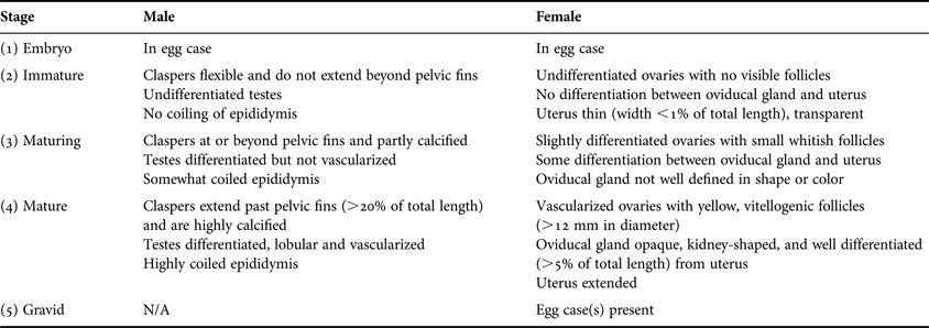
Sex and maturity status were determined in the field by visual inspection of reproductive organs based on Ebert (Reference Ebert2005) (Table 1). Embryos in egg cases were assigned to stage 1. Stages 2 and 3 individuals were classified as immature and maturing, respectively. Specimens identified as maturity stages 4 or 5 were considered mature adults. For males, inner clasper length was measured from the insertion of the clasper near the pelvic fin to the tip. Oviducal gland widths of females were measured at the widest point. Yellow, vitellogenic follicles were identified as mature.
Table 1. Determination of maturity stages by visual inspection for male and female Bathyraja trachura. Modified from Ebert (Reference Ebert2005).

Size- and age-at-maturity were estimated using maturity ogives fit to binomial maturity data (0 = embryo/immature/maturing; 1 = mature/gravid). A logistic regression of the following form was fit to binomial maturity data using iteratively reweighted least squares in R (R Core Team, 2012):
where Y = the probability of being mature and x = TL in mm or age in years. The median size (TL50) and age (Age50) at which 50% of the population was mature was calculated from the resulting regression parameters as −a/b. Ninety-five per cent confidence intervals were also calculated. Sex was incorporated as a factor with or without an interaction term to examine its effect on the probability of maturity. All possible model subsets were evaluated using the AICc as described above.
RESULTS
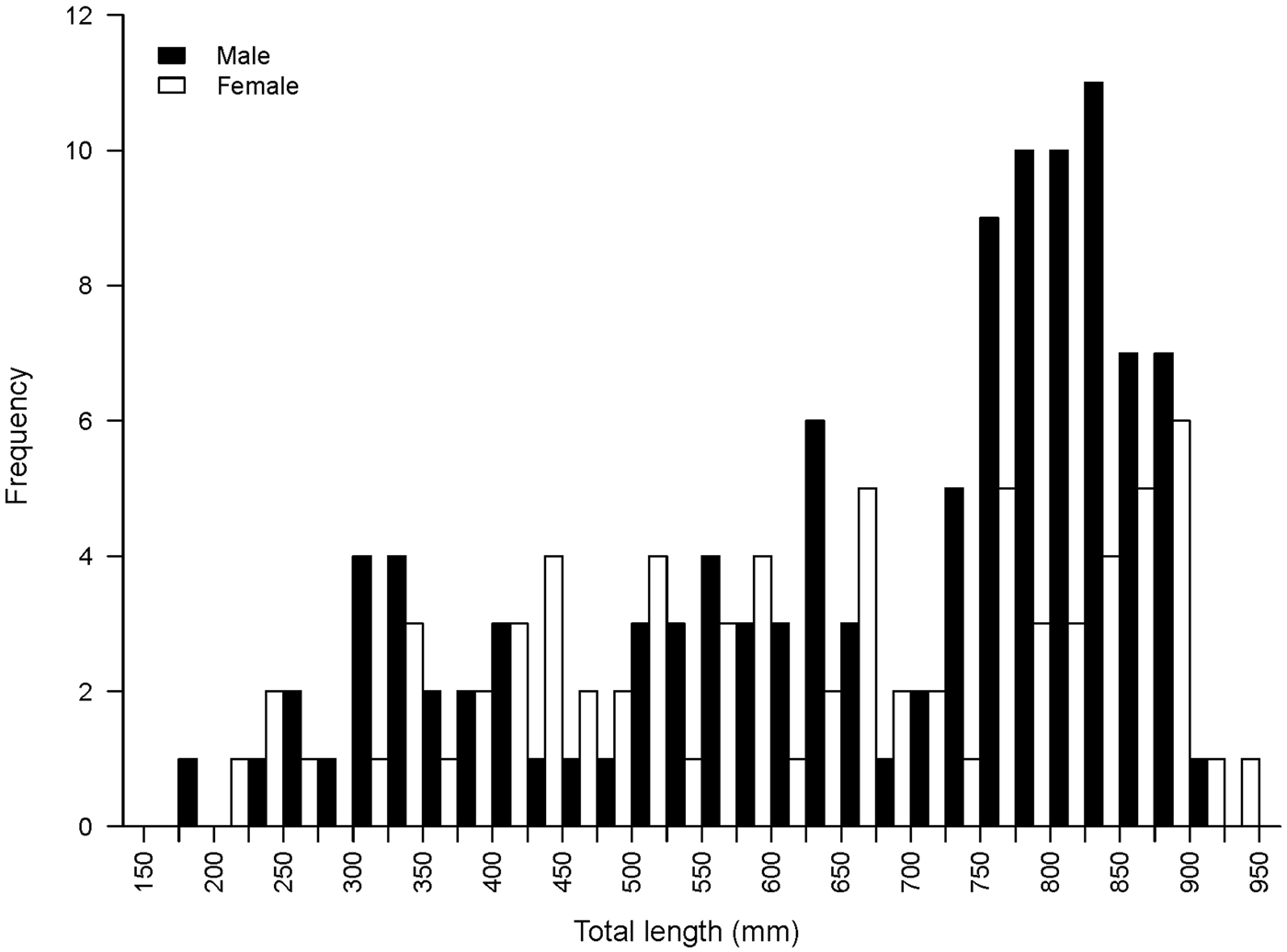
A total of 187 Bathyraja trachura specimens were collected for this study (111 males, 75 females, 1 sex unknown). Skates ranged in size from 182 to 942 mm TL (Figure 1). The smallest female was 204 mm TL and the smallest male 182 mm TL. The largest female was 942 mm TL and the largest male 918 mm TL.

Fig. 1. Size–frequency histogram of male (N = 111) and female (N = 75) Bathyraja trachura sampled from the eastern Bering Sea.
Based on AICc values, regression analysis indicated that the optimal DW–TL relationship included DW, sex and the DW–sex interaction term (N = 182; Table 2). The AICc difference between the optimal model and the regression including only DW as an explanatory variable (ΔDW =28.16) suggested an effect of sex on this relationship and was indicative of sexual dimorphism in disc shape, with males becoming more ‘bell-shaped’ than females upon maturation. The DW–TL relationship was described for both sexes as follows:
Table 2. Parameter estimates for the regression model describing the relationship between disc width (DW) and total length (N = 182).

SE, standard error; *, indicates interaction term.
Age determination
Final age estimates were determined from 142 specimens (86 males, 55 females, 1 sex unknown). Of the original 154 samples collected and prepared for ageing, 12 sections (7.8%) were excluded from analysis due to problems with processing, indiscernible banding patterns or lack of agreement of independent age estimates. Growth bands consisted of wide translucent bands separated by narrow opaque bands (Figure 2). Banding patterns were not visible across the intermedialia in most specimens; therefore, band counts were based on the corpus calcareum. Observed ages ranged from 0 to 36 yr, with a maximum age estimate of 35 yr (827 mm TL) for males and 36 yr (889 mm TL) for females. The largest male (918 mm TL) and female (942 mm TL) had 34 and 31 band pairs, respectively.

Fig. 2. Vertebral section from a Bathyraja trachura specimen. The arrow signifies the birthmark (age 0). Subsequent black circles indicate opaque bands. This 430 mm female had an estimated age of 10 years.
Precision and error analysis
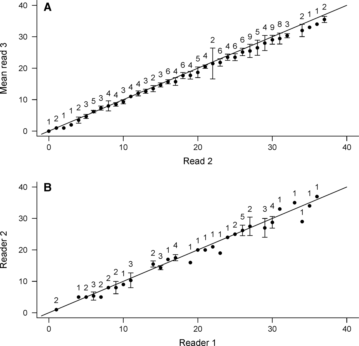
Precision among age estimates was deemed acceptable (CV = 4.5%). Overall percentage agreement was high, with 95.1% of all reads falling within ±3 yr. An age-bias plot indicated no appreciable bias between reads until age 20, after which age estimates became more variable and read 3 produced consistently lower estimates (Figure 3A); the Evans–Hoenig test of symmetry also suggested bias (χ2 = 35.36, df = 5, P < 0.001). Though differences in age estimates were generally small, they occurred in the same direction, with read 3 producing slightly lower band pair counts than read 2.

Fig. 3. Age bias plot between (A) independent reads of Bathyraja trachura vertebral sections (N = 142) by the primary study reader and (B) between readers (N = 55). The 45o line represents 1:1 agreement between band counts. Error bars indicate 95% confidence intervals. Sample sizes are indicated above each age-class.
Inter-reader agreement among age estimates indicated consistency in band pair interpretation (CV = 5.5%). Most reads (92.7%) agreed within ±3 yr and all within ±5 yr. Both age bias plots (Figure 3B) and the Evans–Hoenig test of symmetry (χ2 = 7.11, df = 4, P = 0.13) provided no evidence of appreciable bias between readers.
Growth parameter estimation
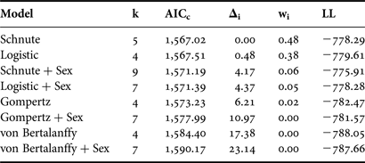
The general form of the Schnute model and the logistic model with common parameter estimates for both sexes were well supported based on the available data (Δi < 2; Table 3). Both versions of the von Bertalanffy as well as the Gompertz including separate parameter estimates for each sex had little to no support (Δi > 10). Incorporating separate parameter estimates for males and females did not improve fit over the model using common parameter estimates for any individual growth curve (Table 3); therefore sexes were pooled for final curve fitting (Table 4). While the Gompertz model did produce biologically reasonable estimates (Table 4), it was not as strongly supported based on AICc values (ΔGompertz = 6.21).
Table 3. Relative goodness-of-fit for each candidate growth model for Bathyraja trachura from the eastern Bering Sea. Models are ranked from best to worst fitting. +Sex indicates the incorporation of separate parameter estimates for males and females; all other models included common parameter estimates for both sexes.

k, total number of regression parameters; AICc, second-order Akaike information criterion; Δi, Akaike difference; wi, Akaike weight; LL, log likelihood.
Table 4. Growth model parameters for Bathyraja trachura based on age estimates from vertebral sections. All models were parameterized as special cases of the general Schnute (Reference Schnute1981) growth model. More commonly presented parameter estimates are also included. Ninety-five per cent bootstrap confidence intervals for each parameter are indicated in parentheses below when relevant. All lengths presented are given in mm.

a, a constant (yr−1) describing the relative rate of the relative growth rate; b, a dimensionless constant describing the incremental relative rate of the relative growth rate; l 1, estimated length at age 1; l 2, estimated length at age 30; L ∞, asymptotic total length; L 0, length at birth; t 0, theoretical time at which the fish would have a length of 0 mm.
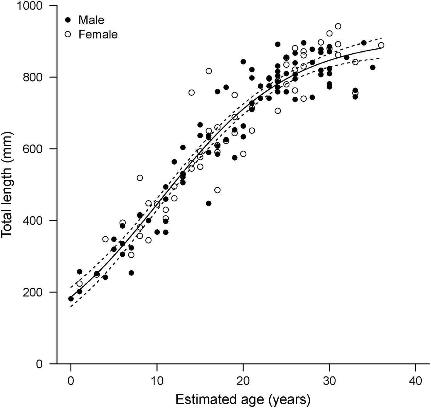
The general Schnute model was technically the best fitting with the absolute lowest AICc value (Table 3). However, it produced less realistic parameter estimates than the logistic model, which was indistinguishable in terms of fit (Δi < 2; Burnham & Anderson, Reference Burnham and Anderson2002). The Schnute model produced an inflated estimate of L 0 =213 mm TL. The reported birth size of the species is approximately 160 mm TL (Ebert, Reference Ebert2003), and the sole specimen with an estimated age of 0 yr in this study had a TL of 182 mm. It also resulted in the lowest estimate of L ∞ = 871 mm TL. While the confidence bounds of the parameter estimates did include more reasonable values, parameter estimates for the logistic model were closer to known values. Therefore, the logistic model was deemed the most appropriate description of growth based on both statistical fit and biological plausibility (Figure 4).

Fig. 4. Logistic growth model fitted to length-at-age data derived from band pair counts in vertebral sections (N = 142) for combined sexes of Bathyraja trachura from the eastern Bering Sea. Dotted lines indicate 95% bootstrap confidence intervals.
Maturity
Maturity status was assigned to 111 males at the time of collection. Roughly half of the males sampled were mature (N = 52; 46.8%). The smallest mature male measured 710 mm TL and the largest immature male 821 mm TL. Inner clasper lengths ranged from 9 to 231 mm (N = 111; TL: 182–918 mm); all mature males had inner clasper lengths greater than 160 mm.
A little more than a quarter of the 75 females collected were mature (N = 20; 26.7%), six of which were gravid. The TL of the smallest mature and largest immature female was 740 mm and 880 mm, respectively. Oviducal gland widths ranged from 3 to 71 mm (N = 63; TL: 249–942 mm); all mature females had oviducal widths greater than 22 mm.
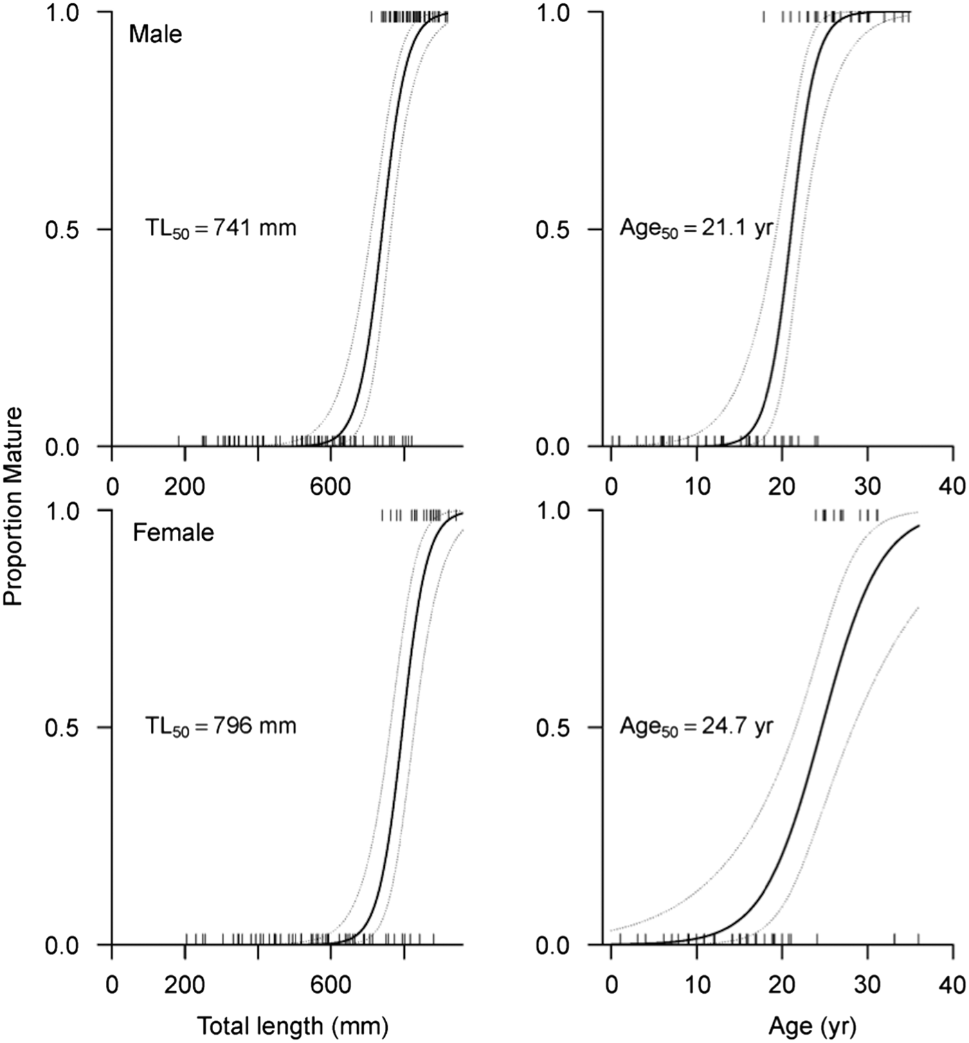
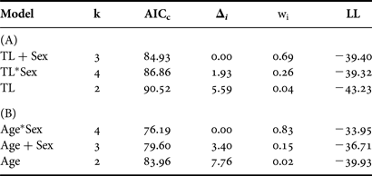
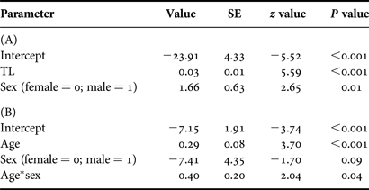
According to the optimal logistic regression model based on AICc values (N = 186; Table 5), the probability of maturity-at-size and -age depended on sex, suggesting difference between males and females. Males matured at smaller sizes and ages than females (Table 6; Figure 5). Based on maturity ogives, TL50 was estimated at 741 mm (95% CI: 710–764 mm) for males and 796 mm (95% CI: 762–828 mm) for females. In terms of age, males and females attained maturity at 21.1 yr (95% CI: 19.4–22.5 yr) and 24.7 yr (95% CI: 21.6–28.3 yr), respectively.

Fig. 5. Estimated probability of maturity-at-size and -age based on maturity ogives for male and female Bathyraja trachura from the eastern Bering Sea. Rug plots indicate individual skates. The median size- (TL50) and age-at-maturity (A50) for each sex is indicated. Dashed lines correspond to 95% confidence intervals.
Table 5. Relative goodness-of-fit for each candidate size-at-maturity model based on (A) total length (TL) and (B) age. Models are ranked from best to worst fitting.

k, number of parameters; AICc, second-order Akaike information criterion; Δi, AICc difference; wi, Akaike weight; LL, log likelihood; +, indicates incorporation of a factor; *, indicates incorporation of an interaction term.
Table 6. Parameter estimates for the optimal model describing the relationship between maturity and (A) total length (TL) and (B) age.

SE, standard error; *, indicates interaction term.
DISCUSSION
The maximum age estimate for Bathyraja trachura from the EBS (36 yr) is among the highest reported for a skate species to date, with corresponding growth coefficients among the lowest (Cailliet & Goldman, Reference Cailliet, Goldman, Carrier, Musick and Heithaus2004; Gallagher et al., Reference Gallagher, Nolan and Jeal2005; Gedamke et al., Reference Gedamke, DuPaul and Musick2005; Sulikowski et al., Reference Sulikowski, Kneebone, Elzey, Jurek, Danley, Howell and Tsang2005; Frisk & Miller, Reference Frisk and Miller2006; Licandeo et al., Reference Licandeo, Lamilla, Rubilar and Vega2006; Davis et al., Reference Davis, Cailliet and Ebert2007; Ebert et al., Reference Ebert, Smith, Haas, Ainsley and Cailliet2007, Reference Ebert, Maurer, Ainsley, Barnett and Cailliet2009; Gburski et al., Reference Gburski, Gaichas and Kimura2007; Natanson et al., Reference Natanson, Sulikowski, Kneebone and Tsang2007; Arikhipkin et al., Reference Arikhipkin, Baumgartner, Brickle, Laptibehousky, Pompert and Shcherbich2008; Ainsley et al., Reference Ainsley, Ebert and Cailliet2011). Overall, age estimates and growth coefficients for B. trachura are most similar to those reported for other deep-dwelling bathyrajid species from the EBS (Table 7). Several studies have suggested that size is linked with life history correlates in skates and therefore may be indicative of a species' potential susceptibility to overexploitation (Dulvy et al., Reference Dulvy, Metcalfe, Glanville, Pawson and Reynolds2000; Frisk et al., Reference Frisk, Miller and Fogarty2001; Dulvy & Reynolds, Reference Dulvy and Reynolds2002). In terms of the Alaskan skate assemblage, it appears that longevity, and hence vulnerability, may scale with depth rather than species' size. This trend has been previously observed among deep-water bony fish and chondrichthyans (Cailliet et al., Reference Cailliet, Andrews, Burton, Watters, Kline and Ferry-Graham2001; García et al., Reference García, Lucifora and Myers2008) and may be related to the reduced metabolic rates of deep dwellers (Childress, Reference Childress1995). For Alaskan bathyrajids that have been aged to date, slope-dwelling species live longer and mature later than those that inhabit the shelf.
Table 7. Summary of available age, growth and maturity data for members of the Alaskan skate assemblage. Three parameter von Bertalanffy growth function parameters are presented for the sake of comparison. Habitat type was based on Ormseth et al. (Reference Ormseth, Matta, amd Hoff, Aydin, Clausen, Conners, Conrath, Dalton, DiCosimo, Echave, Goldman, Hanselman, Heifetz, Hoff, Honkalehto, Ianelli, Kotwicki, Lauth, Lowe, Lunsford, McKelvey, Matta, Nichol, Ormseth, Rodgveller, Rooper, Spencer, Spital, Spies, Stockhausen, TenBrink, Thompson, Tribuzio, Wilderbuer and Wilkins2010). All lengths presented are in cm; ages are in yr. Median size- and age-at-maturity estimates are presented separately for each sex (female estimate/male estimate).

TLmax, maximum observed total length; Agemax, maximum observed longevity; TL50, median total length at maturity; Age50, median age at maturity; L ∞, theoretical asymptotic length; k, von Bertalanffy growth coefficient; t 0, theoretical age at zero length.
Banding patterns in B. trachura were relatively difficult to interpret due to the poor vertebral calcification typical of deep-water elasmobranch species (Cailliet et al., Reference Cailliet, Andrews, Burton, Watters, Kline and Ferry-Graham2001; Gennari & Scacco, Reference Gennari and Scacco2007). The full histological approach has been used in only a handful of studies due to equipment, time and cost requirements (Ishiyama, Reference Ishiyama1951; Natanson & Cailliet, Reference Natanson and Cailliet1990; Natanson, Reference Natanson1993; Natanson et al., Reference Natanson, Sulikowski, Kneebone and Tsang2007). However, the enhancement of banding patterns and subsequent reduction in the difficulties associated with ageing rendered the more time- and cost-intensive histological process worthwhile for B. trachura.
Despite the difficulties experienced with vertebral interpretation, age estimates were comparable between readers and precision was high. The lack of bias between study readers indicated consistency of band pair interpretation in vertebral sections. The bias exhibited by the primary study reader (M.V.W.) was likely due to the reader becoming increasingly familiar with the species' banding patterns with subsequent reads. Inter-reader precision and bias analyses and final age estimates for the EBS population were based on the primary reader's third count; therefore, the observed bias was deemed inconsequential in light of the lack of bias between readers.
Maturity
Bathyraja trachura matures relatively late in life, with females maturing at greater sizes and ages than males, a pattern often reported among skates (Gallagher et al., Reference Gallagher, Nolan and Jeal2005; Gedamke et al., Reference Gedamke, DuPaul and Musick2005; McFarlane & King, Reference McFarlane and King2006; Licandeo & Cerna, Reference Licandeo and Cerna2007). Both sexes reached TL50 at over 70% of their maximum observed size, which falls within the range observed for other skates (Ebert, Reference Ebert2005; Ebert et al., Reference Ebert, Compagno and Cowley2008b; Frisk, Reference Frisk, Carrier, Musick and Heithaus2010; Ainsley et al., Reference Ainsley, Ebert and Cailliet2011). Median age-at-maturity occurred at approximately 69% of the observed maximum age for females and 59% for males. This supports the results of other studies suggesting that skates have a protracted juvenile stage in comparison with most other elasmobranchs (Cortés, Reference Cortés2000; Ebert, Reference Ebert2005; Frisk, Reference Frisk, Carrier, Musick and Heithaus2010).
Median size-at-maturity estimates reported in this study for B. trachura were similar to those previously reported for males, but were larger for females. Ebert (Reference Ebert2005) determined that females (TL50 = 735 mm TL) matured at smaller sizes than males (TL50 = 755 mm TL) in the EBS. However, sample sizes of both sexes were considerably smaller than in the present study. In both studies, maturity classifications were made at sea and based solely on visual assessment; as a result, the potential for misclassification of maturity cannot be excluded. For example, the largest immature female from this study was the oldest observed specimen and may have been reproductively inactive rather than immature (Ebert, Reference Ebert2005). Future studies should incorporate histological assessment of reproductive tracts to avoid misclassifications, which may cumulatively skew estimates of the size- and age-at-maturity.
Latitudinal variability
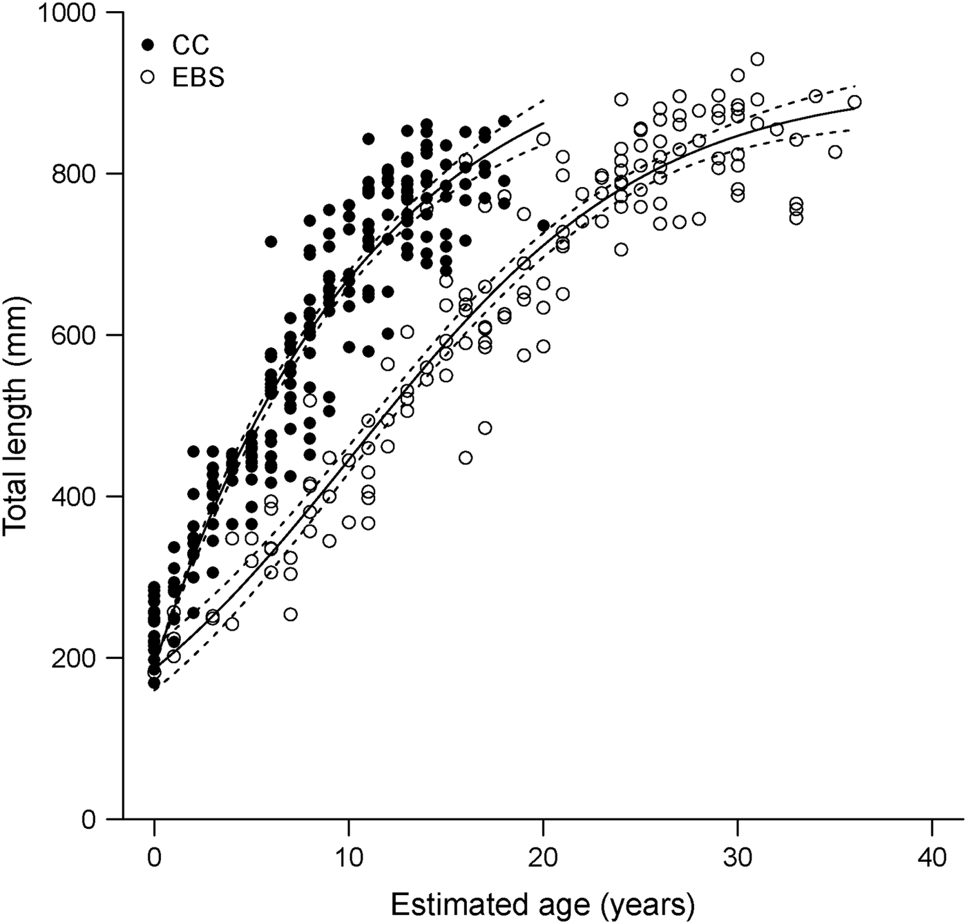
The results of this study may indicate a latitudinal pattern in size and growth for the species, with individuals from the EBS reaching higher maximum ages and growing more slowly than previously reported for specimens collected from the CC (Davis et al., Reference Davis, Cailliet and Ebert2007). The maximum observed age estimate based on vertebral sections for specimens collected from the EBS was 16 yr older than that reported for the CC by Davis et al. (Reference Davis, Cailliet and Ebert2007). Based on the resulting growth curves derived in the two regional studies, B. trachura in the CC have a higher growth rate and consequently reach larger sizes-at-age than in the EBS (Figure 6). Such latitudinal and regional patterns in life histories have often been documented in chondrichthyan fish (Yamaguchi et al., Reference Yamaguchi, Taniuchi and Shimizu1998; Lombardi-Carlson et al., Reference Lombardi-Carlson, Cortés, Parsons and Manire2003; Neer & Thompson, Reference Neer and Thompson2005; Frisk & Miller, Reference Frisk and Miller2006; Licandeo & Cerna, Reference Licandeo and Cerna2007; McPhie & Campana, Reference McPhie and Campana2009).

Fig. 6. Regional growth models fitted to length-at-age data derived from band pair counts in vertebral sections for Bathyraja trachura from the eastern Bering Sea (EBS, N = 142; this study) and California Current ecosystems (CC, N = 214; Davis et al., Reference Davis, Cailliet and Ebert2007). Dotted lines indicate 95% bootstrap confidence intervals.
The results presented do provide evidence of difference in growth between ecosystems; however, it is important to note that these estimates are not directly comparable due to the different vertebral preparation techniques used in both studies. Vertebral sections in this study were prepared using a histological technique; sections from the previous study were examined unstained. Given the difficulties associated with ageing this species, histological preparation of samples used in the earlier study would likely result in slightly higher age estimates; age estimates based on histological sections were 5 yr higher, on average, than those based on unstained sections from the same individuals for EBS specimens (M. Winton, unpublished data). Although the differences reported herein may be inflated as a result, maximum age estimates based on unstained sections from the EBS (M. Winton, unpublished data) were still 10 yr older than those reported by Davis et al. (Reference Davis, Cailliet and Ebert2007). Observed regional differences were also unlikely to be due to interpretation error. Comparison of band pair counts for a subset of vertebrae used in the earlier study (Davis et al., Reference Davis, Cailliet and Ebert2007) indicated no bias between the two study readers (M. Winton, unpublished data).
Previously reported spatial differences in life history parameters of marine species have been attributed to differences in environmental factors such as temperature (Parsons, Reference Parsons1993; Yamaguchi et al., Reference Yamaguchi, Taniuchi and Shimizu2000; Walker, Reference Walker2007), prey availability (Yamaguchi et al., Reference Yamaguchi, Taniuchi and Shimizu2000), exploitation rates (Sosebee, Reference Sosebee2005) and discrete breeding populations (Tovar-Ávila et al., Reference Tovar-Ávila, Walker and Day2007). Of the potential factors listed above, environmental differences are likely the most plausible for this species, although the possibility of genetically discrete populations cannot be excluded due to lack of available data. Temperature is strongly related to growth in fish (Neuheimer & Taggart, Reference Neuheimer and Taggart2007); long-term but small-scale changes in temperature have been linked to corresponding changes in the growth rate of several deep-dwelling teleost species (Thresher et al., Reference Thresher, Koslow, Morison and Smith2007). Bottom temperature values at the depths B. trachura inhabits are 4–5oC higher in the CC than the EBS (Keller et al., Reference Keller, Horness, Simon, Tuttle, Wallace, Fruh, Bosley, Kamikawa and Buchanan2007a, Reference Keller, Simon, Horness, Wallace, Tuttle, Fruh, Bosley, Kamikawa and Buchananb, Reference Keller, Horness, Fruh, Simon, Tuttle, Bosley, Buchanan, Kamikawa and Wallace2008; Lauth, Reference Lauth2011), suggesting that temperature may play some role in the differences observed between regions.
Management implications
Given that several elasmobranch species exhibit seemingly random banding patterns that are not directly related to time (Natanson & Cailliet, Reference Natanson and Cailliet1990; Natanson et al., Reference Natanson, Wintner, Johansson, Piercy, Campbell, De Maddalena, Gulak, Human, Fulgosi, Ebert, Hemida, Mollen, Vanni, Burgess, Compagno and Wedderburn-Maxwell2008), demographic analyses and management actions based on the age estimates reported herein will be inherently characterized by a high degree of uncertainty until validation of age estimates is achieved. The use of incorrect ages and resulting growth rates in demographic analyses can lead to errors in estimates of natural mortality rates, population growth rates and management actions based upon those estimates (Beamish & McFarlane, Reference Beamish and McFarlane1983). Therefore, longevity estimates and any models or management actions based upon unvalidated age estimates should be interpreted with caution.
Cortés (Reference Cortés2002) proposed a ‘fast–slow’ continuum of shark life-history characteristics based on the results of age-structured life table and Leslie matrix analyses. Species at the fast end of the continuum were characterized by fast growth, early maturity, short life span and high productivity. Species at the slow end exhibited slow growth, late maturity, high longevity and consequently low productivity. Bathyraja trachura is among the longest-lived, latest maturing and slowest growing species reported in the Alaskan skate assemblage to date (Table 7; McFarlane & King, Reference McFarlane and King2006; Ebert et al., Reference Ebert, Smith, Haas, Ainsley and Cailliet2007, Reference Ebert, Smith and Cailliet2008a, Reference Ebert, Maurer, Ainsley, Barnett and Cailliet2009; Gburski et al., Reference Gburski, Gaichas and Kimura2007; Matta & Gunderson, Reference Matta and Gunderson2007; Ainsley et al., Reference Ainsley, Ebert and Cailliet2011). Thus, in relative terms, B. trachura falls near the slow end of the spectrum proposed by Cortés (Reference Cortés2002) and will likely be less resilient to fishing pressure than its shelf-dwelling congeners at the faster end of the continuum. Differences in growth parameters observed between the CC and EBS may indicate the presence of distinct populations of B. trachura in the eastern North Pacific and should be taken into account when developing regional skate management plans. Future studies should seek to produce validated age and maturity estimates throughout the species' range in the eastern North Pacific to obtain a more complete idea of intra-specific variability in these essential fisheries parameters.
ACKNOWLEDGEMENTS
This project would not have been possible without the cooperation of the NMFS Alaska Fisheries Science Center (AFSC), Northwest Fisheries Science Center (NWFSC), the Alaska Department of Fish and Game and other members of the Pacific Shark Research Center (PSRC). We would especially like to thank Lyle Britt, Sarah Gaichas, Jerry Hoff, Beth Matta, Jay Orr and Duane Stevenson from the AFSC, and Keith Bosley, Erica Fruh, Aimee Keller, Victor Simon and Dan Kamikawa from the NWFSC. Ken Goldman (ADFG) and PSRC members Joe Bizzarro, Chanté Davis, Brooke Flammang, Heather Robinson and Wade Smith participated on survey cruises and provided invaluable assistance with sampling. Chanté Davis provided access to her data to make the ecosystem comparison portion of this study possible. This research was conducted under IACUC protocol 801.
FINANCIAL SUPPORT
Funding for this project was provided by the North Pacific Research Board (M.W., graduate student research award), (D.E., G.C., project number 715). Additional funding was provided by NOAA/NMFS to the National Shark Research Consortium and the Pacific Shark Research Center (D.E., G.C.); the David and Lucille Packard Foundation (M.W., graduate student award); and the Dr Earl and Ethel M. Myers Oceanographic and Marine Biology Trust (M.W., graduate student award). This is North Pacific Research Board contribution # 452.

