2.1. Direct numerical simulations

Three-dimensional DNS of the turbulent flow around the square cylinder are performed with the ONERA compressible solver FastS (Mary & Sagaut Reference Mary and Sagaut2002; Dandois, Mary & Brion Reference Dandois, Mary and Brion2018). The three-dimensional computational domain is formed by a two-dimensional circle of radius $50 D$ in the $\boldsymbol {x}=(x,y)^{\mathrm {T}}$ plane, centred around the square cylinder, which is extruded in the spanwise homogeneous direction $z$ with length $L_z=4 D$. The two-dimensional mesh consists of approximately $2.6 \times 10^{5}$ grids points and $N_z=960$ planes uniformly discretise the spanwise direction. Periodic boundary conditions are applied in the spanwise direction. Homogeneous free-stream conditions are enforced at the outer boundaries, where only the horizontal velocity component (parallel to upper and lower cylinder surfaces) is non-zero and equal to $U_{\infty }$. The simulation is run close to the incompressible flow regime at $M=0.1$ enforcing no-slip conditions at the cylinder surface. In the following, all quantities are non-dimensionalised based on the reference length $D$ and free-stream parameters $U_{\infty }$, $\rho _{\infty }$. The DNS time step is $\Delta t_{DNS} = 3.3188 \times 10^{-4}$, which corresponds to a maximal Courant–Friedrichs–Lewy number of approximately $0.7$. More details about this DNS solver are provided in Dandois et al. (Reference Dandois, Mary and Brion2018), Mary & Sagaut (Reference Mary and Sagaut2002) and Franceschini et al. (Reference Franceschini, Sipp and Marquet2020).

Obtained unsteady three-dimensional velocity fields $\boldsymbol {u}$ can be decomposed as

(2.1)\begin{equation} \boldsymbol{u}(\boldsymbol{x},z,t) = \bar{\boldsymbol{u}}_{r}(\boldsymbol{x},t) + \boldsymbol{u}^{\prime}(\boldsymbol{x},z,t), \end{equation}

where $\bar {\boldsymbol {u}}_{r}$ is the statistically averaged two-dimensional velocity field of interest while $\boldsymbol {u}^{\prime }$ refers to the associated three-dimensional deviation, not used in the following. Then, it is assumed that $\bar {\boldsymbol {u}}_{r}$ can be extracted from DNS velocity fields $\boldsymbol {u}$ by averaging instantaneous snapshots in the spanwise direction according to

(2.2)\begin{equation} \bar{\boldsymbol{u}}_{r}(\boldsymbol{x},t) = \frac{1}{L_z} \int_{0}^{L_z} \boldsymbol{u}(\boldsymbol{x},z,t) \, {\rm d}z \sim \frac{1}{N_z} \sum_{k=1}^{N_z} \boldsymbol{u}(\boldsymbol{x},z=k \Delta z,t), \end{equation}

where $\Delta z \sim 0.004$ is the uniform discretisation step in the spanwise direction. This spatial average well approximates the statistical average if the spanwise extent $L_z$ of the computational domain and the number of planes $N_z$ are large enough. This two-dimensional field extracted from DNS will be used as reference solution (hence the subscript $r$), first to assess the accuracy of the standard URANS simulation methods in § 2.4, and will then form the targeted flow that we aim to reconstruct based on sparse observations thanks to the nudging method in § 3. To complete the description of this reference dataset, it is obtained by downsampling the DNS snapshots every $63$ time steps. The time interval $\Delta t_{r}$ between snapshots in this reference dataset is thus $\Delta t_{r} = 63 \times \Delta t_{DNS} = 0.0209$ convective time units.

2.2. Unsteady Reynolds-averaged Navier–Stokes simulations

Rather than extracting the temporal variation of the spatially averaged flow from DNS simulations, one may rather estimate the latter through the two-dimensional URANS equations which are supplemented with a turbulence model to take into account the effect of the non-resolved component. The two-dimensional resolved velocity ($\bar {\boldsymbol {u}}$) and pressure ($\bar {p}$) fields then satisfy the following (incompressible) flow equations:

(2.3)\begin{equation} \left.\begin{gathered} \frac{\partial \bar{\boldsymbol{u}}}{\partial t} + (\bar{\boldsymbol{u}} \boldsymbol{\cdot} \boldsymbol{\nabla}) \bar{\boldsymbol{u}} + \boldsymbol{\nabla}\bar{p} - \boldsymbol{\nabla}\boldsymbol{\cdot} \left[ 2\left( Re^{{-}1}+ \nu_t(\tilde{\nu}) \right) \boldsymbol{\nabla}_{{s}} \bar{\boldsymbol{u}} \right] = \boldsymbol{0} , \\ \boldsymbol{\nabla}\boldsymbol{\cdot} \bar{\boldsymbol{u}} = 0, \end{gathered}\right\} \end{equation}

where $\boldsymbol {\nabla }_{{s}} \bar {\boldsymbol {u}}$ refers to the symmetric part of the velocity gradient and $\nu _t$ denotes the turbulent eddy viscosity. Here, the latter is determined using the Spalart–Allmaras model (Spalart & Allmaras Reference Spalart and Allmaras1994), where the following governing equation for the intermediate eddy-viscosity-like variable $\tilde {\nu }$ is solved:

(2.4)\begin{equation} \frac{\partial \tilde{\nu}}{\partial t} + (\bar{\boldsymbol{u}} \boldsymbol{\cdot} \boldsymbol{\nabla}) \tilde{\nu} = s(\tilde{\nu},\bar{\boldsymbol{u}}). \end{equation}

The source term $s$ accounts for the production, dissipation and diffusion terms for $\tilde {\nu }$. Details about the present implementation of the Spalart–Allmaras model are provided in Franceschini et al. (Reference Franceschini, Sipp and Marquet2020).

The URANS equations (2.3)–(2.4) are discretised in space using the finite-element method implemented in the software FreeFEM++ (Hecht Reference Hecht2012). Second-order polynomial elements are employed for the velocity field, while first-order elements are considered for the pressure and eddy-viscosity variables. For the relatively high Reynolds number flow of the present contribution ($Re=22\,000$), streamline-upwind Petrov–Galerkin (SUPG) (Brooks & Hughes Reference Brooks and Hughes1982) and grad-div (Olshanskii et al. Reference Olshanskii, Lube, Heister and Löwe2009) stabilisations are implemented. The rectangular computational domain is sketched in figure 1(a) with an inlet located at $x=-10$, an outlet at $x=15$ and top and bottom planes at $y=10$ and $y=-10$, respectively. Remaining details of figure 1(a) will be discussed later when introducing the nudging approach. The unstructured mesh, shown in figure 1(b), consists of triangles with a total of 46 228 nodes. At the inlet, the boundary condition $(\bar {u},\bar {v},\tilde {\nu })=(1,0,0)$ is imposed. At the cylinder surface, the no-slip boundary condition $\bar {\boldsymbol {u}}=\boldsymbol {0}$ is enforced in conjunction with $\tilde {\nu } = 0$. The conditions ${\partial \tilde {\nu }}/{\partial x}= 0$ and $2(Re^{-1}+\nu _t)\boldsymbol {\nabla }_{{s}}\bar {\boldsymbol {u}} \boldsymbol {\cdot } \boldsymbol {n} - \bar {p} \boldsymbol {n} = \boldsymbol {0}$ are used at the outlet, where $\boldsymbol {n}$ denotes the normal vector. At the top and bottom boundaries, symmetry conditions are imposed according to $({\partial \bar {u}}/{\partial y}, \bar {v},{\partial \tilde {\nu }}/ {\partial y})=\boldsymbol {0}$.

Figure 1. (a) Sketch of the computational domain $\varOmega$ for URANS simulations, where red dots denote positions $(\boldsymbol {x}_{k})_{k=1 \dots M}$ of velocity measurements in the internal domain $\varOmega _{I}$ (bounded by the red frame). These so-called nudging points are uniformly separated in both directions by a spacing distance $\Delta s$. The domain that is external to the measurement area is denoted as $\varOmega _{E}$. (b) Typical triangular mesh used for the standard and nudged URANS simulations around a square cylinder.

Time integration is performed in a fully implicit way based on a second-order accurate finite-difference approximation of the time derivative. A quasi-Newton method is used to solve the resulting nonlinear problem at each iteration. The time step of URANS simulation is denoted by $\Delta t$. Results of the standard simulations presented in § 2.4 are obtained with $\Delta t = \Delta t_{r}$, i.e. matching the time interval of the reference dataset. For nudged URANS simulations in § 3, the value of $\Delta t$ will be equal to the time interval of datasets (not necessarily the reference dataset) inserted into the simulations through the feedback term. By varying the sampling of these datasets, we will thus modify the time step $\Delta t$.

2.3. Temporal and spectral errors

We introduce in this paragraph various mathematical definitions for assessing errors between the reference dataset and the output of the standard or nudged URANS simulations. Note that the latter have not yet been introduced, but we will use the same notation for denoting the corresponding variables in both simulations. In the following, both standard and nudged URANS solutions may be referred to as the estimated flow, while the field $\bar {\boldsymbol {u}}_r$ which is extracted from DNS in (2.2) is referred to as the reference flow, as mentioned above. Definitions of the instantaneous and time-averaged errors are introduced in this section before considering the spectral error based on a spectral proper orthogonal decomposition (SPOD) analysis of the data.

The instantaneous error field $e(\boldsymbol {x},t)$ between the estimated velocity field $\bar {\boldsymbol {u}}$ and the reference one $\bar {\boldsymbol {u}}_{r}$ is defined as

(2.5)\begin{equation} e(\boldsymbol{x},t)=\left({(\bar{u}_{r} -\bar{u})^{2}+( \bar{v}_{r} -\bar{v})^{2}}\right)^{{1}/{2}}. \end{equation}

The instantaneous and time-averaged global errors are then respectively defined as

(2.6a,b)\begin{equation} E(t)=\int_{\varOmega} e(\boldsymbol{x},t)^{2} \, {\rm d}\boldsymbol{x}, \quad \langle E \rangle = \frac{1}{T_{e}} \int_{t_i}^{t_i+T_{e}} E(t) \, {\rm d}t , \end{equation}

where $\varOmega$ denotes the entire computational domain, $t_i>0$ is an arbitrary time that is chosen to avoid transient effects (occurring in $[0,t_i]$) and $T_{e}$ refers to the considered time window for averaging the instantaneous global error. Note that the time average is denoted $\langle \cdot \rangle$, and thus $\langle \bar {\boldsymbol {u}}\rangle$ is the time-averaged velocity field of the estimated flow. Its error compared with the time-averaged reference velocity $\langle \bar {\boldsymbol {u}}_{r}\rangle$ is then defined as

(2.7)\begin{equation} e_{\langle \bar{\boldsymbol{u}} \rangle } (\boldsymbol{x}) = \left(\left( \langle \bar{u}_r \rangle -\langle \bar{u} \rangle \right)^{2} + \left( \langle \bar{v}_r \rangle - \langle \bar{v} \rangle \right)^{2}\right)^{{1}/{2}}. \end{equation}

To better understand the unsteady effect, a spectral analysis of the data is performed which relies on the SPOD described in Towne et al. (Reference Towne, Schmidt and Colonius2018). Taking a temporal series of velocity snapshots as inputs, the SPOD analysis provides a set of SPOD modes $\boldsymbol {\varPhi }=(\varPhi _{u},\varPhi _{v})^{\textrm {T}}$ that each oscillate at a single non-dimensional frequency (Strouhal number) $St=f D/U_{\infty }$. Each frequency corresponds to a set of normalised SPOD modes ($\int _{\varOmega } \boldsymbol {\varPhi }^{*} \boldsymbol {\varPhi } \,\textrm {d}\varOmega = 1$, where the asterisk denotes the Hermitian transpose) ranked by their kinetic energy $\lambda$, that are the eigenvalues of the cross-spectral density tensor which is estimated from snapshots. In the following, we will focus on the dominant SPOD modes, namely which are associated with the largest eigenvalue, for frequencies of interest. Denoting hereinafter the SPOD modes of the reference and URANS solutions as $[\lambda _{r},\boldsymbol {\varPhi }_{r}]$ and $[\lambda,\boldsymbol {\varPhi }]$, respectively, a spectral error field may be defined as

(2.8)\begin{equation} \varPhi_e=\left(\left( \sqrt{\varPhi_{u,r}^{*} \varPhi_{u,r}} - \sqrt{\varPhi_{u}^{*} \varPhi_{u}}\right)^{2} + \left( \sqrt{\varPhi_{v,r}^{*} \varPhi_{v,r}} - \sqrt{\varPhi_{v}^{*} \varPhi_{v}}\right)^{2}\right)^{{1}/{2}}. \end{equation}

In the following, the dynamical content of standard and nudged URANS simulations will thus be assessed and compared with the reference solution through their frequency contents, the kinetic energy of the dominant SPOD modes and the shape of the latter through (2.8).

2.4. Comparisons between standard URANS and DNS

A preliminary URANS simulation is performed to obtain a periodic evolution of the aerodynamic coefficients. It allows us to determine an instant which minimises the discrepancy between the lift coefficients computed from URANS and DNS simulations. The flow field at that instant is then used as initial condition $t=0$ for the URANS simulation that is discussed below. By doing so, the DNS and URANS solutions are initially phased in time and we can thus properly compare the temporal evolution of the error between the two.

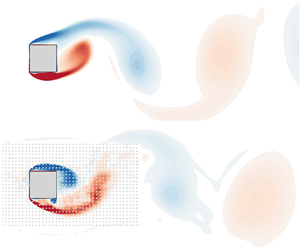
Figure 2 provides a first comparison of the flow extracted from DNS (figure 2a,b) and estimated by the URANS equations (figure 2c,d). The instantaneous vorticity contours are shown in figures 2(a) and 2(c) for $t=50$. In both cases, we observe that large-scale clockwise (blue) and counter-clockwise (red) vortices are shed in the wake of the square cylinder. Small-scale structures are also visible in the reference flow field shown in figure 2(a). In the upper and lower shear layers, emerging from the leading edge corners of the cylinder, they correspond to two-dimensional roll-up structures associated with KH instabilities. In the wake, they interact with the large-scale vortices of the von Kármán VS. Such small-scale structures are clearly absent in the estimated vorticity field that is shown in figure 2(c). Large-scale and small-scale structures are associated with different parts of the Fourier spectra displayed in figure 2(b,d), which are obtained from the streamwise velocity $u$ monitored at a grid point located in the upper shear layer, at $(x,y)=(0.25,0.75)$ (green dot in figure 2a,c). The large-scale periodic VS is associated with several peaks, one at the fundamental frequency $St_{VS}=U_{\infty } f_{VS} / D$ (indicated in both figures by the vertical dashed lines) and the others at multiples of the fundamental frequency, i.e. $k St_{VS}$ with $k\geqslant 2$. The fundamental frequency is $St_{VS} = 0.137$ for the DNS simulation and $St_{VS}= 0.126$ for the standard URANS simulation. The small-scale structures that are observed in the shear layers in the reference snapshot (figure 2a) correspond to a high-frequency broadband bump which is centred around $St_{KH}\approx 4.384$, as indicated by the vertical dotted line in figure 2(b). This high-frequency bump is absent in the spectrum of the URANS signal, displayed with the black curve in figure 2(d). This confirms that the present standard URANS simulation does not capture the emission of KH vortices in the shear layers, at least in a self-sustained way, which will be further discussed at the end of this section.

Figure 2. Results for (a,b) reference (DNS) and (c,d) estimated (standard URANS) flows. (a,c) Instantaneous spanwise vorticity field $\bar {\omega }_z$ at $t=50$, where black iso-curves denote $\left \langle \bar {u} \right \rangle =0$. (b,d) Fourier spectrum of the streamwise velocity at the green monitor point in panels (a,c) (full black line). For the sake of comparison, the DNS spectrum is duplicated in panel (d) with the grey curve. Vertical dashed and dotted lines indicate the low-frequency peak associated with large-scale VS ($St_{VS}=0.137$ for DNS while $St_{VS}=0.126$ for URANS) and the high-frequency bump linked to KH instabilities ($St_{KH}=4.384$ for DNS), respectively.

Although the URANS simulation well approximates the periodic VS phenomenon, the difference between Strouhal numbers noticed above is responsible for desynchronisation of the wake flow as illustrated in figure 3. The instantaneous vorticity fields displayed in figures 3(a–c) and 3(d–f) for DNS and URANS simulations, respectively, seem to be in phase after two VS periods (a,d), but, after four shedding cycles (b,e), large vortex structures observed in URANS snapshots clearly lag behind corresponding structures in DNS snapshots. After $19.5$ periods (c,f), the two solutions are out of phase by a half-wavelength. This desynchronisation of the large-scale structures results in large values of the instantaneous local error in the wake of the cylinder, as illustrated by figure 3(g–i). The temporal evolution of the instantaneous global error $E(t)$ in (2.6a,b) is reported in figure 3(j) from $t=0$ to $t=200$, which corresponds to a time window of $26$ VS periods. The error $E(t)$ increases during the first $20$ periods ($0 \leqslant t \leqslant 150$), in agreement with the previous observations, before slightly decreasing. All the above findings are thus related to the lack of synchronisation between reference and estimated flows, which originates from the misprediction of the fundamental frequency $St_{VS}$ by URANS. This may already justify the need of sequential data assimilation for full flow reconstruction, as only phasing an initial condition from data is not sufficient in the present case to correctly track the reference flow.

Figure 3. Instantaneous vorticity fields of (a–c) the reference flow $\boldsymbol {\bar {u}}_{r}$ (DNS) and (d–f) estimated flow $\bar {\boldsymbol {u}}$ (standard URANS) at times (a,d) $t=15$, (b,e) $t=30$ and (c,f) $t=150$. (g–i) Instantaneous error fields $e(\boldsymbol {x},t)$ between the reference and estimated flows (definition in (2.5)) at the corresponding instants. (j) Temporal evolution of the global error $E(t)$ (see (2.6a,b)), where the bottom axis reports the (non-dimensional) time while the top axis reports the number of low-frequency cycles determined as $t/\tau _{VS}=t \, St_{VS}$ with $St_{VS} = 0.137$. The grey circles indicate times $t=15$, $30$ and $150$.

The statistical and dynamic discrepancies between estimated and reference flows are further examined in the following, where we first consider the time average of these flows. The streamwise velocity of the time-averaged reference (DNS) and estimated (URANS) flows are depicted in figures 4(a) and 4(b), respectively, while the associated discrepancy field $e_{\langle \bar {\boldsymbol {u}} \rangle }(\boldsymbol {x})$ in (2.7) is displayed in figure 4(c). Interestingly, the mean flows agree qualitatively well, and the error field $e_{\langle \bar {\boldsymbol {u}} \rangle }(\boldsymbol {x})$ reaches overall significantly lower values than the discrepancy field $e(\boldsymbol {x},t)$ for the instantaneous flow in figure 3(g–i), at least in the near wake. Largest errors are observed in the shear layers that emerge from the cylinder upstream corners. The recirculation region, which is delineated by black curves, is slightly larger for the estimated flow ($L=0.55$) compared with that of the reference flow ($L=0.45$). Substantial errors are also visible in the far wake where streamwise velocity is overestimated by URANS.

Figure 4. (a,b) Streamwise component of the time-averaged (a) reference flow $\langle \bar {\boldsymbol {u}}_{r} \rangle$ (DNS) and (b) estimated flow $\langle \bar {\boldsymbol {u}} \rangle$ (standard URANS). (c) Associated discrepancy field $e_{\langle \bar {\boldsymbol {u}} \rangle }$ as defined in (2.7). In panels (a,b), black curves correspond to contours of zero streamwise time-averaged velocity, which delineate the recirculation region.

The SPOD decompositions of the reference and estimated flows are both performed by considering as input $8420$ snapshots that are sampled at $\Delta t_{r}=0.021$ in a time interval of around $176$ convective times. Using the Matlab implementation provided by Towne et al. (Reference Towne, Schmidt and Colonius2018), this series is typically divided in three overlapping bins, each bin containing approximately $4200$ instantaneous snapshots, and overlapping by $50\,\%$ of their size. The time interval of a bin is thus around $88$ convective time units.

The SPOD analysis of the VS phenomenon as predicted by DNS and standard URANS is first illustrated in figure 5. Spectra of the most energetic SPOD modes for a low-frequency range ($0 \leqslant St \leqslant 1$) as functions of Strouhal number $St$ are reported in figure 5(b). DNS and URANS results are denoted by black and light grey dots, respectively. As in the Fourier analysis of figure 2, several peaks are observed at the fundamental frequency $St_{VS}=0.137$ of the VS phenomenon and at frequencies corresponding to second and third harmonics at $St_{VS,2}=0.261$ and $St_{VS,2}=0.398$, respectively. Frequencies of URANS modes (grey peaks) are slightly lower, peaking at $St_{VS}=0.126$, $St_{VS,2}=0.261$ and $St_{VS,2}=0.386$. Streamwise velocity contours of the imaginary part of the dominant DNS and URANS SPOD modes for the fundamental frequency $St_{VS}$ are displayed in figures 5(a) and 5(c), respectively. Both modes are phased so that they reach their maximum amplitude at the monitor point indicated by the green dot, which is the same as in figure 2. Their spatial structure is typical of modes corresponding to the alternate shedding of vortices in the wake, with a streamwise wavelength equal to ${\sim }4$ cylinder lengths. Furthermore, we show in figure 5(d) the so-called modal error field $\varPhi _e(\boldsymbol {x})$, which is defined in (2.8). Dominant errors are observed in boundary and shear layers, as well as in the near-wake region, which may be related to the slightly longer recirculation region predicted by URANS.

Figure 5. SPOD analysis of the VS phenomenon in the reference (DNS) and estimated (standard URANS) flows: streamwise velocity contours of the imaginary part of the dominant (a) DNS and (c) URANS SPOD modes for the fundamental frequency $St_{VS}$. Modes are phased so that each of them reaches its maximum value at the green monitor point. (b) Spectra showing the largest eigenvalue $\lambda$ as a function of the frequency $St$ in the low-frequency range $0 \leqslant St \leqslant 1$ for DNS (black curve) and URANS (grey curve). The vertical lines indicate low-frequency peaks at $St_{VS}=0.137$ and their harmonics for DNS results. The modal discrepancy field $\varPhi _e$ in (2.8) between the modes in panels (a,c) is reported in panel (d).

Figure 6(b) shows the spectrum of the most dominant SPOD modes corresponding to high-frequency fluctuations. A broadband peak centred around $St_{KH}=4.384$ is clearly visible in the DNS spectrum (black) but not in the URANS one (grey). In order to prevent modes from being corrupted by numerical oscillations in regions of decreased grid resolution, we limit the domain that is considered for SPOD targeting KH phenomena to $-1.5< x<1.5$ and $-1.5< y<1.5$. Furthermore, we consider $1440$ snapshots at a sampling rate of $\Delta t_{r}=0.021$ in a time interval of around $30$ convective times using $6$ overlapping bins, each containing approximately $33$ KH cycles. In order to better visualise convective small-scale instabilities originating from the front edge of the cylinder, a magnification of the upper-side shear layer in figure 6(a) shows the real part of transverse velocity contours for the dominant SPOD mode from DNS results at $St_{KH}=4.384$. Typical wavelengths of these structures are around $0.25$, i.e. a quarter of the cylinder's length. Similar spatial structures are also observed on the lower side of the cylinder, but of much weaker magnitude. As expected when considering the spatial symmetry of the time-averaged flow, a second SPOD mode with spatial structures predominant on the lower-side shear layer is also obtained but associated with a slightly lower kinetic energy.

Figure 6. (a) Contours of transverse velocity fluctuations are shown for the real part of the dominant SPOD mode of DNS that is associated with KH instabilities ($St_{KH}=4.384$, only captured with DNS). (b) Spectra showing the largest eigenvalue $\lambda$ as a function of the frequency $St$ in the high-frequency range $1 \leqslant St \leqslant 7$. Black and light grey curves correspond to DNS and URANS results, respectively.

As the present standard URANS results do not include such structures, one may suspect the Spalart–Allmaras model to be here too dissipative for self-sustained KH instabilities, as discussed in the introduction. Following proposals in Menter et al. (Reference Menter, Garbaruk, Smirnov, Cokljat and Mathey2010), one may wonder if the Spalart–Allmaras model may at least allow the emergence of KH phenomena from sustained disturbances in the present case. This is investigated through figure 7, showing SPOD results for a URANS calculation, where uniform white noise is injected at $(x,y)=(-0.4,0.6)$ (black dot in the figure). More specifically, the spectrum range of the white noise is limited to $St \geqslant 0.5$ in order to avoid interference with low-frequency VS. Independent realisations of this white noise affect both the streamwise and transverse velocity components at $(x,y)=(-0.4,0.6)$, and the associated standard deviation is $5\times 10^{-3}$. Qualitatively, the results in figure 7 exhibit minor sensitivity with respect to small changes in the amplitude and location of the noise source (not shown here for the sake of brevity). From this punctual disturbance, panels (a,b) confirm the development of KH-like structures. These figures, which may be compared with the reference mode in figure 6(a), correspond to dominant SPOD modes at $St=3.454$ and $St=St_{KH}=4.384$. We can observe significantly increased energy content at these frequencies, especially for $St=3.454$, comparing spectra of perturbed (dark grey curve) and unperturbed (light grey curve) URANS simulations in figure 7(d). On the other hand, higher frequencies ($St \geqslant 5$) are not sustained by the model and the corresponding fluctuations remain localised around the source of white noise, as illustrated by figure 7(c), which reports the dominant SPOD mode at $St=6.510$. While these results do not necessarily agree with the DNS ones on a quantitative basis, they confirm the ability of the URANS equations in frequency selection and in developing shear-layer instabilities. These findings thus support the relevance of employing the present RANS model in the following data assimilation procedure even for completing reference measurements for the estimation of KH phenomena.

Figure 7. (a–c) Contours of transverse velocity fluctuations are shown for the real part of the dominant SPOD mode at (a) $St=3.454$ (vertical dashed line in panel (d)), (b) $St=St_{KH}=4.384$ (vertical full line in panel (d)) and (c) $St=6.510$ (vertical dash-dotted line in panel (d)) for a URANS calculation in which white noise is injected at the black dot. (d) Spectra showing the largest eigenvalue $\lambda$ as a function of the frequency $St$ in the high-frequency range $1 \leqslant St \leqslant 7$. Black and light grey curves correspond to DNS and unperturbed URANS results, respectively, while the dark grey curve refers to the URANS calculation with white noise.

Previously discussed SPOD results for DNS and (unperturbed) standard URANS are summarised in table 1.

Table 1. Time-averaged and unsteady characteristics of the flow obtained with DNS and standard URANS simulations. The first two columns report the maximal lift variation and time-averaged drag coefficients, respectively. The remaining columns report the dominant eigenvalue $\lambda$ for various frequencies $St$ from the SPOD analysis, considering the fundamental harmonic for the von Kármán VS, its second (${VS,2}$) and third (${VS,3}$) harmonics, and the dominant frequency for the broadband emission of KH vortices.

3.1. Data assimilation methodology

3.1.1. Nudged equations and measurements

Nudging allows a dynamic adjustment of the estimated flow through the addition of a feedback term in the URANS momentum equations in (2.3), which is directly proportional to the discrepancies between flow measurements denoted $\boldsymbol {m}$ and the estimated velocity field at the measurement locations. The intensity of this feedback term is adjusted through a parameter called $\alpha$. The estimated velocity field, which is now denoted $\bar {\boldsymbol {u}}_{\alpha }$, satisfies the so-called nudged equations

(3.1)\begin{equation} \frac{\partial \bar{\boldsymbol{u}}_{\alpha}}{\partial t} + (\bar{\boldsymbol{u}}_{\alpha} \boldsymbol{\cdot} \boldsymbol{\nabla}) \bar{\boldsymbol{u}}_{\alpha} + \boldsymbol{\nabla}\bar{p}_{\alpha} - \boldsymbol{\nabla}\boldsymbol{\cdot} \left[ 2\left( Re^{{-}1}+\nu_t(\tilde{\nu}_{\alpha}) \right) \boldsymbol{\nabla}_{{s}} \bar{\boldsymbol{u}}_{\alpha} \right] = \alpha \, \mathcal{H}^{{{\dagger}}} [\boldsymbol{m}-\mathcal{H}(\bar{\boldsymbol{u}}_{\alpha})], \end{equation}

which are supplemented by the divergence-free condition in (2.3) and the Spalart–Allmaras model (2.4) to determine the eddy-viscosity field $\nu _t(\tilde {\nu }_{\alpha })$ in the above equation. The feedback term on the right-hand side involves the measurement operator $\mathcal {H}$, which acts on the estimated velocity field $\bar {\boldsymbol {u}}_{\alpha }$ and returns a vector $\mathcal {H}(\bar {\boldsymbol {u}}_{\alpha })$ in the measurement space. Further details about the measurement operator and its adjoint $\mathcal {H}^{{\dagger} }$ are provided below. Setting $\alpha =0$, one recovers the standard URANS equations, while for $\alpha >0$, the feedback term in the momentum equations drives the estimated flow $\bar {\boldsymbol {u}}_{\alpha }$ towards measurements $\boldsymbol {m}$. The rationale behind the choice of an appropriate value for $\alpha$ is detailed in Appendix A, where minor sensitivity of results is shown as soon as $\alpha >1$. The value $\alpha =100$ is thus chosen in the following nudged URANS simulations. Incidentally, this value appears consistent with the considerations of Di Leoni et al. (Reference Di Leoni, Mazzino and Biferale2020), who established that $\alpha$ should scale as the inverse of the time step of the simulations, which corresponds to $1/\Delta t=50$ for the smallest value of $\Delta t$ investigated here (see § 3.1.2).

In the present study, the measurement operator $\mathcal {H}$ is defined so as to extract the two components of a velocity field at selected spatial locations, thus mimicking the PIV approach but without taking into account any measurement error that may occur in real experiments. These $M$ ‘nudging points’, which are denoted by $\boldsymbol {x}_{k}$ with ${k = 1\dots M}$, are sketched with red dots in figure 1(a). They are chosen to be equidistantly distributed (in both directions) by a spatial distance $\Delta s$ inside a nudging region $\varOmega _I$ which is delimited by the red frame in this figure. The nudging points do not have to coincide with grid nodes. Note that the complementary region is denoted as $\varOmega _{E}$. In the following, the nudging region is fixed to $\varOmega _I=[-1.5,3.5] \times [-1.5,1.5]$ and we will investigate the effect of the spatial sampling $\Delta s$.

The measurements $\boldsymbol {m}$ are here extracted from the reference velocity field $\bar {\boldsymbol {u}}_{r}$ from DNS results (see § 2.1). More precisely, $\boldsymbol {m}$ is defined as

(3.2)\begin{equation} \boldsymbol{m}(t) = \mathcal{H}(\bar{\boldsymbol{u}}_{r}(t)) = \left[ \bar{\boldsymbol{u}}_{r}(\boldsymbol{x}_{1},t) , \ldots , \bar{\boldsymbol{u}}_{r}(\boldsymbol{x}_{M},t) \right]^{\mathrm{T}} = \left[ \boldsymbol{m}_{1}(t), \ldots , \boldsymbol{m}_{M}(t) \right]^{\mathrm{T}}, \end{equation}

where $\boldsymbol {m}_{k}$ is a vector that contains the two velocity components at measurement point $\boldsymbol {x}_{k}$. The size of the data vector $\boldsymbol {m}$ is therefore $2M$. At an instant $t$, the right-hand side term in (3.1) is obtained from the discrepancy between the estimated flow and this data vector, i.e. $[ \boldsymbol {m}-\mathcal {H}(\bar {\boldsymbol {u}}_{\alpha })] = [\boldsymbol {m}_{1}-\bar {\boldsymbol {u}}_{\alpha }(\boldsymbol {x}_{1}) , \ldots,\boldsymbol {m}_{M}-\bar {\boldsymbol {u}}_{\alpha }(\boldsymbol {x}_{M}) ]^{\mathrm {T}}$, and the adjoint measurement operator $\mathcal {H}^{{\dagger} }$ then allows us to transform this discrepancy vector of size $2M$ into a field in the model space of pointwise forcings at the same locations $\boldsymbol {x}_k$ according to

(3.3)\begin{equation} \mathcal{H}^{{{\dagger}}} [\boldsymbol{m}-\mathcal{H}(\bar{\boldsymbol{u}}_{\alpha})]=\sum^{M}_{k=1}\delta(\boldsymbol{x}-\boldsymbol{x}_k)\left( \boldsymbol{m}_{k}-\bar{\boldsymbol{u}}_{\alpha}(\boldsymbol{x}_{k}) \right). \end{equation}

The implementation of the observation operator $\mathcal {H}$ and of its adjoint in the present finite-element solver is detailed in Appendix B.

The temporal and spatial methods that are used to discretise the nudging equation (3.1) are similar to those described in § 2.2 for the standard URANS simulations. Note that the feedback term is discretised as an implicit term so as to improve the numerical stability of the algorithm, thus allowing us to choose the time step $\Delta t$ arbitrarily large. For all simulations considered hereinafter, it is assumed that the measurement vector $\boldsymbol {m}(t_i)$ is available at every instant $t_i=i \Delta t$ of the simulation. In other words, we do not have any difference between the time step $\Delta t$ of the simulation and the time interval between measurements. In the following, $\Delta t$ is therefore used to characterise the temporal sampling of a dataset that can be written as

(3.4)\begin{equation} \left[ \boldsymbol{m}(t_1), \ldots , \boldsymbol{m}(T_m) \right], \end{equation}

where $N_{m}$ is the number of measurement vectors and $T_{m}=t_{N_{m}}=N_{m} \Delta t$ is the measurement time (or equivalently here the time window of the simulations). In the next paragraph, we will detail how the spatial sampling $\Delta s$, the temporal sampling $\Delta t$ and the measurement time $T_{m}$ are chosen to define several datasets that are used to assess the nudging method in its ability to improve the fidelity of the estimated flow at different spatial and temporal flow scales.

As final comments on the feedback term in the nudged URANS equations (3.1) in this section, it should first be emphasised that its structure, which involves the discrepancies between measurements and the estimated flow, is typical of that of sequential data assimilation and state estimation techniques. For example, the much more expensive Kalman filter is recovered by replacing the contribution $\alpha \, \mathcal {H}^{{\dagger} }$ with the Kalman gain $\boldsymbol{\mathsf{K}}$ after discretisation (Lewis et al. Reference Lewis, Xie and Popa2008). Second, the role of this feedback term includes phasing and synchronisation with the reference measurements, independently of the presence or not of turbulence model, as would be the case with other sequential approaches. In the present case, it may in addition be interpreted as compensating for deficiencies in the present RANS model. Accordingly, one could wonder if this feedback term could be instead written in a divergence form, which would be more in accordance with the original structure of the URANS equations. This could be achieved in particular if measurements of the Reynolds-stress tensor were available. For the present study, however, we assume that we only have access to observations of the (resolved) velocity field, which may often be the case in practical applications. Furthermore, we do not intend to correct the RANS model itself here, but rather compensate for adverse effects on physical flow structures (e.g. excessive dissipation), focusing on state estimation of the resolved scales only. The present shape of the feedback term is thus fully justified by data assimilation concepts and, again, would be similar in many sequential schemes. While the results in §§ 3.3–3.4 will confirm the relevance and efficacy of the present approach in the vast majority of the following data assimilation experiments, the punctual aspect of the feedback term in (3.1) and (3.3) can, however, be a matter of debate, in particular in the case of very sparse measurements. In § 3.5, interpolant-based nudging will be investigated as an alternative to the present punctual approach to further enhance reconstruction results in some of the sparsest test cases.

3.1.2. Measurement datasets

Three groups of datasets are defined in table 2 to specifically investigate the ability of nudging to accurately estimate low-frequency VS (group VS), high-frequency KH vortices (group KH) and both phenomena (group $\textrm {VS}+\textrm {KH}$). The frequency $St$, period $\tau =1/St$, and typical wavelength $\lambda _{x}$ of the structures that are associated with each flow phenomenon are first recalled in the first four columns of this table. The time interval $\Delta t$ between consecutive measurements and the total time $T_{m}$ of the simulations are then chosen to properly capture one of the two phenomena (VS or KH) or both of them ($\textrm {VS}+\textrm {KH}$). The ratios $\tau /\Delta t$ and $T_m/\tau$, which are indicated in the last two columns, correspond to the number of measurement snapshots per cycle and to the total number of cycles, respectively. They confirm that the temporal resolution and time window of the data assimilation experiments are sufficiently large to capture the physics of interest.

Table 2. Description of three groups of measurement datasets which are named from the targeted flow phenomenon by the nudging approach: the von Kármán VS, the KH vortices and both phenomena ($\textrm {VS}+\textrm {KH}$). Their frequency $St$ and period $\tau =1/St$ as captured by DNS are recalled in the second and third columns, respectively. These dataset groups are characterised by the time interval between consecutive measurements $\Delta t$ (fifth column), the number of measurement snapshots $N_m$ (sixth column) and the total measurement time $T_m$ (seventh column). The last two columns report the number of snapshots per cycle (of the target flow phenomenon) and the total number of cycles.

It may be noted that datasets of group $\textrm {VS}+\textrm {KH}$ combine the temporal resolution of group KH ($\Delta t= 0.021$) and the time window of group VS ($T_{m}\simeq 180$), which makes them sufficiently well resolved for describing the high-frequency shedding of KH vortices ($11$ snapshots per cycle), while also capturing a significant number ($24$) of the low-frequency von Kármán VS cycles. Datasets in this group ($\textrm {VS}+\textrm {KH}$) are therefore characterised by a large number of measurement snapshots ($N_{m} \sim 10^{4}$), which makes them less convenient for parametric studies. They will mainly be used in § 3.2 to demonstrate the ability of the nudging method to reconstruct both phenomena based on measurements that are dense in both time and space.

The influence of the spatial resolution $\Delta s$ on the performance of the data assimilation procedure is mainly investigated using the dataset groups VS and KH in §§ 3.3 and 3.4, respectively. Table 3 summarises the values of spatial sampling $\Delta s$ that are tested for each dataset group. More precisely, it indicates the number of measurement points $N_s=\lambda _{x}/\varDelta _{s}$ that sample the characteristic wavelength $\lambda _{x}$ of the corresponding flow structure. The datasets of group VS cover a wide range of spatial resolutions, from the highest resolution with $128$ points per wavelength when $\Delta s=0.03125$, to the lowest spatial resolution with two points per wavelength for $\Delta s =2$. The spatial resolution covered by the datasets of group KH is more restricted, from $8$ points to only $1$ point per wavelength of KH vortices.

Table 3. Test matrix indicating, for the three dataset groups VS, KH and $\textrm {VS}+\textrm {KH}$ in table 2, the number of measurement points $N_{s} = \lambda _{x}/\Delta s$ that sample the wavelength $\lambda _{x}$ of the corresponding spatial structures (indicated in the fourth column of table 2) when varying the spatial sampling $\Delta s$. For instance, the dataset VS(a) corresponds to $(\lambda _{x}=4.00,\Delta s=0.03125)$, thus $N_s=128$.

3.3. Nudging the low-frequency large-scale structures (dataset group VS)

We now specifically analyse the performance of the nudging approach in the accurate estimation of low-frequency phenomena ($St<1$) using datasets of lower resolution. More specifically, we now consider dataset group VS in table 2, which is characterised by the temporal sampling $\Delta t = 0.209$, this value being $10$ times larger than for the dataset group $\textrm {VS}+\textrm {KH}$ used in § 3.2. Moreover, for most of the datasets in group VS, the spatial sampling $\Delta s$ is also decreased compared with previous results. As summarised in table 3, the investigated values of $\Delta s$ amount to $2 \leqslant N_s \leqslant 128$, where $N_s=\lambda _x/\Delta s$ is the number of nudging points per characteristic wavelength $\lambda _x \sim 4$ of the large-scale vortices.

Figure 11 shows the vorticity fields at $t=50$ and the Fourier spectra of the streamwise velocity at point $(x,y)=(0.25,0.75)$, similarly to figures 2 and 8, which are obtained for nudged URANS simulations with decreasing values of the spatial sampling $\Delta s$. In the Fourier spectra, results corresponding to nudged URANS are displayed with black curves, while the grey curves correspond to results of the reference flow when sampled at $\Delta t = 0.209$, i.e. the temporal sampling of the present dataset. This spectrum is therefore different from the reference spectrum in figures 2 and 8 that corresponds to a temporal sampling ten times smaller, ($\Delta t = 0.021$). Their comparison clearly shows the filtering effect when downsampling the reference flow.

Figure 11. Results for nudged URANS simulations in dataset group VS with spatial spacings (a,b) $\Delta s = 1.66$, (c,d) $\Delta s = 1.5$, (e,f) $\Delta s = 0.5$ and (g,h) $\Delta s = 0.125$. (a,c,e,g) Instantaneous spanwise vorticity field $\bar {\omega }_{z}$ at $t=50$, where black iso-curves denote $\left \langle \bar {u} \right \rangle =0$, while dots refer to nudging points. (b,d,f,h) Fourier spectrum of the streamwise velocity at the green monitor point in panels (a,c,e,g) (full black line), the reference spectrum to recover is also reported (full grey curve). Vertical dashed lines indicate the low-frequency peak associated with large-scale VS.

Let us first examine results obtained with the largest spatial samplings displayed in figure 11(a,b) for $\Delta s = 1.66$ and in figure 11(c,d) for $\Delta s = 1.5$. For $\Delta s = 1.66$, the nudged simulation is not synchronised with the measurement data. The largest amplitude peak is obtained for a frequency that is slightly lower than in the reference simulation (see figure 11b) and is the same as in the standard URANS results ($St_{VS}=0.126$ vs $St_{VS}=0.137$ in the reference simulation). By increasing the spatial sampling of the observations to $\Delta s = 1.5$, the VS frequency of the nudged simulation already locks to the reference frequency (figure 11d). Furthermore, this appears to be true not only for the fundamental frequency $St_{VS}$, but also for its second and third harmonics. For the present set-up, the smallest number of measurement points that is necessary to lock the low frequencies associated with large-scale VS is thus around only $N_s \sim 2.5$ points per characteristic wavelength. However, despite this frequency locking, it may be noticed that the estimated flow is still not perfectly in phase with the reference one for $\Delta s=1.5$, as further discussed in the following. Moreover, the largest amplitude peak is underestimated, as well as the power spectral densities at higher frequencies. Furthermore, as for $\Delta s = 1.66$, the vorticity field in figure 11(c) (as in figure 11a) exhibits undesired small-scale wake-like structures around some nudging points. This appears as one limitation of nudging based on pointwise forcings at the measurement locations in the case of very sparse data. This issue will be revisited and addressed in § 3.5 by modifying the structure of the feedback term in the nudged URANS equations (3.1).

A better flow estimation is obtained by further decreasing the spatial sampling to $\Delta s = 0.5$ (figure 11e,f). The large-scale vortices are now well synchronised with the reference flow (figure 2a) and the dominant peak in the spectrum is almost perfectly recovered. Moreover, the spurious small-scale structures around nudging points that were observed for larger spatial samplings are not visible anymore. Decreasing the spacing between nudging points to $\Delta s = 0.125$ adds more small-scale features to the nudged URANS simulation, as illustrated by figure 11(g), which gets even closer to the reference snapshot of figure 2(a). In addition, the corresponding spectrum in figure 11(h) agrees perfectly well with the downsampled reference one. It may be emphasised that $\Delta s = 0.125$ still corresponds to a much lower resolution compared with that of the mesh that is used in the URANS calculations.

To better assess the frequency locking and phasing effects when varying the number of nudging points, we display in figures 12(a) and 12(b) the frequency of the largest amplitude peak $St_{VS}$ and the phase shift $\phi$, respectively, as a function of $\Delta s$ (and $N_s$). As noticed above, the fundamental frequency of the nudged simulations is equal to that in standard URANS results ($St_{VS}=0.126$) for low spatial resolution ($N_s<2.5$) and locks to the frequency of the reference flow ($St_{VS}=0.137$) for higher spatial spatial resolution ($N_s>2.5$). This frequency locking does not guarantee a perfect flow synchronisation. Indeed, for $2.5 \leqslant Ns \leqslant 5.75$, we observe a significant phase shift between temporal evolutions of the streamwise velocity in nudged and reference solutions at the monitor point in figure 11, which vanishes only for higher spatial resolution ($N_s \geqslant 8$).

Figure 12. (a) Dominant Strouhal number and (b) phase angle with respect to reference results as a function of the spacing between nudging points $\Delta s$, or equivalently the number $N_{s}$ of nudging points per characteristic wavelength, for nudged URANS simulations of dataset group VS. Results are obtained from the Fourier analysis of the signal at the same monitor point as in figure 11. Filled symbols correspond to the case where the estimated shedding frequency is $St_{VS}=0.137$, as in DNS results, while open symbols correspond to $St_{VS}=0.126$, as in standard URANS.

The effect of the spatial resolution of measurement points on the time-averaged global error $\langle {E} \rangle$ in (2.6a,b) is now examined through figure 13(a). In this figure, $\langle {E} \rangle$ is normalised by its value for standard URANS results. For the smallest number of nudging points $N_s=2 \, (\Delta s=2)$, the normalised error is slightly smaller than one, indicating a very weak improvement compared with the standard simulation. When increasing to $N_s=2.66$, i.e. the smallest number of nudging points leading to a frequency locking, the normalised error decreases to $0.3$, which corresponds to an improvement of $70\,\%$ compared with the standard URANS results. Interestingly, for $2.66 \leqslant N_s \leqslant 5.75$, the evolution of the error follows that of the phase shift shown in figure 12(b). In this range of spatial resolution, the decrease of the error is thus strongly related to the decrease of the phase shift noticed before. Finally, for $N_s \geqslant 8$, the time-averaged error reaches a constant value that is close to $0.05$ times the standard URANS error.

Figure 13. Time-averaged errors as a function of the spacing between nudging points $\Delta s$, or equivalently the number $N_{s}$ of nudging points per characteristic wavelength, for nudged URANS simulations of dataset group VS. (a) Total error $\langle E \rangle$ in (2.6a,b), which may be decomposed as the sum of (b) internal $\langle {E_I} \rangle$ (black symbols) and external errors $\langle {E_E} \rangle$ (grey symbols). The reported values are normalised by the total time-averaged error for the standard URANS solution. Filled symbols correspond to the case where the estimated shedding frequency is $St_{VS}=0.137$, as in DNS results, while open symbols correspond to $St_{VS}=0.126$, as in standard URANS.

To assess the extrapolation capability of the nudged simulations, $\langle {E} \rangle$ is decomposed into internal and external components, $\langle {E}_I \rangle$ and $\langle {E}_E \rangle$, corresponding to the errors inside and outside the nudging region, respectively, similarly as in § 3.2. The time-averaged internal and external errors, normalised by the total error of the standard simulation, are displayed as a function of $N_s$ in figure 13(b) using black and grey dots, respectively. We clearly note that the external error is the dominant component, whatever the number of nudging points, as for the dataset $\textrm {VS}+\textrm {KH}$(a) discussed in § 3.2. For a small number of nudging points ($N_s < 5.75$), these two errors are of similar order of magnitude, and they decrease in a similar way when increasing the number of nudging points. This is related to the improved flow synchronisation (frequency locking and phase-shift decrease) which has been previously noticed for that range of spatial resolution and occurs everywhere in the flow. Once the number of nudging points is large enough to perfectly synchronise the flow ($N_s > 5.75$), the internal error strongly decreases unlike the external error that reaches a constant value around $5\,\%$ of the total error obtained by standard URANS simulation. This constant value agrees with the total error in figure 13(a) for $\Delta s \leqslant 0.75$. This irreducible error may be attributed to (turbulence) model errors which limit the extrapolation capability of the nudging approach. Its interpolation capability, i.e. the ability to estimate the flow in between nudging points, is nevertheless very good as the internal error decreases to $10^{-4}$.

Having carefully characterised in time the flow estimations for the dataset group VS, we now analyse these results in the frequency space through SPOD, as performed in previous sections. For the present dataset, SPOD is computed based on overlapping bins that cover approximately $63$ time units corresponding to approximately $9$ VS cycles. The frequency $St_{VS}$ and eigenvalue $\lambda _{VS}$ (kinetic energy) corresponding to the largest amplitude peak (see figure 5b) are shown in figures 14(a) and 14(b), respectively, as a function of the spacing between measurements $\Delta s$. For $\Delta s > 1.5$, the frequency of the nudged mode is equal to that of the URANS mode ($St_{VS}=0.126$), while for $\Delta s \leqslant 1.5$, it locks to the frequency of the reference mode ($St_{VS}=0.137$), in agreement with previous observations deduced from a pointwise temporal signal (figure 12). Figure 14(a) thus confirms the global aspect of frequency locking for $\Delta s \leqslant 1.5$. Examining now the estimated kinetic energy $\lambda _{VS}$ of the dominant SPOD mode at $St_{VS}$ in figure 14(b), it is almost equal to that of the reference mode (dash-dotted line) once the frequency is locked to the reference frequency. Using $N_s=2$ points per wavelength ($\Delta s=2$ in the figure), the kinetic energy is still close to that of the URANS mode (dashed line). But a slight increase to $N_s=2.66$ points ($\Delta s=1.5$) yields an almost perfect agreement with the reference value. Further increasing the number of nudging points (decreasing their spacing $\Delta s$) does not significantly improve the estimation of $\lambda _{VS}$. The spatial structure of the corresponding mode is shown in figure 15(a,c,e,g) for several spatial spacings $\Delta s$. In addition, the corresponding spectral error fields $\varPhi _e$ in (2.8) are reported in figure 15(b,d,f,h). For the SPOD mode associated with the unlocked frequency (figure 15a,b), the largest errors are obtained close to some of the nudging points downstream of the cylinder. They are associated with errors in the cross-stream velocity (not displayed here) since the streamwise velocity is zero on the symmetry axis $y=0$. These specific defects vanish once the frequency is locked to the reference frequency (figure 15c,d). Largest errors are now obtained in between nudging points, in a (red) pocket immediately downstream of the cylinder ($x<1.5$) and in two symmetric (yellow) pockets around $x=2$. Both the shape and the intensity of the errors are actually similar to those for standard URANS (figure 5d). Reducing the spacing between nudging points to $\Delta s=0.5$ (figure 15e,f), these errors decrease in the near wake. One may directly identify for the mode in figure 15(e) a change in the structures around $2 \leqslant x \leqslant 4$ compared with previous cases, these structures being now closer to the ones in the reference mode (figure 5a). However, modal errors are significantly reduced only for spacings $\Delta s \leqslant 0.25$, as well as for the case $\Delta s = 0.125$, which is illustrated in figure 15(g,h). The residual errors in the far wake ($x>8$) are barely modified when further increasing the number of nudging points. Accurately recovering the detailed shape of the dominant SPOD mode associated with VS thus seems to require more spatially dense measurements ($N_s\geqslant 16$ nudging points per characteristic wavelength) compared with the estimation of its frequency and kinetic energy/magnitude ($N_s \sim 2.5$). However, it may be emphasised that the estimation of the shape of such a mode, which is already acceptable with standard URANS (see figure 5), may be considered as only secondary to the correct prediction of associated frequency and kinetic energy. These results from the SPOD analysis agree with the low values for the time-averaged global errors $\langle E \rangle$ that are already reached for $N_s \geqslant 2.66$, i.e. after frequency locking and phasing are achieved, and also with a correct estimation of $\lambda _{VS}$, as discussed previously.

Figure 14. (a) Frequency and (b) kinetic energy of the dominant SPOD mode corresponding to VS as a function of the spatial sampling $\Delta s$ for nudged URANS simulations of dataset group VS. The dashed and dash-dotted horizontal lines in panel (b) correspond to the energy of the SPOD mode for the standard URANS and reference solutions, respectively. The spatial structure of a few modes is displayed in figure 15. Filled symbols correspond to the case where the estimated shedding frequency is $St_{VS}=0.137$, as in DNS results, while open symbols correspond to $St_{VS}=0.126$, as in standard URANS.

Figure 15. SPOD analysis of the VS phenomenon for nudged URANS simulations in dataset group VS with spatial spacings (a,b) $\Delta s = 1.66$, (c,d) $\Delta s = 1.5$, (e,f) $\Delta s = 0.5$ and (g,h) $\Delta s = 0.125$. (a,c,e,g) Streamwise velocity contours of the imaginary part of the dominant SPOD mode for the fundamental frequency $St_{VS}$. While the frequency of the mode in panel (a) is $St_{VS}=0.126$, remaining modes oscillate at $St_{VS}=0.137$. Modes are phased so that each of them reaches its maximum value at the green monitor point. (b,d,f,h) Corresponding modal discrepancy field $\varPhi _e$ in (2.8).

Finally in this section, the quality of the mean flow estimated by the nudged URANS simulations for dataset group VS is discussed. The streamwise mean velocity field is depicted in figure 16(a,c,e,g) for several values of $\Delta s$ and can be compared with the reference and URANS mean flows displayed in figures 4(a) and 4(b), respectively. The corresponding error fields $e_{\langle \bar {\boldsymbol {u}}\rangle }$ in (2.7) are reported in figure 16(b,d,f,h). For the lowest spatial resolution ($\Delta s=1.66$), significant improvement is already observed in the far wake outside of the nudging region, which is remarkable as the fundamental frequency $St_{VS}$ is not locked to the reference one in this case. Once it is locked for $\Delta s=1.5$ (figure 16c,d), the error increases in the near wake, similarly to the spectral error of the SPOD mode in figure 15(d) for the same spacing. This mean-flow error can be decreased by increasing the number of nudging points. Significant improvements may already be identified for $\Delta s=0.5$ (figure 16e,f). For the largest spatial resolution ($\Delta s=0.125$) displayed in figure 16(g,h), the mean-flow error drops below $3\,\%$ in the near and far wake. Only the error in the shear layers cannot be further decreased when increasing the number of nudging points.

Figure 16. Mean-flow results for nudged URANS simulations in dataset group VS with spatial spacing (a,b) $\Delta s = 1.66$, (c,d) $\Delta s = 1.5$, (e,f) $\Delta s = 0.5$ and (g,h) $\Delta s = 0.125$. (a,c,e,g) Streamwise component of the mean flow. Black curves correspond to the isocontours of zero streamwise velocity. (b,d,f,h) Mean-flow error field $e_{\langle \bar {\boldsymbol {u}}\rangle }$ in (2.7). The extent of the nudging region is delineated by black lines.

A more quantitative description of the mean-flow error is provided in figure 17 which displays the spatially integrated mean-flow error $\int _{\varOmega _{\langle \bar {\boldsymbol {u}}\rangle }} e_{\langle \bar {\boldsymbol {u}}\rangle } (\boldsymbol {x})^{2} \,\textrm {d}\boldsymbol {x}$, where $\varOmega _{\langle \bar {\boldsymbol {u}}\rangle }$ is the domain of integration. Figure 17(a) illustrated this global error, divided by the value for standard URANS results, as a function of $\Delta s$ for two domains having the same streamwise extent ($-1.5 \leqslant x \leqslant 12.5$) but different cross-stream ones. Squares correspond to the mean-flow error when integrated in a domain of size $-4 \leqslant y \leqslant 4$, which is identical to the $y$-extension used for the figures. In this case, the global mean-flow error is only moderately decreased (by ${\sim }50\,\%$ or less) even for the smallest value of $\Delta s$. However, when restricting the domain $\varOmega _{\langle \bar {\boldsymbol {u}}\rangle }$ to the extension of the nudging region in the cross-stream direction ($-1.5 \leqslant y \leqslant 1.5$), the global mean-flow error (circles) exhibits a larger decrease for $\Delta s \leqslant 1$, while it remains fairly constant for $\Delta s > 1$. This evolution is better understood by examining the internal (black circles) and external (grey circles) components of this error, which are displayed in figure 17(b). For $\Delta s >1$, the decrease of the external error is actually balanced by the increase of the internal error. These two opposite effects were already visible in figure 16(a–d). For $\Delta s \leqslant 1$, both internal and external mean-flow errors decrease almost monotonically. The external contribution reaches a constant value for $\Delta s \leqslant 0.25$ while the internal one still decreases, which is reminiscent of the evolution of the time-averaged spatially integrated errors in figure 13. To conclude, the nudging approach using the low-frequency dataset also allows for an improvement in the mean-flow prediction, not only inside but also outside of the nudging region. This extrapolation capability is mainly significant for a domain of limited extension in the cross-stream direction, which seems related to the extension of the nudging region and appears to be directly downstream of the latter, according to the present results.

Figure 17. (a) Spatially integrated mean-flow error $\int _{\varOmega _{\langle \bar {\boldsymbol {u}}\rangle }} e_{\langle \bar {\boldsymbol {u}} \rangle } (\boldsymbol {x})^{2} \,\textrm {d}\boldsymbol {x}$ of the nudged URANS simulations of dataset group VS as a function of the spatial sampling $\Delta s$. This integrated error is evaluated over a spatial domain $\varOmega$ that extends in the streamwise direction in the range $-1.5 \leqslant x \leqslant 12.5$ and is restricted in the cross-stream direction to (squares) $-4 \leqslant y \leqslant 4$ or (circles) $-1.5 \leqslant y \leqslant 1.5$. (b) The integrated error in the restricted domain $-1.5 \leqslant y \leqslant 1.5$ is decomposed as the sum of internal (black) and external (grey) errors with respect to the nudging region. Reported values are normalised by the corresponding error of the standard URANS solution.

3.4. Nudging the high-frequency small-scale structures (dataset group KH)

As detailed in § 2.4, DNS results capture the shedding of KH vortices in the shear layers around the cylinder. As illustrated by figure 6, a broadband peak is observed around a frequency of $St=4.384$ in the spectrum obtained by the SPOD analysis, and the dominant SPOD mode is characterised by spatially oscillating structures of wavelength $\lambda _{x}\sim 0.25$ located in the upper shear layer. While such structures are absent in the present standard URANS simulations, their formation could be triggered by sustained perturbations. In this section, we now investigate the potential of the nudging approach in the accurate estimation of these phenomena by using the datasets of group KH (see tables 2 and 3). While datasets in this group generally correspond to higher temporal and spatial samplings compared with previously discussed datasets (group VS in § 3.3), it may be noticed that these resolutions are actually moderate compared with the time and spatial scales that are associated with the KH vortices. The time sampling $\Delta t$ indeed corresponds to approximately $11$ snapshots per KH cycle, while the investigated values of $\Delta s$ amount to a number of nudging points per wavelength of the KH vortices verifying $1 \leqslant N_s \leqslant 8$. Results are here directly analysed based on a SPOD analysis that is adapted to KH phenomena, as performed in § 2.4.

The real part of the transverse component of the dominant SPOD mode at $St_{KH}=4.384$ obtained with nudging is shown in figure 18(a,c,e,g) for the different values of the spatial sampling $\Delta s$ in dataset group KH. SPOD spectra are also displayed in panels (b,d,f,h). The SPOD mode in figure 18(a), already captures fluctuations that are reminiscent of KH structures visible in the reference SPOD mode in figure 6(a). The shape of the estimated mode is already quite close to the reference one for $x \geqslant 0$ (comparisons may also be performed with the mode in figure 18(g) which is very close to the reference one). This is remarkable, as the associated spatial sampling $\Delta s = 0.25$ corresponds to $N_s=1$, i.e. one nudging point per wavelength of coherent vortex structures. This notable result is likely favoured by the ability of the present URANS model to allow the emergence of KH structures from sustained excitation, as demonstrated in § 2.4. The present findings may also be related to the observation in Di Leoni, Mazzino & Biferale (Reference Di Leoni, Mazzino and Biferale2018) that nudging was able to compensate for modelling limitations in the form of badly known physical parameters in the case of rotating homogeneous turbulence.

Figure 18. SPOD analysis of KH phenomena as estimated by nudged URANS simulations for the dataset group KH with (a,b) $N_s=1$ ($\Delta s=0.25$), (c,d) $N_s=2$ ($\Delta s=0.125$), (e,f) $N_s=4$ ($\Delta s=0.0625$) and (g,h) $N_s=8$ ($\Delta s=0.03125$) nudging points per wavelength of the KH instabilities. (a,c,e,g) Real part of the transverse component of the SPOD mode for $St_{KH}=4.384$ and (b,d,f,h) SPOD spectrum for nudged URANS (black), the DNS results (grey) are also reported for the sake of comparison.

However, the spectrum in figure 18(b) indicates significantly underestimated amplitudes of all dominant modes around $St_{KH}=4.384$. In particular, the amplitude $\lambda _{KH}$ of the mode in figure 18(a) corresponds to only ${\sim }4\,\%$ of the reference value. Similarly to the results of figure 7, the nudging approach excites modes that are associated with KH instabilities. Their energy amplification, however, is not large enough to reach sufficient amplitudes, probably because of the eddy viscosity provided by the Spalart–Allmaras model, which dissipates too quickly the energy at that frequency. Increasing the spatial resolution of nudging points leads to increasingly pronounced spectral peaks at $St_{KH}=4.384$, as more energy is introduced to promote KH structures. This can be confirmed in figure 18(c,d) for $\Delta s = 0.125 \, (N_s=2)$. Eventually, the spatial pattern obtained for smaller spatial samplings (see figure 18e,g) becomes even closer to the reference SPOD mode (figure 6a). The good performance of nudging is also evident in the SPOD spectra shown in figures 18(f) and 18(h). A number $N_s=8$ nudging points per KH wavelength (figure 18g,h) thus appears sufficient to satisfactorily predict the kinetic energy of the modes around $St_{KH}=4.384$. In particular, the estimated amplitude $\lambda _{KH}$ corresponds to ${\sim }80\,\%$ of the reference value.

We have shown that applying nudging with sufficiently well-resolved measurement data allows us to correctly estimate KH vortices, which are not captured by the standard URANS equations in a self-sustained way. Similarly as for the estimation of low-frequency phenomena (see § 3.3), it may be emphasised that nudging improves URANS simulations in a ‘global’ sense and is here not simply ‘overruling’ local values in shear layers. This is particularly evident for the case with large spacing between nudging points (see figure 18a), where local maxima and minima in SPOD modes associated with KH instabilities do not coincide with nudging positions.

3.5. Interpolant-based nudging

As previously discussed, the present data assimilation procedure appears efficient in correctly estimating various flow phenomena from limited observations. However, in the case of very sparse data ($\Delta s \geqslant 1.5$), it was noticed that nudging may introduce spurious structures which emerge from the measurement locations, as illustrated by figure 11(a,c). This originates from the localised nature of the feedback term in the nudged URANS equations in (3.1) and (3.3). As an alternative to punctual nudging, we consider in this section the application of interpolant-based nudging as proposed by Azouani, Olson & Titi (Reference Azouani, Olson and Titi2014). In this approach, instead of directly considering the punctual measurements $\boldsymbol {m}(t)$ in (3.2), they are first spatially interpolated to get a more regular representation of the data. The thus obtained field $\tilde {\boldsymbol {m}}(\boldsymbol {x},t)$ may belong to the same function space as the estimated velocity field $\bar {\boldsymbol {u}}_{\alpha }(\boldsymbol {x},t)$. This interpolation process is denoted as

(3.6)\begin{equation} \tilde{\boldsymbol{m}}(\boldsymbol{x},t)=\tilde{\mathcal{I}}(\boldsymbol{m}(t)), \end{equation}

where $\tilde {\mathcal {I}}$ refers to the interpolation operator. As detailed in Appendix B, the interpolation procedure is performed based on a mesh whose nodes coincide with the measurement locations and is thus fully independent of the mesh in figure 1(b), which is used to solve the URANS equations. To enable a consistent comparison with $\tilde {\boldsymbol {m}}(\boldsymbol {x},t)$ without any approximation, one has to pass the estimated velocity field through the same interpolation process. In other words, $\tilde {\boldsymbol {m}}(\boldsymbol {x},t)$ should be compared with $\tilde {\boldsymbol {u}}_{\alpha }(\boldsymbol {x},t)=\tilde {\mathcal {I}}(\mathcal {H}(\bar {\boldsymbol {u}}_{\alpha }(\boldsymbol {x},t)))$, where $\mathcal {H}$ extracts the values of the estimated velocity field at the measurement locations, as detailed in § 3.1.1 and Appendix B. In this framework, the interpolant-based nudged URANS equations may be written as

(3.7)\begin{equation} \frac{\partial \bar{\boldsymbol{u}}_{\alpha}}{\partial t} + (\bar{\boldsymbol{u}}_{\alpha} \boldsymbol{\cdot} \boldsymbol{\nabla}) \bar{\boldsymbol{u}}_{\alpha} + \boldsymbol{\nabla}\bar{p}_{\alpha} - \boldsymbol{\nabla}\boldsymbol{\cdot} \left[ 2\left( Re^{{-}1}+\nu_t(\tilde{\nu}_{\alpha}) \right) \boldsymbol{\nabla}_{{s}} \bar{\boldsymbol{u}}_{\alpha} \right] = \alpha[\tilde{\boldsymbol{m}}- \tilde{\mathcal{I}}(\mathcal{H}(\bar{\boldsymbol{u}}_{\alpha}))]. \end{equation}

Contrary to the previous nudged URANS equations (3.1), the feedback term on the right-hand side of (3.7) is not punctual and may affect the URANS equations in the whole measurement domain $\varOmega _{I}$ in figure 1(a).

Interpolant-based nudging (3.7) is applied in figure 19 for a spacing between measurements $\Delta s=1.5$ and dataset group VS. For the sake of comparison, the results in figure 11(c,d), which have been obtained with punctual nudging for the same case are reproduced in figure 19(a,b). In accordance with theoretical considerations (Azouani & Titi Reference Azouani and Titi2014), the estimated field obtained through interpolant-based nudging (figure 19c) appears much more regular than the one with punctual nudging (figure 19a). This is particularly striking in the measurement domain where the spurious structures that are observed in the punctual case are absent in the flow that is retrieved through interpolant-based nudging. While for $\Delta s=1.5$ punctual nudging already enables frequency locking, as discussed in § 3.3, it appears from the comparison between figures 19(b) and 19(d) that interpolant-based nudging further improves the estimation of the Fourier spectrum of the velocity fluctuations at the monitor point in figure 19(a,c), which is in this case quite far from all measurement points. In addition, the flow that is estimated by interpolant-based nudging is better phased with the reference one, which results in a decrease of the time-averaged global error $\langle E \rangle$ in (2.6a,b) by a factor of $\sim 2.4$ compared with punctual nudging. On the other hand, no significant variation in the quality of the estimation of the mean flow or that of the dominant SPOD mode at $St=St_{VS}$ was noticed between punctual and interpolant-based nudging. This may be consistent with the fact that the spurious structures that are introduced by punctual nudging are partly smoothed out through time average and have less impact on statistical quantities than on instantaneous ones.

Figure 19. Results for nudged URANS simulations in dataset group VS with spatial spacing $\Delta s = 1.5$ where nudging is applied either (a,b) in its standard punctual form or (c,d) through interpolant. (a,c) Instantaneous spanwise vorticity field $\bar {\omega }_{z}$ at $t=50$, where black iso-curves denote $\left \langle \bar {u} \right \rangle =0$, while dots refer to nudging points. (b,d) Fourier spectrum of the streamwise velocity at the green monitor point in panels (a,c) (full black line), the reference spectrum to recover is also reported (full grey curve). Vertical dashed lines indicate the low-frequency peak associated with large-scale VS.

Finally, interpolant-based nudging is applied to dataset group KH for $\Delta s=0.125$. This spacing still corresponds to a low resolution with respect to KH phenomena ($N_{s}=2$ points per characteristic wavelength). The dominant SPOD mode at $St=St_{KH}$ that is estimated by punctual nudging in figure 18(c) is reproduced in figure 20(a) and may be compared with the one that is obtained through interpolant-based nudging in figure 20(b). While both modes are similar in terms of global spectral errors $\int _{\varOmega } \varPhi _{e}(\boldsymbol {x})^{2}\,\textrm {d}\boldsymbol {x}$ (see (2.8)), it appears that the interpolant-based nudging approach has removed any trace of the measurement locations in the SPOD mode, which seems significantly smoother than with punctual nudging. Figure 20(b) even better illustrates the ability of the (nudged) URANS equations in providing an estimation of the spatial structure of the developing KH instabilities in between measurement points.

Figure 20. Real part of the transverse component of the SPOD mode for $St_{KH}=4.384$ for nudged URANS simulations in dataset group KH with $\Delta s=0.125$ where nudging is applied either (a) in its standard punctual form or (b) through interpolant.

While not substantially affecting the statistics of the flow and despite of requiring more implementation work, interpolant-based nudging thus appears as an interesting alternative to punctual nudging to ensure the smoothness of the estimated velocity field in the case of too sparse measurements.

3.6. Modelling and experimental considerations

As discussed in §§ 3.3–3.5, the use of nudging in conjunction with URANS here appears to be an efficient flow estimation approach even when considering moderately dense data with respect to the phenomenon of interest. For both large-scale VS and KH instabilities, with a time interval between measurements that is below one tenth of the considered characteristic period, less than $N_s=3$ nudging points per characteristic wavelength is already enough to correct the frequency content of URANS. The kinetic energy that is associated with the (SPOD) modes that oscillate at the frequencies of interest is also satisfactorily recovered with $N_s=3$ and $N_s=8$ for large-scale VS and KH phenomena, respectively. The detailed shape of these modes may be further adjusted when increasing the measurement spatial density. If one is only interested in mean quantities, a spatial sampling of $\Delta s=0.25$, or equivalently $N_s=4$ if the cylinder size is here considered as the characteristic length, is sufficient to significantly improve the estimation of the mean flow compared with standard URANS for the present flow configuration.

It may be worth emphasising that the present results have been obtained in conjunction with a specific RANS turbulence model, namely the Spalart–Allmaras one. Through the consideration of other models, one could possibly further decrease the requirements in terms of temporal and spatial samplings of the measurements, in particular concerning the estimation of the KH instabilities. As discussed in the introduction and reported in the study of Palkin et al. (Reference Palkin, Mullyadzhanov, Hadziabdić and Hanjalić2016), the use of Reynolds-stress models should enable the prediction of KH phenomena in a self-sustained way. When applying data assimilation to further improve their estimation, it could thus be imagined in this case that fewer nudging points could be required in order to accurately predict the associated kinetic energy. Aside from the choice of the turbulence model in the URANS framework, more generally, it seems worth investigating the use of nudging to enhance the estimation of turbulent flows in conjunction with related modelling approaches, namely hybrid approaches (Sagaut, Deck & Terracol Reference Sagaut, Deck and Terracol2013; Chaouat Reference Chaouat2017) such as scale-adaptive simulations (Menter & Egorov Reference Menter and Egorov2010), partially averaged Navier–Stokes (Girimaji Reference Girimaji2006) or partially integrated transport modelling (Chaouat & Schiestel Reference Chaouat and Schiestel2005), among others. Such approaches generally provide clearer and explicit definitions of the resolved and modelled scales, and thus may disambiguate which aspects, i.e. scales, in reference/experimental data the estimated flow is supposed to recover.

In the perspective of using the current nudging approach in an actual experimental context, it is interesting to note that the above mentioned temporal and spatial resolutions may be considered as quite realistic in an experimental point of view, i.e. if one were to consider performing a PIV experiment of the present flow. Similar to the current nudging procedure, PIV measurements are also typically characterised by regular spatial sampling of measurements within a rectangular-shaped measurement domain. Current state of the art in high frame rate PIV includes cameras with a typical sensor size of roughly $2000$ pixels. Using standard seeding conditions and current processing algorithms, an interrogation window would consist of 16 pixels with 75 % overlap (Raffel et al. Reference Raffel, Willert, Scarano, Kähler, Wereley and Kompenhans2018). The final vector spacing would be $\Delta s_{PIV} = 0.03$, which roughly corresponds to the lowest spatial sampling investigated here. Considering a water-flow experiment and a cylinder size of e.g. $20 \ \textrm {mm}$ (leading to a flow velocity of roughly $1.1\ \textrm {m}\ \textrm {s}^{-1}$), the frequency of shear-layer instabilities would be roughly equal to $230 \ \textrm {Hz}$. The present requirement of acquisition to be performed at a roughly ten times higher frequency (thus $2.3 \ \textrm {kHz}$) is thus also reachable, as a high frame rate PIV system can nowadays operate with full laser energy and camera resolution at frequencies of $2{-}3\ \textrm {kHz}$ minimum.

Note that this remains of course a rapid and preliminary verification. Turning to an actual experiment would raise a number of additional challenges (local spatial averaging due to the PIV interrogation windows, measurement noise, etc.), which will be addressed in future steps. However, it is already quite promising that the amount of data necessary for the nudging method to yield excellent results is at first order compatible with current experimental capabilities.