


1 Introduction
It is established that wall turbulence contains a significant element of coherence. This structural nature of turbulent boundary layers has been the subject of many investigations, and a great deal of effort and progress has been made in understanding the processes that are responsible for the ordered turbulent fluctuations observed in wall-bounded turbulence. Robinson (Reference Robinson1991) provides a comprehensive review of early findings focusing on the coherence in the near-wall and buffer region of the flow, while more recent findings are discussed in Marusic & Adrian (Reference Marusic, Adrian, Davidson, Yukio and Sreenivasan2012) and Herpin et al. (Reference Herpin, Stanislas, Foucaut and Coudert2013). Considerable effort has also been devoted to understanding their self-sustaining mechanisms, with different viewpoints thoroughly discussed by Panton (Reference Panton2001).
Over the last decade, the presence of large-scale motions of the order of the boundary layer thickness has received considerable interest. These motions have been shown to be increasingly energetic at higher Reynolds numbers (Hutchins & Marusic Reference Hutchins and Marusic2007), to exist in both internal and external wall-bounded flows (Monty et al. Reference Monty, Hutchins, Ng, Marusic and Chong2009), to influence interfacial bulging (Falco Reference Falco1977; Adrian, Meinhart & Tomkins Reference Adrian, Meinhart and Tomkins2000) and to carry substantial proportions of Reynolds shear stress and turbulence production (Ganapathisubramani, Longmire & Marusic Reference Ganapathisubramani, Longmire and Marusic2003; Balakumar & Adrian Reference Balakumar and Adrian2007). Further, their effect on the smaller-scale fluctuations in the near-wall region has recently been documented (see, for example, Mathis, Hutchins & Marusic (Reference Mathis, Hutchins and Marusic2009)). Longitudinally, these large-scale structures are known to incline forward at a characteristic angle (Adrian et al. Reference Adrian, Meinhart and Tomkins2000; Marusic & Heuer Reference Marusic and Heuer2007), while laterally their width appears to increase with wall distance (Tomkins & Adrian Reference Tomkins and Adrian2003; Hutchins, Hambleton & Marusic Reference Hutchins, Hambleton and Marusic2005; Lee & Sung Reference Lee and Sung2011), and they appear to exhibit some degree of streamwise–spanwise organisation (Elsinga et al. Reference Elsinga, Adrian, Van Oudheusden and Scarano2010). More recently, the dynamics of these large-scale motions has also been examined through direct numerical simulations, which have access to increasingly higher Reynolds numbers (Flores & Jiménez Reference Flores and Jiménez2010; Hwang & Cossu Reference Hwang and Cossu2010; Lee et al. Reference Lee, Lee, Choi and Sung2014; Lozano-Durán & Jiménez Reference Lozano-Durán and Jiménez2014).

Figure 1. Colour contours of the spanwise velocity fluctuations,
 $v$
, of a turbulent boundary layer at
$v$
, of a turbulent boundary layer at
 $Re_{\unicode[STIX]{x1D70F}}\approx 2500$
. Results are presented on streamwise/spanwise planes acquired (a) at
$Re_{\unicode[STIX]{x1D70F}}\approx 2500$
. Results are presented on streamwise/spanwise planes acquired (a) at
 $z\approx \unicode[STIX]{x1D6FF}$
and (b) in the logarithmic region (
$z\approx \unicode[STIX]{x1D6FF}$
and (b) in the logarithmic region (
 $z\approx 0.1\unicode[STIX]{x1D6FF}$
). The top, middle and bottom rows for each wall-normal location show the same flow field unconditioned and decomposed by the sign of
$z\approx 0.1\unicode[STIX]{x1D6FF}$
). The top, middle and bottom rows for each wall-normal location show the same flow field unconditioned and decomposed by the sign of
 $v$
, i.e.
$v$
, i.e.
 $v$
,
$v$
,
 $v<0$
and
$v<0$
and
 $v>0$
respectively. The black dashed lines in (a) correspond to an inclination angle of
$v>0$
respectively. The black dashed lines in (a) correspond to an inclination angle of
 $\pm 45^{\circ }$
with respect to the flow direction,
$\pm 45^{\circ }$
with respect to the flow direction,
 $x$
, and are only included for illustrative purposes.
$x$
, and are only included for illustrative purposes.
In this study, we focus on the large-scale spatial coherence of the spanwise velocity, which to date is largely unexplored. One distinct feature reported for this velocity component is the large diagonal pattern observed on a plane parallel to the wall at the edge of the boundary layer (Sillero, Jiménez & Moser Reference Sillero, Jiménez and Moser2014). This feature is best described with reference to figure 1(a), which shows a representative snapshot of the spanwise velocity fluctuations,
 $v$
, from the present particle image velocimetry (PIV) experiment at a wall-normal height of
$v$
, from the present particle image velocimetry (PIV) experiment at a wall-normal height of
 $z\approx \unicode[STIX]{x1D6FF}$
. Here, the boundary layer thickness,
$z\approx \unicode[STIX]{x1D6FF}$
. Here, the boundary layer thickness,
 $\unicode[STIX]{x1D6FF}$
, corresponds to the wall distance where the mean streamwise velocity is 99 % of the free-stream velocity. From this velocity field, it is clear that coherent regions of positive and negative
$\unicode[STIX]{x1D6FF}$
, corresponds to the wall distance where the mean streamwise velocity is 99 % of the free-stream velocity. From this velocity field, it is clear that coherent regions of positive and negative
 $v$
appear to be counter-oriented at oblique angles and seem to have spatial extents in excess of
$v$
appear to be counter-oriented at oblique angles and seem to have spatial extents in excess of
 $\unicode[STIX]{x1D6FF}$
. To date, most experimental datasets with direct spatial information have had insufficient spatial domains to clearly visualise this large-scale coherence. Moreover, experiments with large streamwise/spanwise domains generally focus on the logarithmic region of boundary layers (Tomkins & Adrian Reference Tomkins and Adrian2003, and others), where the longest coherent regions of streamwise velocity appear to reside (Hutchins & Marusic Reference Hutchins and Marusic2007). The PIV experiments with very large spatial extents targeted at the logarithmic and wake regions of a boundary layer presented herein offer a promising approach to carefully examine these large-scale motions. It is worth noting that the persistent patterns observed in the
$\unicode[STIX]{x1D6FF}$
. To date, most experimental datasets with direct spatial information have had insufficient spatial domains to clearly visualise this large-scale coherence. Moreover, experiments with large streamwise/spanwise domains generally focus on the logarithmic region of boundary layers (Tomkins & Adrian Reference Tomkins and Adrian2003, and others), where the longest coherent regions of streamwise velocity appear to reside (Hutchins & Marusic Reference Hutchins and Marusic2007). The PIV experiments with very large spatial extents targeted at the logarithmic and wake regions of a boundary layer presented herein offer a promising approach to carefully examine these large-scale motions. It is worth noting that the persistent patterns observed in the
 $v$
coherence at the edge of the boundary layer are largely unaffected by the reference velocity (here based on a Reynolds decomposition (Reynolds Reference Reynolds1894)) as the mean spanwise velocity is nominally zero in a canonical turbulent boundary layer. However, prior works have reported differences in the
$v$
coherence at the edge of the boundary layer are largely unaffected by the reference velocity (here based on a Reynolds decomposition (Reynolds Reference Reynolds1894)) as the mean spanwise velocity is nominally zero in a canonical turbulent boundary layer. However, prior works have reported differences in the
 $u$
coherence based on the reference velocity at the edge of the layer (see Kwon, Hutchins & Monty Reference Kwon, Hutchins and Monty2016). Figure 1(b) reproduces the same velocity field in the logarithmic region, where the diagonal pattern for the spanwise coherence is no longer obvious based on the sign of
$u$
coherence based on the reference velocity at the edge of the layer (see Kwon, Hutchins & Monty Reference Kwon, Hutchins and Monty2016). Figure 1(b) reproduces the same velocity field in the logarithmic region, where the diagonal pattern for the spanwise coherence is no longer obvious based on the sign of
 $v$
(see also Sillero et al.
Reference Sillero, Jiménez and Moser2014). In the present study, we attempt to address whether similar oblique features are still present closer to the wall and how they can be extracted.
$v$
(see also Sillero et al.
Reference Sillero, Jiménez and Moser2014). In the present study, we attempt to address whether similar oblique features are still present closer to the wall and how they can be extracted.
Over the last few decades, attempts to model the large-scale structural features in wall turbulence have received considerable attention, with models based on hairpin or packet-like structures being the most studied (summarised recently by Marusic & Adrian (Reference Marusic, Adrian, Davidson, Yukio and Sreenivasan2012)). For example, the models described by Perry and coworkers (see Perry & Chong Reference Perry and Chong1982; Marusic & Perry Reference Marusic and Perry1995 and Perry & Marusic Reference Perry and Marusic1995) based on the attached eddy hypothesis (Townsend Reference Townsend1976) have been shown to reproduce the general behaviour of flow statistics in wall-bounded turbulence. Recent works have also shown that this model can be used as a tool to aid understanding of structural observations from numerical and experimental work (de Silva, Hutchins & Marusic Reference de Silva, Hutchins and Marusic2016a ), as the eddies used in the model can be prescribed.
Accordingly, encouraged by recent numerical observations by Sillero et al. (Reference Sillero, Jiménez and Moser2014), this study aims to examine the large-scale oblique features of the spanwise coherence in turbulent boundary layers. We begin with a description of the experimental databases in § 2. Section 3 presents conditional correlation analysis of the large-scale spanwise coherence in the wake region and § 4 presents evidence of similar oblique features closer to the wall in the logarithmic region. Thereafter, § 5 describes how these observations relate to the intermittent turbulent bulges at the edge of the boundary layer. Finally, in § 6, we test whether synthetic velocity fields constructed based on the attached eddy model reproduce a similar behaviour in the spanwise coherence to that observed experimentally. We also discuss whether this behaviour is associated with the signature of a collection of self-similar eddies or perhaps due to different possible scenarios.
Throughout this work, the coordinate system
 $x$
,
$x$
,
 $y$
and
$y$
and
 $z$
refers to the streamwise, spanwise and wall-normal directions respectively. Corresponding instantaneous streamwise, spanwise and wall-normal velocities are represented by
$z$
refers to the streamwise, spanwise and wall-normal directions respectively. Corresponding instantaneous streamwise, spanwise and wall-normal velocities are represented by
 $\widetilde{U}$
,
$\widetilde{U}$
,
 $\widetilde{V}$
and
$\widetilde{V}$
and
 $\widetilde{W}$
respectively. Lower case letters
$\widetilde{W}$
respectively. Lower case letters
 $u$
,
$u$
,
 $v$
and
$v$
and
 $w$
correspond to the fluctuating velocity components. Overbars and
$w$
correspond to the fluctuating velocity components. Overbars and
 $\langle \rangle$
denote average quantities and the superscript
$\langle \rangle$
denote average quantities and the superscript
 $+$
refers to normalisation by viscous variables. For example, we use
$+$
refers to normalisation by viscous variables. For example, we use
 $\widetilde{U}^{+}=\widetilde{U}/U_{\unicode[STIX]{x1D70F}}$
for velocity, where
$\widetilde{U}^{+}=\widetilde{U}/U_{\unicode[STIX]{x1D70F}}$
for velocity, where
 $U_{\unicode[STIX]{x1D70F}}$
is the friction velocity.
$U_{\unicode[STIX]{x1D70F}}$
is the friction velocity.
2 Description of the experiments
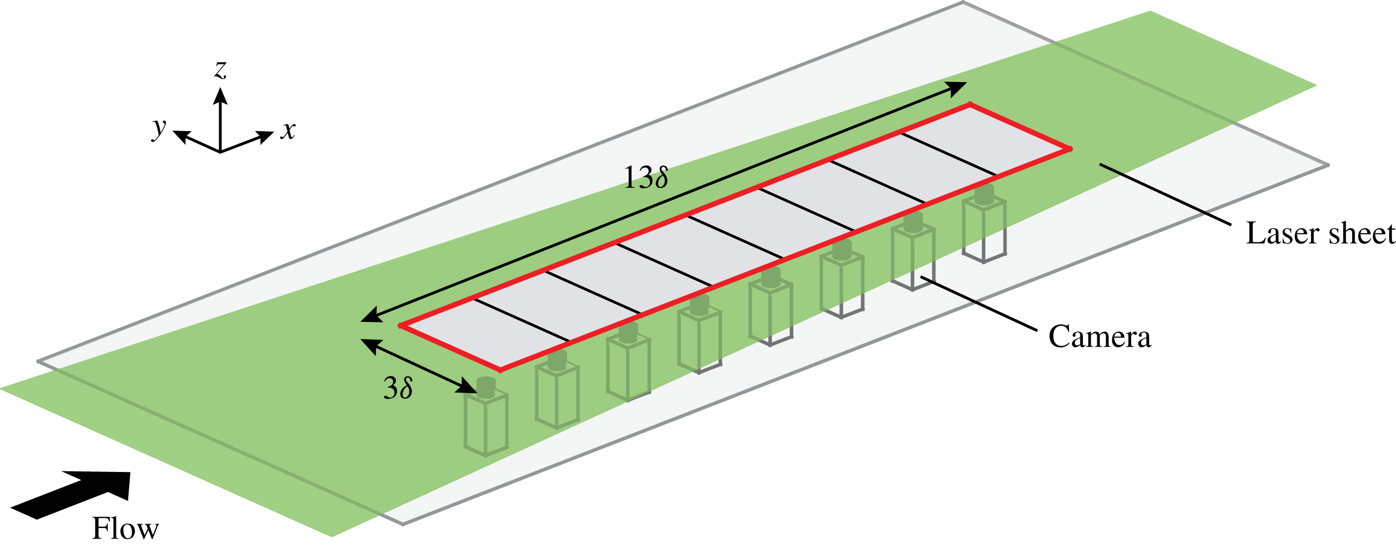
Figure 2. The experimental set-up used to conduct large-field-of-view planar PIV experiments in the HRNBLWT to a capture a streamwise/spanwise (
 $xy$
) plane. The red solid line corresponds to the combined field of view captured from the multicamera imaging system. For the present work, streamwise/spanwise planes are captured in the logarithmic region (
$xy$
) plane. The red solid line corresponds to the combined field of view captured from the multicamera imaging system. For the present work, streamwise/spanwise planes are captured in the logarithmic region (
 $z/\unicode[STIX]{x1D6FF}\approx 0.1$
) and at
$z/\unicode[STIX]{x1D6FF}\approx 0.1$
) and at
 $z/\unicode[STIX]{x1D6FF}\approx 0.4$
, 0.8 and 1.
$z/\unicode[STIX]{x1D6FF}\approx 0.4$
, 0.8 and 1.
The experiments were performed in the High Reynolds Number Boundary Layer Wind Tunnel (HRNBLWT) at the University of Melbourne. The working section of this facility has a large development length of approximately 27 m, permitting high Reynolds numbers to be achieved at relatively low free-stream velocities (Nickels et al.
Reference Nickels, Marusic, Hafez and Chong2005). This provides a uniquely thick boundary layer, resulting in a larger measurable viscous length scale (and hence less acute spatial resolution issues). Unlike prior PIV campaigns in the HRNBLWT (de Silva et al.
Reference de Silva, Gnanamanickam, Atkinson, Buchmann, Hutchins, Soria and Marusic2014; Squire et al.
Reference Squire, Morrill-Winter, Hutchins, Marusic, Schultz and Klewicki2016), which were tailored to achieve the highest
 $Re$
possible from the facility, the present experiments were configured to obtain snapshots of very-large-scale structures of
$Re$
possible from the facility, the present experiments were configured to obtain snapshots of very-large-scale structures of
 $O(10\unicode[STIX]{x1D6FF})$
with sufficient fidelity. Accordingly, the experiments were conducted at the upstream end of the test section (
$O(10\unicode[STIX]{x1D6FF})$
with sufficient fidelity. Accordingly, the experiments were conducted at the upstream end of the test section (
 $x\approx 5$
m), where the boundary layer is thinner (with a thickness of
$x\approx 5$
m), where the boundary layer is thinner (with a thickness of
 $\unicode[STIX]{x1D6FF}\approx 90$
mm). We note that
$\unicode[STIX]{x1D6FF}\approx 90$
mm). We note that
 $\unicode[STIX]{x1D6FF}$
is still large relative to many boundary layer facilities, but small compared with that achievable further downstream in the HRNBLWT.
$\unicode[STIX]{x1D6FF}$
is still large relative to many boundary layer facilities, but small compared with that achievable further downstream in the HRNBLWT.
In order to capture relatively well-resolved velocity fields with a streamwise extent of
 $O(10\unicode[STIX]{x1D6FF})$
, the field of view (FOV) was constructed by stitching eight high-resolution 14 bit PCO 4000 PIV cameras, as shown in figure 2. The cameras were arranged to quantify velocity fields on a streamwise/spanwise plane, hereafter referred to as an
$O(10\unicode[STIX]{x1D6FF})$
, the field of view (FOV) was constructed by stitching eight high-resolution 14 bit PCO 4000 PIV cameras, as shown in figure 2. The cameras were arranged to quantify velocity fields on a streamwise/spanwise plane, hereafter referred to as an
 $xy$
plane. The red solid line shows the combined FOV at different wall-normal locations from the eight cameras, which spans approximately
$xy$
plane. The red solid line shows the combined FOV at different wall-normal locations from the eight cameras, which spans approximately
 $13\unicode[STIX]{x1D6FF}$
or 1.3 m in the streamwise direction and
$13\unicode[STIX]{x1D6FF}$
or 1.3 m in the streamwise direction and
 $3\unicode[STIX]{x1D6FF}$
in the spanwise direction. Each camera had a sensor with
$3\unicode[STIX]{x1D6FF}$
in the spanwise direction. Each camera had a sensor with
 $4008\times 2672$
pixels, yielding a spatial resolution of
$4008\times 2672$
pixels, yielding a spatial resolution of
 ${\sim}65~\unicode[STIX]{x03BC}\text{m}~\text{pixel}^{-1}$
. Measurements were acquired at
${\sim}65~\unicode[STIX]{x03BC}\text{m}~\text{pixel}^{-1}$
. Measurements were acquired at
 $10~\text{m}~\text{s}^{-1}$
and the
$10~\text{m}~\text{s}^{-1}$
and the
 $xy$
planes were captured at four different wall-normal locations spanning the logarithmic and wake regions of the flow. We note that the wall-normal location
$xy$
planes were captured at four different wall-normal locations spanning the logarithmic and wake regions of the flow. We note that the wall-normal location
 $z\approx 0.1\unicode[STIX]{x1D6FF}$
in the present database corresponds to the geometric midpoint of the logarithmic region following the limits of the logarithmic region proposed by Marusic et al. (Reference Marusic, Monty, Hultmark and Smits2013). Key parameters of the experiments are summarised in table 1. The friction velocity (
$z\approx 0.1\unicode[STIX]{x1D6FF}$
in the present database corresponds to the geometric midpoint of the logarithmic region following the limits of the logarithmic region proposed by Marusic et al. (Reference Marusic, Monty, Hultmark and Smits2013). Key parameters of the experiments are summarised in table 1. The friction velocity (
 $U_{\unicode[STIX]{x1D70F}}$
) and friction Reynolds number (
$U_{\unicode[STIX]{x1D70F}}$
) and friction Reynolds number (
 $Re_{\unicode[STIX]{x1D70F}}$
) are estimated by fitting the composite velocity profile of Chauhan, Monkewitz & Nagib (Reference Chauhan, Monkewitz and Nagib2009) to a streamwise-wall-normal PIV measurement at matched flow conditions in the same facility (see de Silva et al. (Reference de Silva, Squire, Hutchins and Marusic2015) for further details).
$Re_{\unicode[STIX]{x1D70F}}$
) are estimated by fitting the composite velocity profile of Chauhan, Monkewitz & Nagib (Reference Chauhan, Monkewitz and Nagib2009) to a streamwise-wall-normal PIV measurement at matched flow conditions in the same facility (see de Silva et al. (Reference de Silva, Squire, Hutchins and Marusic2015) for further details).
Table 1. Experimental parameters for the four PIV databases.
To maintain a constant
 $z/\unicode[STIX]{x1D6FF}$
across the long streamwise domain of the field of view, the laser sheet was tilted at a very shallow angle to accommodate the growth rate of the boundary layer. This growth rate in the present experiments closely approximates to a linear growth over this streamwise extent with an error of
$z/\unicode[STIX]{x1D6FF}$
across the long streamwise domain of the field of view, the laser sheet was tilted at a very shallow angle to accommodate the growth rate of the boundary layer. This growth rate in the present experiments closely approximates to a linear growth over this streamwise extent with an error of
 ${<}1\,\%$
. Further, for the present experiments,
${<}1\,\%$
. Further, for the present experiments,
 $U_{\unicode[STIX]{x1D70F}}$
varied by less than
$U_{\unicode[STIX]{x1D70F}}$
varied by less than
 ${<}2\,\%$
across the streamwise extent of the FOV. Therefore, for simplicity,
${<}2\,\%$
across the streamwise extent of the FOV. Therefore, for simplicity,
 $U_{\unicode[STIX]{x1D70F}}$
computed at the centre of the FOV was used to normalise the entire streamwise extent of the FOV. Seeding for each experiment was injected into the wind tunnel in between the blower fan and the facility’s flow conditioning section, to ensure that the flow entering the working section of the wind tunnel was not impacted by seeding hardware. The seeding was then circulated throughout the whole laboratory to obtain a homogeneous seeding density across the test section. Particle illumination was provided by a Spectra Physics PIV400 Nd–YAG double pulse laser using a typical PIV optical configuration. However, to ensure adequate illumination levels across the large spatial extent of
$U_{\unicode[STIX]{x1D70F}}$
computed at the centre of the FOV was used to normalise the entire streamwise extent of the FOV. Seeding for each experiment was injected into the wind tunnel in between the blower fan and the facility’s flow conditioning section, to ensure that the flow entering the working section of the wind tunnel was not impacted by seeding hardware. The seeding was then circulated throughout the whole laboratory to obtain a homogeneous seeding density across the test section. Particle illumination was provided by a Spectra Physics PIV400 Nd–YAG double pulse laser using a typical PIV optical configuration. However, to ensure adequate illumination levels across the large spatial extent of
 $O(m)$
, the laser sheet was projected upstream through the working section. The image pairs were processed using an in-house PIV package developed at the University of Melbourne (de Silva et al.
Reference de Silva, Gnanamanickam, Atkinson, Buchmann, Hutchins, Soria and Marusic2014). The final interrogation window size for each dataset is summarised in table 1. Further details on the experiments and the validation of the databases can be found in de Silva et al. (Reference de Silva, Squire, Hutchins and Marusic2015).
$O(m)$
, the laser sheet was projected upstream through the working section. The image pairs were processed using an in-house PIV package developed at the University of Melbourne (de Silva et al.
Reference de Silva, Gnanamanickam, Atkinson, Buchmann, Hutchins, Soria and Marusic2014). The final interrogation window size for each dataset is summarised in table 1. Further details on the experiments and the validation of the databases can be found in de Silva et al. (Reference de Silva, Squire, Hutchins and Marusic2015).

Figure 3. Wall-parallel slices of the correlation function of the spanwise velocity fluctuations,
 $R_{vv}$
, at different wall-normal locations: (a,d,g)
$R_{vv}$
, at different wall-normal locations: (a,d,g)
 $z\approx \unicode[STIX]{x1D6FF}$
, (b,e,h)
$z\approx \unicode[STIX]{x1D6FF}$
, (b,e,h)
 $z\approx 0.4\unicode[STIX]{x1D6FF}$
and (c,f,i)
$z\approx 0.4\unicode[STIX]{x1D6FF}$
and (c,f,i)
 $z\approx 0.1\unicode[STIX]{x1D6FF}$
(logarithmic region). The positive contours (solid lines) are 0.05, 0.1, 0.2 and 0.4 and the negative contours (dashed lines) are
$z\approx 0.1\unicode[STIX]{x1D6FF}$
(logarithmic region). The positive contours (solid lines) are 0.05, 0.1, 0.2 and 0.4 and the negative contours (dashed lines) are
 $-$
0.02. Panels (a–c) present the unconditional
$-$
0.02. Panels (a–c) present the unconditional
 $R_{vv}$
, and panels (d–f) and (g–i) present
$R_{vv}$
, and panels (d–f) and (g–i) present
 $R_{vv}$
when
$R_{vv}$
when
 $v<0$
and
$v<0$
and
 $v>0$
respectively.
$v>0$
respectively.
3 Oblique behaviour in spanwise velocity coherence
3.1 Statistical coherence
As shown in figure 1, the spanwise velocity in a turbulent boundary layer appears to exhibit a spatial coherence, with features that are obliquely oriented to the direction of the flow towards the top edge of the layer. To quantify these strong persistent features in the spanwise velocity coherence, figure 3 presents the two-point correlation function of the spanwise velocity,
 $R_{vv}$
, at three wall-normal locations. Figure 3(a–c) corresponds to the unconditional normalised autocorrelation,
$R_{vv}$
, at three wall-normal locations. Figure 3(a–c) corresponds to the unconditional normalised autocorrelation,
 $R_{vv}(\boldsymbol{r},\boldsymbol{r}^{\prime })=\overline{v(\boldsymbol{r})\boldsymbol{\cdot }v(\boldsymbol{r}^{\prime })}/\unicode[STIX]{x1D70E}_{v}^{2}$
, where
$R_{vv}(\boldsymbol{r},\boldsymbol{r}^{\prime })=\overline{v(\boldsymbol{r})\boldsymbol{\cdot }v(\boldsymbol{r}^{\prime })}/\unicode[STIX]{x1D70E}_{v}^{2}$
, where
 $\boldsymbol{r}^{\prime }$
is the reference point and
$\boldsymbol{r}^{\prime }$
is the reference point and
 $\boldsymbol{r}$
is the moving point. Normalisation here is by the corresponding standard deviation
$\boldsymbol{r}$
is the moving point. Normalisation here is by the corresponding standard deviation
 $\unicode[STIX]{x1D70E}_{v}$
. In similar fashion, figures 3(d–f) and 3(g–i) present the autocorrelation,
$\unicode[STIX]{x1D70E}_{v}$
. In similar fashion, figures 3(d–f) and 3(g–i) present the autocorrelation,
 $R_{vv}$
, conditioned on the sign of the spanwise velocity fluctuations following
$R_{vv}$
, conditioned on the sign of the spanwise velocity fluctuations following
 $$\begin{eqnarray}\displaystyle R_{vv}(\boldsymbol{r},\boldsymbol{r}^{\prime })|_{v(\boldsymbol{r}^{\prime })<0}=\frac{\overline{v(\boldsymbol{r})\boldsymbol{\cdot }v(\boldsymbol{r}^{\prime })}|_{v(\boldsymbol{r}^{\prime })<0}}{\unicode[STIX]{x1D70E}_{v}^{2}|_{v(\boldsymbol{r}^{\prime })<0}}\quad \text{and}\quad R_{vv}(\boldsymbol{r},\boldsymbol{r}^{\prime })|_{v(\boldsymbol{r}^{\prime })>0}=\frac{\overline{v(\boldsymbol{r})\boldsymbol{\cdot }v(\boldsymbol{r}^{\prime })}|_{v(\boldsymbol{r}^{\prime })>0}}{\unicode[STIX]{x1D70E}_{v}^{2}|_{v(\boldsymbol{r}^{\prime })>0}}. & & \displaystyle \nonumber\\ \displaystyle & & \displaystyle\end{eqnarray}$$
The results computed at the edge of the boundary layer (figure 3
a,d,g) clearly show that regions of positive and negative
 $v$
appear to be statistically counter-oriented at oblique angles, in agreement with observations from instantaneous velocity fields shown previously in figure 1(a) (see also Sillero et al.
Reference Sillero, Jiménez and Moser2014). Very similar correlation maps to those produced at
$v$
appear to be statistically counter-oriented at oblique angles, in agreement with observations from instantaneous velocity fields shown previously in figure 1(a) (see also Sillero et al.
Reference Sillero, Jiménez and Moser2014). Very similar correlation maps to those produced at
 $z\approx \unicode[STIX]{x1D6FF}$
are also exhibited at
$z\approx \unicode[STIX]{x1D6FF}$
are also exhibited at
 $z\approx 0.8\unicode[STIX]{x1D6FF}$
(not shown here). Meanwhile, closer to the wall,
$z\approx 0.8\unicode[STIX]{x1D6FF}$
(not shown here). Meanwhile, closer to the wall,
 $R_{vv}$
appears to not exhibit such a tendency, which also concurs with observations from instantaneous snapshots (see figure 1
b). However, the remaining characteristically squarish shape of
$R_{vv}$
appears to not exhibit such a tendency, which also concurs with observations from instantaneous snapshots (see figure 1
b). However, the remaining characteristically squarish shape of
 $R_{vv}$
closer to the wall (particularly evident at
$R_{vv}$
closer to the wall (particularly evident at
 $z\approx 0.4\unicode[STIX]{x1D6FF}$
) suggests that a superposition between two diagonals may still be present. In any case, it is evident that the oblique features of the spanwise coherence appear clearest at the edge of the layer. Further, if one only includes the strongest
$z\approx 0.4\unicode[STIX]{x1D6FF}$
) suggests that a superposition between two diagonals may still be present. In any case, it is evident that the oblique features of the spanwise coherence appear clearest at the edge of the layer. Further, if one only includes the strongest
 $v$
fluctuations, the diagonal pattern has an increasingly stronger signature (see figure 5 and Sillero et al.
Reference Sillero, Jiménez and Moser2014).
$v$
fluctuations, the diagonal pattern has an increasingly stronger signature (see figure 5 and Sillero et al.
Reference Sillero, Jiménez and Moser2014).

Figure 4. Wall-parallel slices of the correlation function of the streamwise-velocity fluctuations,
 $R_{uu}$
, at different wall-normal locations: (a)
$R_{uu}$
, at different wall-normal locations: (a)
 $z\approx \unicode[STIX]{x1D6FF}$
and (b)
$z\approx \unicode[STIX]{x1D6FF}$
and (b)
 $z\approx 0.1\unicode[STIX]{x1D6FF}$
. The positive contours (solid lines) are 0.05, 0.1, 0.2 and 0.4 and the negative contours (dashed lines) are
$z\approx 0.1\unicode[STIX]{x1D6FF}$
. The positive contours (solid lines) are 0.05, 0.1, 0.2 and 0.4 and the negative contours (dashed lines) are
 $-$
0.02.
$-$
0.02.
Encouraged by these results, figure 4 reproduces the equivalent two-point correlation function for the streamwise-velocity fluctuations,
 $R_{uu}$
, again also conditioned based on the sign of
$R_{uu}$
, again also conditioned based on the sign of
 $v$
. The results show a subtle degree of preferential orientation based on the sign of
$v$
. The results show a subtle degree of preferential orientation based on the sign of
 $v$
, at least at
$v$
, at least at
 $z\approx \unicode[STIX]{x1D6FF}$
, which is in agreement with prior observations by Sillero et al. (Reference Sillero, Jiménez and Moser2014). Other studies (e.g. Hutchins & Marusic Reference Hutchins and Marusic2007) have reported instantaneous large-scale
$z\approx \unicode[STIX]{x1D6FF}$
, which is in agreement with prior observations by Sillero et al. (Reference Sillero, Jiménez and Moser2014). Other studies (e.g. Hutchins & Marusic Reference Hutchins and Marusic2007) have reported instantaneous large-scale
 $u$
structures that appear to strongly meander on the
$u$
structures that appear to strongly meander on the
 $xy$
plane in the logarithmic region; therefore, some degree of preferential orientation might still be present at this wall height even though it is not clearly evident in
$xy$
plane in the logarithmic region; therefore, some degree of preferential orientation might still be present at this wall height even though it is not clearly evident in
 $R_{uu}$
conditioned on the sign of
$R_{uu}$
conditioned on the sign of
 $v$
. In § 4, we revisit these correlation functions in order to further examine these features in the logarithmic region.
$v$
. In § 4, we revisit these correlation functions in order to further examine these features in the logarithmic region.
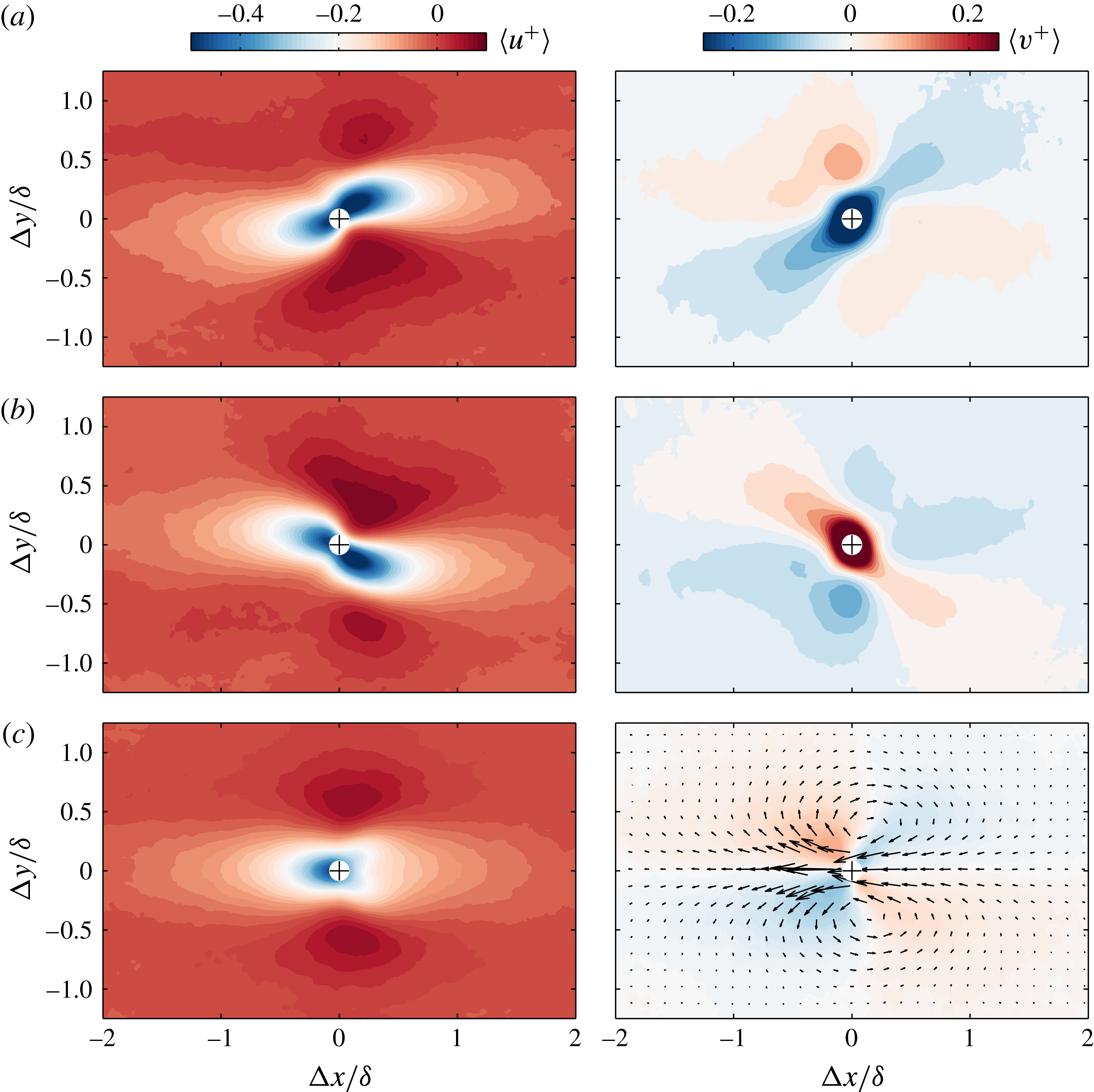
Figure 5. Colour contours of streamwise (
 $u$
) and spanwise (
$u$
) and spanwise (
 $v$
) velocity fluctuations conditioned for (a) only when
$v$
) velocity fluctuations conditioned for (a) only when
 $v<-\unicode[STIX]{x1D70E}_{v}$
, (b) only when
$v<-\unicode[STIX]{x1D70E}_{v}$
, (b) only when
 $v>\unicode[STIX]{x1D70E}_{v}$
and (c)
$v>\unicode[STIX]{x1D70E}_{v}$
and (c)
 $v>\unicode[STIX]{x1D70E}_{v}$
or
$v>\unicode[STIX]{x1D70E}_{v}$
or
 $v<-\unicode[STIX]{x1D70E}_{v}$
. Results are presented at
$v<-\unicode[STIX]{x1D70E}_{v}$
. Results are presented at
 $z\approx \unicode[STIX]{x1D6FF}$
and the arrows in (c) show the corresponding conditionally averaged two-component velocity field. The
$z\approx \unicode[STIX]{x1D6FF}$
and the arrows in (c) show the corresponding conditionally averaged two-component velocity field. The
 $+$
symbols correspond to the centroid of each detected region.
$+$
symbols correspond to the centroid of each detected region.
So far, we have examined the general nature of the two-point correlation functions based on the sign of
 $v$
, revealing a degree of preferential orientation which appears to have spatial extent of the order of the boundary layer thickness. Next, we examine conditionally averaged statistical properties in the near vicinity of these instantaneous features. To perform this, a frame of reference attached to the centroid of regions of strong
$v$
, revealing a degree of preferential orientation which appears to have spatial extent of the order of the boundary layer thickness. Next, we examine conditionally averaged statistical properties in the near vicinity of these instantaneous features. To perform this, a frame of reference attached to the centroid of regions of strong
 $u$
or
$u$
or
 $v$
fluctuations is employed as the conditioning point (i.e. the location at which
$v$
fluctuations is employed as the conditioning point (i.e. the location at which
 $\unicode[STIX]{x0394}x,\unicode[STIX]{x0394}y=0$
). Specifically, for a fixed wall-normal location, conditionally averaged flow fields are computed for coherent regions of
$\unicode[STIX]{x0394}x,\unicode[STIX]{x0394}y=0$
). Specifically, for a fixed wall-normal location, conditionally averaged flow fields are computed for coherent regions of
 $v$
in excess of one standard deviation of the spanwise turbulence intensity (
$v$
in excess of one standard deviation of the spanwise turbulence intensity (
 $\unicode[STIX]{x1D70E}_{v}$
). We note in the present work that as the databases are captured on wall-parallel planes of constant
$\unicode[STIX]{x1D70E}_{v}$
). We note in the present work that as the databases are captured on wall-parallel planes of constant
 $z/\unicode[STIX]{x1D6FF}$
, a single threshold can be applied across the entire spatial extent. Further, to omit small islands of low- and high-velocity fluctuations that might be associated with noise in the measured velocity fields, an area threshold equivalent to the Taylor microscale squared (
$z/\unicode[STIX]{x1D6FF}$
, a single threshold can be applied across the entire spatial extent. Further, to omit small islands of low- and high-velocity fluctuations that might be associated with noise in the measured velocity fields, an area threshold equivalent to the Taylor microscale squared (
 $\unicode[STIX]{x1D706}_{T}^{2}$
) is employed.
$\unicode[STIX]{x1D706}_{T}^{2}$
) is employed.
Figure 5(a,b) presents the velocity fluctuation signature conditioned for strong negatively and positively signed
 $v$
(in excess of
$v$
(in excess of
 $\pm \unicode[STIX]{x1D70E}_{v}$
) respectively at
$\pm \unicode[STIX]{x1D70E}_{v}$
) respectively at
 $z\approx \unicode[STIX]{x1D6FF}$
. From the results, it is immediately evident that
$z\approx \unicode[STIX]{x1D6FF}$
. From the results, it is immediately evident that
 $\langle v\rangle$
is counter-oriented dependent on its sign, and appears to have a spatial extent of
$\langle v\rangle$
is counter-oriented dependent on its sign, and appears to have a spatial extent of
 $1$
–
$1$
–
 $2\unicode[STIX]{x1D6FF}$
along its principal axis at least at the edge of the layer. The results also show that
$2\unicode[STIX]{x1D6FF}$
along its principal axis at least at the edge of the layer. The results also show that
 $\langle u\rangle$
appears to exhibit a comparable degree of preferential orientation based on the sign of
$\langle u\rangle$
appears to exhibit a comparable degree of preferential orientation based on the sign of
 $v$
. We note that the degree of preferential orientation in
$v$
. We note that the degree of preferential orientation in
 $u$
from the computed conditional statistics is more pronounced than is evident from the two-point correlation,
$u$
from the computed conditional statistics is more pronounced than is evident from the two-point correlation,
 $R_{uu}$
, conditioned on the sign of
$R_{uu}$
, conditioned on the sign of
 $v$
(see figure 4), which is caused by conditioning on only the strongest
$v$
(see figure 4), which is caused by conditioning on only the strongest
 $v$
regions in figure 5. Finally, figure 5(c) presents
$v$
regions in figure 5. Finally, figure 5(c) presents
 $\langle u\rangle$
and
$\langle u\rangle$
and
 $\langle v\rangle$
if one was to include both strong positive and negative signed
$\langle v\rangle$
if one was to include both strong positive and negative signed
 $v$
regions. Since conditioning on strong velocity fluctuations near the edge of the boundary layer (
$v$
regions. Since conditioning on strong velocity fluctuations near the edge of the boundary layer (
 $z\approx \unicode[STIX]{x1D6FF}$
) is analogous to conditioning on low-speed regions of
$z\approx \unicode[STIX]{x1D6FF}$
) is analogous to conditioning on low-speed regions of
 $u$
, we observe qualitatively comparable results. More specifically,
$u$
, we observe qualitatively comparable results. More specifically,
 $\langle u\rangle$
exhibits a low-speed region flanked by high-speed regions, and
$\langle u\rangle$
exhibits a low-speed region flanked by high-speed regions, and
 $\langle v\rangle$
exhibits the signature of a counter-rotating vortex pair on an
$\langle v\rangle$
exhibits the signature of a counter-rotating vortex pair on an
 $xy$
plane (vectors are plotted on figure 5(c) to demonstrate this arrangement). These signatures are characteristic of an inclined hairpin-like structure/eddy (see Tomkins & Adrian Reference Tomkins and Adrian2003; Adrian Reference Adrian2007; Elsinga et al.
Reference Elsinga, Adrian, Van Oudheusden and Scarano2010, and others), which has been reported to be present instantaneously in turbulent boundary layers. In § 6, we test whether such a prescribed set of eddies can reproduce the behaviour in the
$xy$
plane (vectors are plotted on figure 5(c) to demonstrate this arrangement). These signatures are characteristic of an inclined hairpin-like structure/eddy (see Tomkins & Adrian Reference Tomkins and Adrian2003; Adrian Reference Adrian2007; Elsinga et al.
Reference Elsinga, Adrian, Van Oudheusden and Scarano2010, and others), which has been reported to be present instantaneously in turbulent boundary layers. In § 6, we test whether such a prescribed set of eddies can reproduce the behaviour in the
 $v$
coherence observed in the experiments.
$v$
coherence observed in the experiments.
3.2 Distribution of orientation
To reaffirm and characterise these oblique features instantaneously, we quantify the distribution of their orientation. To perform this, the spanwise velocity fluctuations,
 $v$
, are first deconstructed into regions that are higher and lower than one standard deviation,
$v$
, are first deconstructed into regions that are higher and lower than one standard deviation,
 $\unicode[STIX]{x1D70E}_{v}$
. Binary representations are then computed for strong positive and negative
$\unicode[STIX]{x1D70E}_{v}$
. Binary representations are then computed for strong positive and negative
 $v$
following
$v$
following
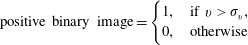 $$\begin{eqnarray}\displaystyle \text{positive binary image}=\left\{\begin{array}{@{}ll@{}}1,\quad & \text{if }v>\unicode[STIX]{x1D70E}_{v},\\ 0,\quad & \text{otherwise}\end{array}\right. & & \displaystyle\end{eqnarray}$$
and
 $$\begin{eqnarray}\displaystyle \text{negative binary image}=\left\{\begin{array}{@{}ll@{}}1,\quad & \text{if }v<-\unicode[STIX]{x1D70E}_{v},\\ 0,\quad & \text{otherwise}\end{array}\right. & & \displaystyle\end{eqnarray}$$
respectively. A representative example of a binary image computed for strong negative
 $v$
regions (3.2) is shown in figure 6. To extract the orientation of the detected features (black regions), we follow a principal component analysis, where a set of orthonormal vectors are computed that have the maximum variance along each direction under the constraint that the vectors are orthogonal to each other (a complete discussion can be found in Jolliffe (Reference Jolliffe1986)). This process is analogous to fitting an ellipse to each feature (solid red lines in figure 6), where the major and minor axes of each ellipse represent the principal components. Next, the angle between the major axis (red dashed line) and the flow direction,
$v$
regions (3.2) is shown in figure 6. To extract the orientation of the detected features (black regions), we follow a principal component analysis, where a set of orthonormal vectors are computed that have the maximum variance along each direction under the constraint that the vectors are orthogonal to each other (a complete discussion can be found in Jolliffe (Reference Jolliffe1986)). This process is analogous to fitting an ellipse to each feature (solid red lines in figure 6), where the major and minor axes of each ellipse represent the principal components. Next, the angle between the major axis (red dashed line) and the flow direction,
 $\unicode[STIX]{x1D703}$
, quantifies its orientation, as illustrated in figure 6(b).
$\unicode[STIX]{x1D703}$
, quantifies its orientation, as illustrated in figure 6(b).
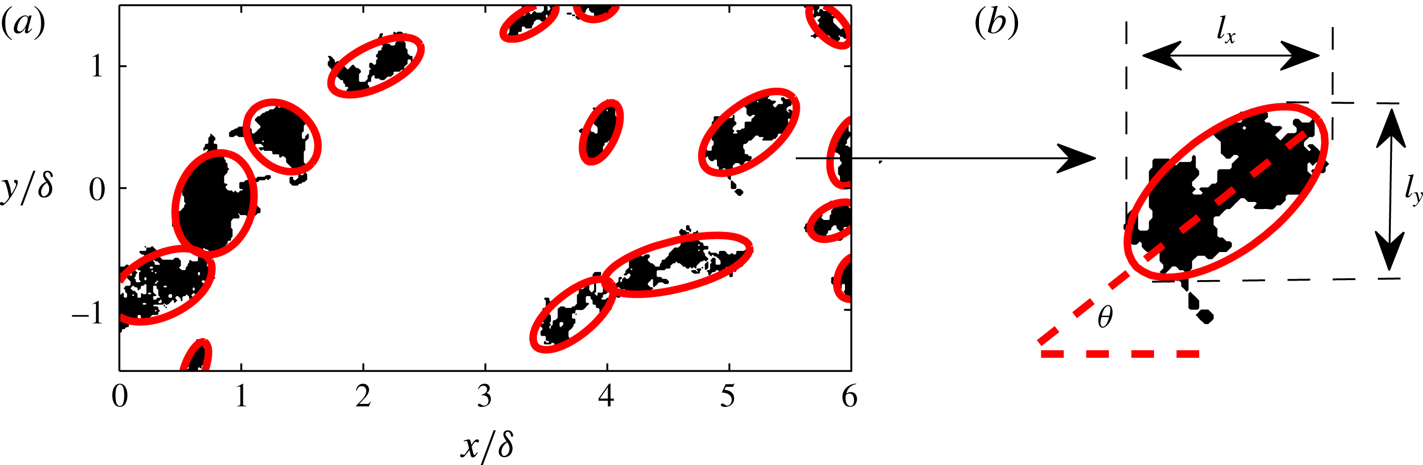
Figure 6. (a) Binary representation of coherent regions of
 $v$
satisfying
$v$
satisfying
 $v<-\unicode[STIX]{x1D70E}_{v}$
at
$v<-\unicode[STIX]{x1D70E}_{v}$
at
 $z\approx \unicode[STIX]{x1D6FF}$
. The red solid lines correspond to fitted ellipses in each region. (b) Schematic illustrating how the principal component analysis is employed to compute the orientation,
$z\approx \unicode[STIX]{x1D6FF}$
. The red solid lines correspond to fitted ellipses in each region. (b) Schematic illustrating how the principal component analysis is employed to compute the orientation,
 $\unicode[STIX]{x1D703}$
, of one region in (a). Here,
$\unicode[STIX]{x1D703}$
, of one region in (a). Here,
 $l_{x}$
and
$l_{x}$
and
 $l_{y}$
correspond to the streamwise and spanwise extent of each region respectively.
$l_{y}$
correspond to the streamwise and spanwise extent of each region respectively.
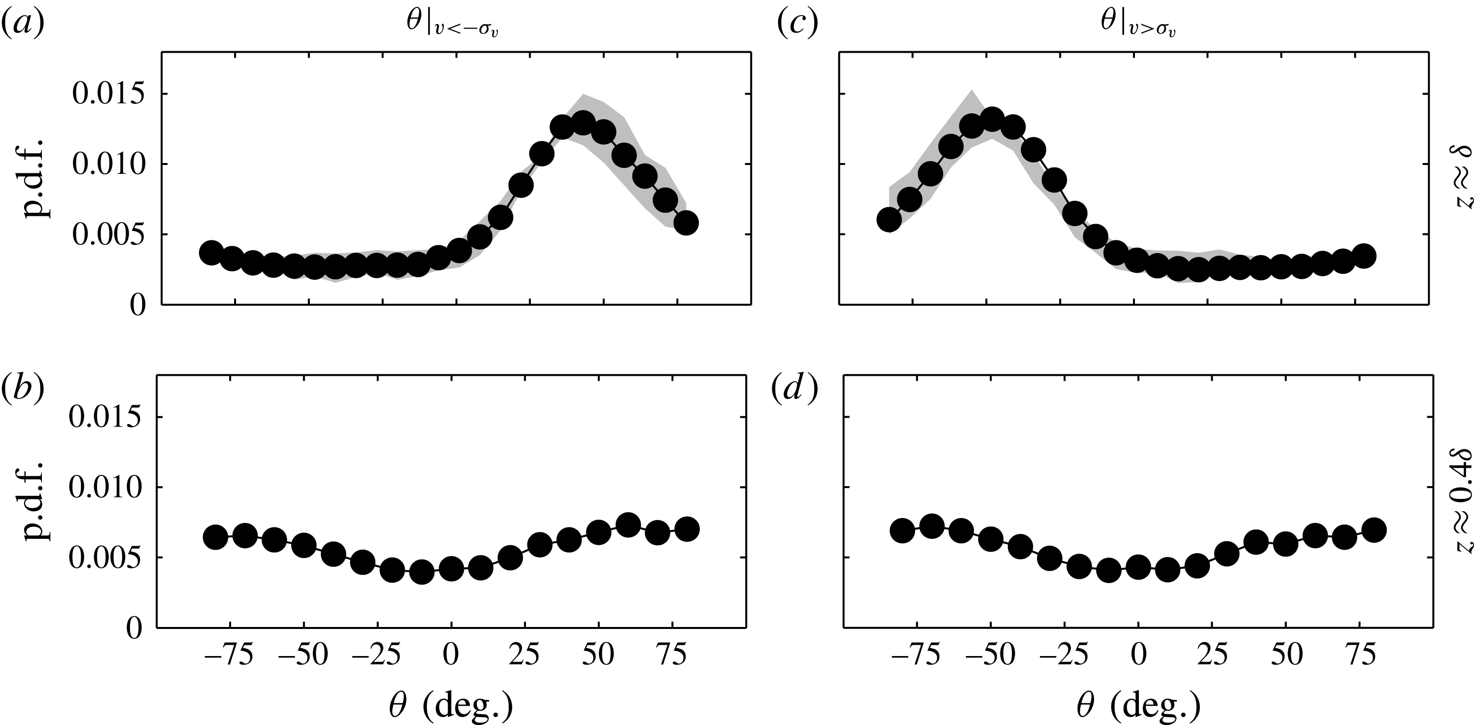
Figure 7. The p.d.f.s of the orientation,
 $\unicode[STIX]{x1D703}$
, of coherent regions of
$\unicode[STIX]{x1D703}$
, of coherent regions of
 $v$
conditioned for
$v$
conditioned for
 $v<-\unicode[STIX]{x1D70E}_{v}$
(a,b) and
$v<-\unicode[STIX]{x1D70E}_{v}$
(a,b) and
 $v>\unicode[STIX]{x1D70E}_{v}$
(c,d) at different wall-normal locations: (a,c)
$v>\unicode[STIX]{x1D70E}_{v}$
(c,d) at different wall-normal locations: (a,c)
 $z\approx \unicode[STIX]{x1D6FF}$
and (b,d)
$z\approx \unicode[STIX]{x1D6FF}$
and (b,d)
 $z\approx 0.4\unicode[STIX]{x1D6FF}$
. The shaded regions in (a,c) show the sensitivity to doubling or halving the threshold for
$z\approx 0.4\unicode[STIX]{x1D6FF}$
. The shaded regions in (a,c) show the sensitivity to doubling or halving the threshold for
 $v$
.
$v$
.
Figure 7 presents the probability density functions (p.d.f.s) of the orientation,
 $\unicode[STIX]{x1D703}$
, of all detected coherent regions of
$\unicode[STIX]{x1D703}$
, of all detected coherent regions of
 $v$
at the edge of the boundary layer (
$v$
at the edge of the boundary layer (
 $z\approx \unicode[STIX]{x1D6FF}$
). It should be noted that coherent regions that cross the edge of the FOV are excluded from the p.d.f. as their true spatial extent is not captured. Further, each p.d.f. is constructed with approximately
$z\approx \unicode[STIX]{x1D6FF}$
). It should be noted that coherent regions that cross the edge of the FOV are excluded from the p.d.f. as their true spatial extent is not captured. Further, each p.d.f. is constructed with approximately
 $10^{4}$
detected ensembles; consequently, only a negligible difference is observed by halving the number of ensembles. Figures 7(a,b) and 7(c,d) correspond to strong negative (
$10^{4}$
detected ensembles; consequently, only a negligible difference is observed by halving the number of ensembles. Figures 7(a,b) and 7(c,d) correspond to strong negative (
 $v<-\unicode[STIX]{x1D70E}_{v}$
) and positive (
$v<-\unicode[STIX]{x1D70E}_{v}$
) and positive (
 $v>\unicode[STIX]{x1D70E}_{v}$
) regions respectively. The results show a strong likelihood at
$v>\unicode[STIX]{x1D70E}_{v}$
) regions respectively. The results show a strong likelihood at
 $\unicode[STIX]{x1D703}\approx \pm 45^{\circ }$
, depending on the sign of
$\unicode[STIX]{x1D703}\approx \pm 45^{\circ }$
, depending on the sign of
 $v$
. These observations suggest that the
$v$
. These observations suggest that the
 $v$
coherence at the edge of the boundary layer throughout its existence is seemingly preferentially angled at
$v$
coherence at the edge of the boundary layer throughout its existence is seemingly preferentially angled at
 $\pm 45^{\circ }$
to the direction of the flow, rather than varying over a wide range of
$\pm 45^{\circ }$
to the direction of the flow, rather than varying over a wide range of
 $\unicode[STIX]{x1D703}$
. The robustness of this behaviour to the chosen threshold is quantified by the shaded regions in figure 7(a,c), which correspond to results computed by either halving or doubling the threshold used (i.e.
$\unicode[STIX]{x1D703}$
. The robustness of this behaviour to the chosen threshold is quantified by the shaded regions in figure 7(a,c), which correspond to results computed by either halving or doubling the threshold used (i.e.
 $\pm 0.5\unicode[STIX]{x1D70E}_{v}$
and
$\pm 0.5\unicode[STIX]{x1D70E}_{v}$
and
 $\pm 2\unicode[STIX]{x1D70E}_{v}$
). We note that a subtle asymmetry for
$\pm 2\unicode[STIX]{x1D70E}_{v}$
). We note that a subtle asymmetry for
 $\unicode[STIX]{x1D703}$
is present between
$\unicode[STIX]{x1D703}$
is present between
 $v<-\unicode[STIX]{x1D70E}_{v}$
and positive
$v<-\unicode[STIX]{x1D70E}_{v}$
and positive
 $v>\unicode[STIX]{x1D70E}_{v}$
regions (see figure 7), which might be associated with the criteria to compute
$v>\unicode[STIX]{x1D70E}_{v}$
regions (see figure 7), which might be associated with the criteria to compute
 $\unicode[STIX]{x1D703}$
and other experimental uncertainties (alignment of laser sheet/calibration). In any case, a strong preferential orientation at
$\unicode[STIX]{x1D703}$
and other experimental uncertainties (alignment of laser sheet/calibration). In any case, a strong preferential orientation at
 ${\approx}\pm 45^{\circ }$
to the direction of the flow is clearly present based on the sign of
${\approx}\pm 45^{\circ }$
to the direction of the flow is clearly present based on the sign of
 $v$
. Further, our results also show that the oblique orientation is more pronounced if one only includes regions that have lengths of
$v$
. Further, our results also show that the oblique orientation is more pronounced if one only includes regions that have lengths of
 $O(\unicode[STIX]{x1D6FF})$
(not reproduced here). This highlights the fact that the underpinning structures of this behaviour are likely to be associated with the large-scale motions prevalent in the boundary layer (Hutchins & Marusic Reference Hutchins and Marusic2007).
$O(\unicode[STIX]{x1D6FF})$
(not reproduced here). This highlights the fact that the underpinning structures of this behaviour are likely to be associated with the large-scale motions prevalent in the boundary layer (Hutchins & Marusic Reference Hutchins and Marusic2007).
Figure 7(b,d) reproduces the p.d.f. of
 $\unicode[STIX]{x1D703}$
closer to the wall at
$\unicode[STIX]{x1D703}$
closer to the wall at
 $z\approx 0.4\unicode[STIX]{x1D6FF}$
, where no strong preferential orientation is observed instantaneously based only on the sign of
$z\approx 0.4\unicode[STIX]{x1D6FF}$
, where no strong preferential orientation is observed instantaneously based only on the sign of
 $v$
when compared with the edge of the boundary layer. The results exhibit a subtle preference in alignment at
$v$
when compared with the edge of the boundary layer. The results exhibit a subtle preference in alignment at
 $|\unicode[STIX]{x1D703}|>\pm 50^{\circ }$
at
$|\unicode[STIX]{x1D703}|>\pm 50^{\circ }$
at
 $z\approx 0.4\unicode[STIX]{x1D6FF}$
. This observation is probably a consequence of the
$z\approx 0.4\unicode[STIX]{x1D6FF}$
. This observation is probably a consequence of the
 $v$
coherence on average exhibiting a slightly longer spanwise (
$v$
coherence on average exhibiting a slightly longer spanwise (
 $y$
) extent than the streamwise direction on a
$y$
) extent than the streamwise direction on a
 $xy$
plane (see the contours of
$xy$
plane (see the contours of
 $R_{vv}$
at 0.2 and 0.4 presented in figure 3
b–i); consequently, there is an increased likelihood that the major axis of the fitted ellipses used to compute
$R_{vv}$
at 0.2 and 0.4 presented in figure 3
b–i); consequently, there is an increased likelihood that the major axis of the fitted ellipses used to compute
 $\unicode[STIX]{x1D703}$
exceeds
$\unicode[STIX]{x1D703}$
exceeds
 $\pm 45^{\circ }$
to the direction of the flow. Furthermore, the boundary layer is composed of both small and large scales closer to the wall, unlike at
$\pm 45^{\circ }$
to the direction of the flow. Furthermore, the boundary layer is composed of both small and large scales closer to the wall, unlike at
 $z\approx \unicode[STIX]{x1D6FF}$
, where
$z\approx \unicode[STIX]{x1D6FF}$
, where
 $\unicode[STIX]{x1D6FF}$
-scaled features dominate (see figure 1
b). Therefore, to ensure that the behaviour reported for
$\unicode[STIX]{x1D6FF}$
-scaled features dominate (see figure 1
b). Therefore, to ensure that the behaviour reported for
 $\unicode[STIX]{x1D703}$
is associated with the large-scale spanwise coherence, a p.d.f. of
$\unicode[STIX]{x1D703}$
is associated with the large-scale spanwise coherence, a p.d.f. of
 $\unicode[STIX]{x1D703}$
is recomputed from velocity fields that are filtered to only include scales larger than
$\unicode[STIX]{x1D703}$
is recomputed from velocity fields that are filtered to only include scales larger than
 $\unicode[STIX]{x1D6FF}$
. The results (not reproduced here) show negligible difference from those presented in figure 7(b,d). In § 4, we revisit the statistical properties of the
$\unicode[STIX]{x1D6FF}$
. The results (not reproduced here) show negligible difference from those presented in figure 7(b,d). In § 4, we revisit the statistical properties of the
 $v$
coherence in order to further examine these features in the logarithmic region.
$v$
coherence in order to further examine these features in the logarithmic region.
3.3 The spatial extent of the oblique features
Qualitatively, through visual inspections of the
 $xy$
velocity fields, the diagonal-like pattern appears to extend throughout the full spatial domain (see figure 1), although on average it appears to be uncorrelated beyond
$xy$
velocity fields, the diagonal-like pattern appears to extend throughout the full spatial domain (see figure 1), although on average it appears to be uncorrelated beyond
 $1$
–
$1$
–
 $2\unicode[STIX]{x1D6FF}$
(see figure 3). In fact, through visual inspections in numerical simulations, Sillero et al. (Reference Sillero, Jiménez and Moser2014) observed the obliqueness in
$2\unicode[STIX]{x1D6FF}$
(see figure 3). In fact, through visual inspections in numerical simulations, Sillero et al. (Reference Sillero, Jiménez and Moser2014) observed the obliqueness in
 $v$
coherence to be visible across a spanwise domain of
$v$
coherence to be visible across a spanwise domain of
 $({\sim}10\unicode[STIX]{x1D6FF})$
, albeit qualitatively. Similar patterns have also been reported over large spatial extents in supersonic flow (Elsinga et al.
Reference Elsinga, Adrian, Van Oudheusden and Scarano2010), where the signature of large-scale hairpin-like structures is observed in the autocorrelation of the wall-normal swirl. Works in other wall-bounded flows, albeit in low
$({\sim}10\unicode[STIX]{x1D6FF})$
, albeit qualitatively. Similar patterns have also been reported over large spatial extents in supersonic flow (Elsinga et al.
Reference Elsinga, Adrian, Van Oudheusden and Scarano2010), where the signature of large-scale hairpin-like structures is observed in the autocorrelation of the wall-normal swirl. Works in other wall-bounded flows, albeit in low
 $Re$
/transitionally turbulent flows (plane Couette/Poiseuille flow Duguet & Schlatter Reference Duguet and Schlatter2013 and spiral turbulence/Taylor–Couette flow Coles Reference Coles1965; Van Atta Reference Van Atta1966), have also observed similar oblique patterns in turbulent patches. These works reported that the large-scale flow distorts the shape of turbulent patches and is responsible for their oblique growth (leading to oblique turbulent stripes). We note that an examination of the growth of these oblique features would necessitate temporally resolved databases, which are unavailable in the present work. Instead, in the subsequent discussion, using the large instantaneous snapshots, we aim to quantify the spatial extent and any alignment between multiple oblique features in the
$Re$
/transitionally turbulent flows (plane Couette/Poiseuille flow Duguet & Schlatter Reference Duguet and Schlatter2013 and spiral turbulence/Taylor–Couette flow Coles Reference Coles1965; Van Atta Reference Van Atta1966), have also observed similar oblique patterns in turbulent patches. These works reported that the large-scale flow distorts the shape of turbulent patches and is responsible for their oblique growth (leading to oblique turbulent stripes). We note that an examination of the growth of these oblique features would necessitate temporally resolved databases, which are unavailable in the present work. Instead, in the subsequent discussion, using the large instantaneous snapshots, we aim to quantify the spatial extent and any alignment between multiple oblique features in the
 $v$
coherence. Further, in § 6, we examine whether a collection of large-scale self-similar hairpin-like structures (following the attached eddy model) is able to reproduce the obliqueness in the
$v$
coherence. Further, in § 6, we examine whether a collection of large-scale self-similar hairpin-like structures (following the attached eddy model) is able to reproduce the obliqueness in the
 $v$
coherence.
$v$
coherence.
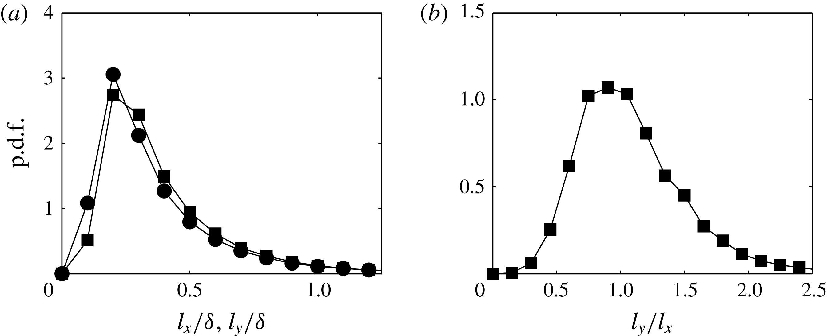
Figure 8. (a) The p.d.f.s of the streamwise (
 $l_{x}$
) and spanwise (
$l_{x}$
) and spanwise (
 $l_{y}$
) extents for coherent regions of
$l_{y}$
) extents for coherent regions of
 $v$
satisfying
$v$
satisfying
 $v<-\unicode[STIX]{x1D70E}_{v}$
at
$v<-\unicode[STIX]{x1D70E}_{v}$
at
 $z\approx \unicode[STIX]{x1D6FF}$
. The ● and ▪ symbols in (a) correspond to
$z\approx \unicode[STIX]{x1D6FF}$
. The ● and ▪ symbols in (a) correspond to
 $l_{x}$
and
$l_{x}$
and
 $l_{y}$
respectively. (b) The ratio
$l_{y}$
respectively. (b) The ratio
 $l_{y}/l_{x}$
.
$l_{y}/l_{x}$
.
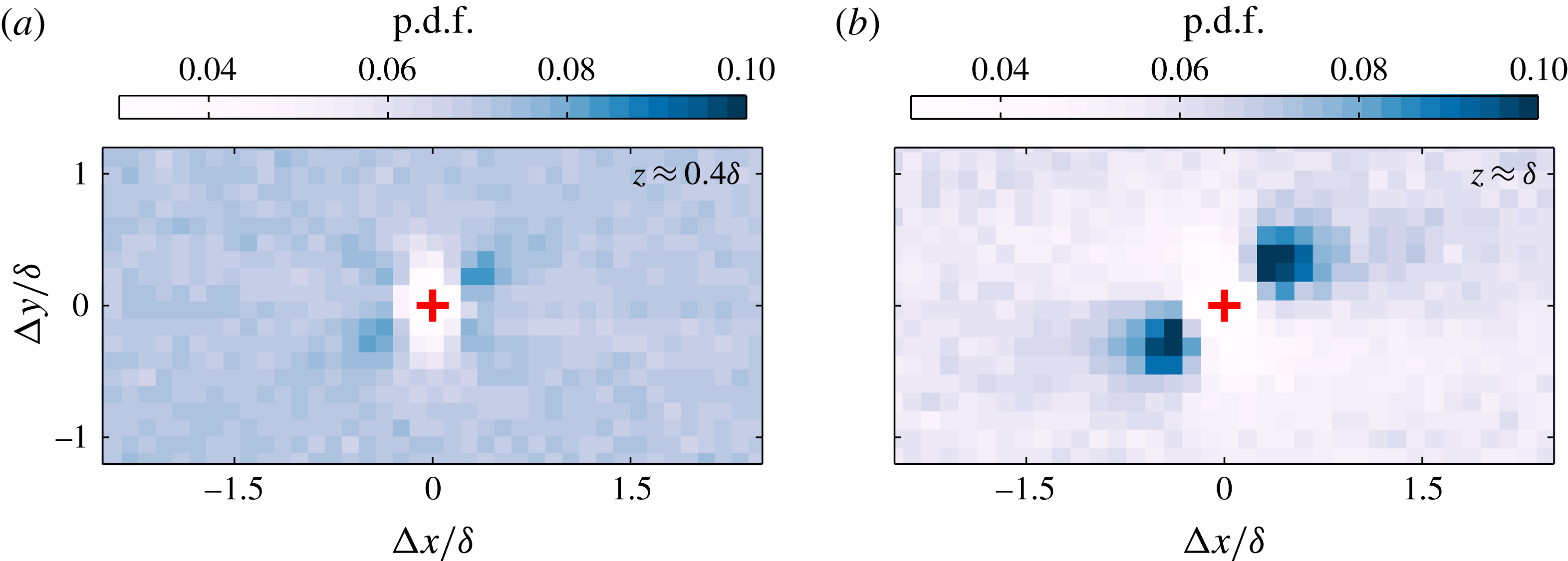
Figure 9. The p.d.f.s of centroid locations for coherent regions of
 $v$
satisfying
$v$
satisfying
 $v<-\unicode[STIX]{x1D70E}_{v}$
: (a)
$v<-\unicode[STIX]{x1D70E}_{v}$
: (a)
 $z\approx 0.4\unicode[STIX]{x1D6FF}$
and (b)
$z\approx 0.4\unicode[STIX]{x1D6FF}$
and (b)
 $z\approx \unicode[STIX]{x1D6FF}$
.
$z\approx \unicode[STIX]{x1D6FF}$
.
To this end, the streamwise (
 $l_{x}$
) and spanwise (
$l_{x}$
) and spanwise (
 $l_{y}$
) lengths (illustrated in figure 6
b) of coherent regions of
$l_{y}$
) lengths (illustrated in figure 6
b) of coherent regions of
 $v$
are extracted from a binary representation above a certain threshold, here chosen to be
$v$
are extracted from a binary representation above a certain threshold, here chosen to be
 $\pm \unicode[STIX]{x1D70E}_{v}$
following the preceding discussion. The p.d.f.s of
$\pm \unicode[STIX]{x1D70E}_{v}$
following the preceding discussion. The p.d.f.s of
 $l_{x}$
and
$l_{x}$
and
 $l_{y}$
are plotted in figure 8(a), showing good agreement between the two distributions, hinting that the structures appear to mostly have a ratio of one between their streamwise and spanwise lengths. To verify this observation, figure 8(b) presents the ratio
$l_{y}$
are plotted in figure 8(a), showing good agreement between the two distributions, hinting that the structures appear to mostly have a ratio of one between their streamwise and spanwise lengths. To verify this observation, figure 8(b) presents the ratio
 $l_{y}/l_{x}$
, which shows the expected peak at one. Further, these results also concur with our previous findings that coherent regions of spanwise velocity are oriented at
$l_{y}/l_{x}$
, which shows the expected peak at one. Further, these results also concur with our previous findings that coherent regions of spanwise velocity are oriented at
 $\pm 45^{\circ }$
(i.e
$\pm 45^{\circ }$
(i.e
 $l_{x}\approxeq l_{y}$
) to the direction of the flow at the edge of the boundary layer. The p.d.f.s of
$l_{x}\approxeq l_{y}$
) to the direction of the flow at the edge of the boundary layer. The p.d.f.s of
 $l_{x}$
and
$l_{x}$
and
 $l_{y}$
in figure 8(a) also show that the spatial extent of each binary region extends up to
$l_{y}$
in figure 8(a) also show that the spatial extent of each binary region extends up to
 ${\sim}\unicode[STIX]{x1D6FF}$
. However, this quantitative measure is dependent on the chosen threshold, and therefore should be taken with caution. Additionally, since these features appear to visually span much longer lengths (see figure 1), in the subsequent discussion, we inspect any preferential alignment between multiple oblique features along counter-oriented diagonals.
${\sim}\unicode[STIX]{x1D6FF}$
. However, this quantitative measure is dependent on the chosen threshold, and therefore should be taken with caution. Additionally, since these features appear to visually span much longer lengths (see figure 1), in the subsequent discussion, we inspect any preferential alignment between multiple oblique features along counter-oriented diagonals.
Accordingly, instead of conditioning the velocity signal, we examine the centroid locations of neighbouring coherent regions of
 $v$
and construct a p.d.f. of their locations. Such a diagnostic is also less susceptible to any change in threshold, as a higher (or lower) threshold would simply lead to more (or less) centroids being found still located in the near vicinity of the original centroid locations. The results are presented in figure 9, which shows colour contours corresponding to the p.d.f.s of the aforementioned neighbouring centroid locations. Here, any preferential arrangement of these centroids (coherent regions) will be reflected by a non-uniform distribution. The p.d.f. for
$v$
and construct a p.d.f. of their locations. Such a diagnostic is also less susceptible to any change in threshold, as a higher (or lower) threshold would simply lead to more (or less) centroids being found still located in the near vicinity of the original centroid locations. The results are presented in figure 9, which shows colour contours corresponding to the p.d.f.s of the aforementioned neighbouring centroid locations. Here, any preferential arrangement of these centroids (coherent regions) will be reflected by a non-uniform distribution. The p.d.f. for
 $z\approx 0.4\unicode[STIX]{x1D6FF}$
shows no significant preferential organisation of strong negative
$z\approx 0.4\unicode[STIX]{x1D6FF}$
shows no significant preferential organisation of strong negative
 $v$
regions, while in the far wake (
$v$
regions, while in the far wake (
 $z\approx \unicode[STIX]{x1D6FF}$
), they appear to reside preferentially aligned at
$z\approx \unicode[STIX]{x1D6FF}$
), they appear to reside preferentially aligned at
 $+45^{\circ }$
(darker shaded regions) with an extent of
$+45^{\circ }$
(darker shaded regions) with an extent of
 $1$
–
$1$
–
 $2\unicode[STIX]{x1D6FF}$
about the conditioning point. This quantitative estimate provides us with a measure of the size of the underlying structures that lead to the preferentially aligned
$2\unicode[STIX]{x1D6FF}$
about the conditioning point. This quantitative estimate provides us with a measure of the size of the underlying structures that lead to the preferentially aligned
 $v$
structures. It should be noted that in the near vicinity of
$v$
structures. It should be noted that in the near vicinity of
 $\unicode[STIX]{x1D6E5}x,\unicode[STIX]{x1D6E5}y=0$
, due to the spatial extent of the region being conditioned, other centroids are not detected (which is manifested as a lower magnitude on the p.d.f.). Nevertheless, our results confirm that although these features appear to visually span much longer lengths (see figure 1), their placement is uncorrelated beyond
$\unicode[STIX]{x1D6E5}x,\unicode[STIX]{x1D6E5}y=0$
, due to the spatial extent of the region being conditioned, other centroids are not detected (which is manifested as a lower magnitude on the p.d.f.). Nevertheless, our results confirm that although these features appear to visually span much longer lengths (see figure 1), their placement is uncorrelated beyond
 $1$
–
$1$
–
 $2\unicode[STIX]{x1D6FF}$
and is limited in spatial extent to only the order of the large-scale motions (LSMs) in the flow. These findings are also supported by the correlation results presented in § 3.1, where
$2\unicode[STIX]{x1D6FF}$
and is limited in spatial extent to only the order of the large-scale motions (LSMs) in the flow. These findings are also supported by the correlation results presented in § 3.1, where
 $R_{vv}$
conditioned on
$R_{vv}$
conditioned on
 $v<0$
and
$v<0$
and
 $v>0$
is near zero beyond
$v>0$
is near zero beyond
 $2\unicode[STIX]{x1D6FF}$
. Elsinga et al. (Reference Elsinga, Adrian, Van Oudheusden and Scarano2010) also reported a streamwise–spanwise alignment of hairpin-like structures over comparable spatial extents, albeit using the swirling strength as a diagnostic and in a compressible turbulent boundary layer. We note, based on our observations, that the obliqueness in the
$2\unicode[STIX]{x1D6FF}$
. Elsinga et al. (Reference Elsinga, Adrian, Van Oudheusden and Scarano2010) also reported a streamwise–spanwise alignment of hairpin-like structures over comparable spatial extents, albeit using the swirling strength as a diagnostic and in a compressible turbulent boundary layer. We note, based on our observations, that the obliqueness in the
 $v$
coherence is of the order of the LSMs in the flow; therefore, we expect these features to persist in a similar form at higher
$v$
coherence is of the order of the LSMs in the flow; therefore, we expect these features to persist in a similar form at higher
 $Re$
(where the LSMs show very little
$Re$
(where the LSMs show very little
 $Re$
dependence for
$Re$
dependence for
 $z/\unicode[STIX]{x1D6FF}>0.5$
). However, high-
$z/\unicode[STIX]{x1D6FF}>0.5$
). However, high-
 $Re$
databases with comparable spatial extents would be necessary to confirm the presence of these features, which are unavailable in the present work.
$Re$
databases with comparable spatial extents would be necessary to confirm the presence of these features, which are unavailable in the present work.
4 Spanwise coherence in the logarithmic region
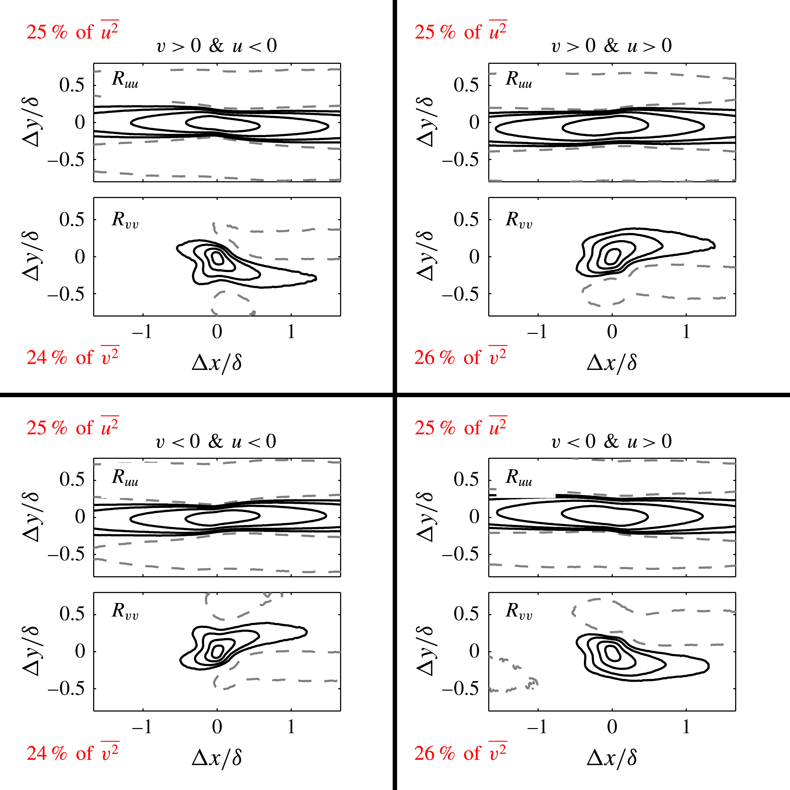
Figure 10. Wall-parallel slices of the correlation functions
 $R_{vv}$
and
$R_{vv}$
and
 $R_{uu}$
deconstructed into quadrants based on the signs of
$R_{uu}$
deconstructed into quadrants based on the signs of
 $u$
and
$u$
and
 $v$
. Results are presented in the logarithmic region (
$v$
. Results are presented in the logarithmic region (
 $z\approx 0.1\unicode[STIX]{x1D6FF}$
). The positive contours (solid lines) are 0.05, 0.1, 0.2 and 0.4 and the negative contours (dashed lines) are
$z\approx 0.1\unicode[STIX]{x1D6FF}$
). The positive contours (solid lines) are 0.05, 0.1, 0.2 and 0.4 and the negative contours (dashed lines) are
 $-$
0.02. The percentage contributions of each quadrant to the total turbulence intensity for
$-$
0.02. The percentage contributions of each quadrant to the total turbulence intensity for
 $u$
and
$u$
and
 $v$
are shown in red font.
$v$
are shown in red font.
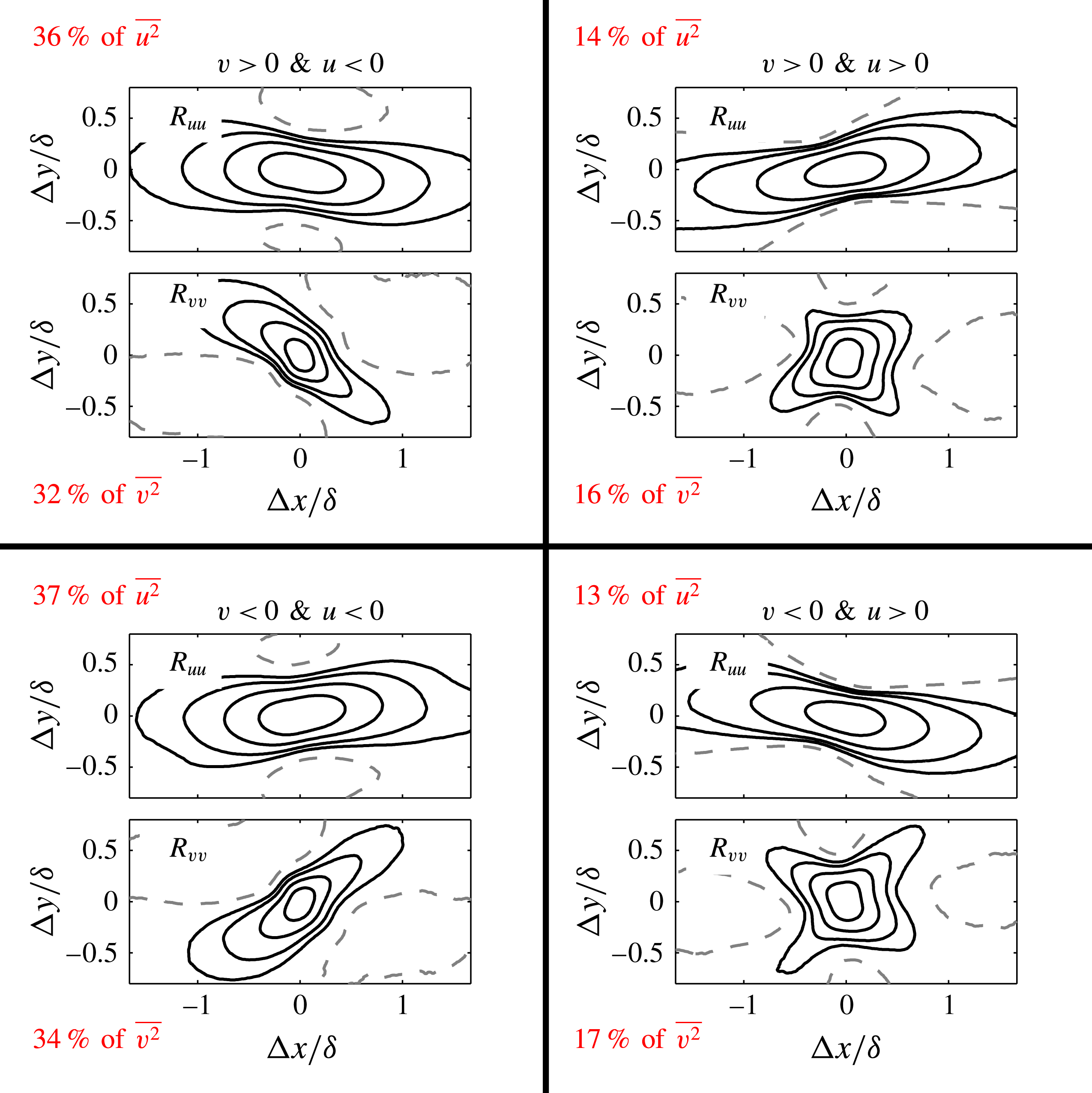
Figure 11. The autocorrelation functions presented in figure 10 reproduced at the edge of the boundary layer (
 $z\approx \unicode[STIX]{x1D6FF}$
).
$z\approx \unicode[STIX]{x1D6FF}$
).
So far, we have evidenced oblique features in the spanwise coherence at the top edge of a turbulent boundary layer based on the sign of
 $v$
(see figures 3 and 7). However, closer to the wall, simply considering only the sign of
$v$
(see figures 3 and 7). However, closer to the wall, simply considering only the sign of
 $v$
showed no clear evidence, despite the characteristically squarish shape of the two-point correlation function,
$v$
showed no clear evidence, despite the characteristically squarish shape of the two-point correlation function,
 $R_{vv}$
(see figure 3
c,f,i). To examine this further, figure 10 presents
$R_{vv}$
(see figure 3
c,f,i). To examine this further, figure 10 presents
 $R_{uu}$
and
$R_{uu}$
and
 $R_{vv}$
decomposed by the signs of both
$R_{vv}$
decomposed by the signs of both
 $u$
and
$u$
and
 $v$
in the logarithmic region (
$v$
in the logarithmic region (
 $z\approx 0.1\unicode[STIX]{x1D6FF}$
). We note that such a decomposition is analogous to the classical quadrant analysis usually reported between the streamwise and wall-normal velocity fluctuations,
$z\approx 0.1\unicode[STIX]{x1D6FF}$
). We note that such a decomposition is analogous to the classical quadrant analysis usually reported between the streamwise and wall-normal velocity fluctuations,
 $u$
and
$u$
and
 $w$
(Wallace, Eckelmann & Brodkey Reference Wallace, Eckelmann and Brodkey1972). Interestingly, when considering only one sign of
$w$
(Wallace, Eckelmann & Brodkey Reference Wallace, Eckelmann and Brodkey1972). Interestingly, when considering only one sign of
 $u$
(i.e. either low- or high-speed region), an oblique signature in
$u$
(i.e. either low- or high-speed region), an oblique signature in
 $R_{vv}$
is present, albeit at a shallower angle than at the edge of the boundary layer (see figure 10). It can also be noted that the
$R_{vv}$
is present, albeit at a shallower angle than at the edge of the boundary layer (see figure 10). It can also be noted that the
 $v$
coherence is counter-oriented between positive and negative
$v$
coherence is counter-oriented between positive and negative
 $u$
(compare ‘quadrants’ 1 and 2 for example); therefore, the low and high streamwise momentum is accompanied by counter-oriented positive (or negative)
$u$
(compare ‘quadrants’ 1 and 2 for example); therefore, the low and high streamwise momentum is accompanied by counter-oriented positive (or negative)
 $v$
regions. Moreover, the meandering behaviour of
$v$
regions. Moreover, the meandering behaviour of
 $u$
also appears statistically in
$u$
also appears statistically in
 $R_{uu}$
, following this quadrant conditioning. This observation suggests that the meandering of the
$R_{uu}$
, following this quadrant conditioning. This observation suggests that the meandering of the
 $u$
coherence reported previously (see Hutchins & Marusic Reference Hutchins and Marusic2007) is likely to be related to a more pronounced obliqueness of the spanwise coherence. We note that the lack of an oblique signature in the correlation functions based only on the sign of
$u$
coherence reported previously (see Hutchins & Marusic Reference Hutchins and Marusic2007) is likely to be related to a more pronounced obliqueness of the spanwise coherence. We note that the lack of an oblique signature in the correlation functions based only on the sign of
 $v$
in the logarithmic region (see figure 3 and also Sillero et al.
Reference Sillero, Jiménez and Moser2014) is due to the counter-oriented arrangement based on the sign of
$v$
in the logarithmic region (see figure 3 and also Sillero et al.
Reference Sillero, Jiménez and Moser2014) is due to the counter-oriented arrangement based on the sign of
 $u$
, combined with each quadrant (
$u$
, combined with each quadrant (
 $u>0$
and
$u>0$
and
 $u<0$
) contributing equally to the turbulence intensity (see the percentage contributions in figure 10 in red font).
$u<0$
) contributing equally to the turbulence intensity (see the percentage contributions in figure 10 in red font).
Figure 11 reproduces the same quadrant deconstruction based on the signs of
 $u$
and
$u$
and
 $v$
in the far-wake region at
$v$
in the far-wake region at
 $z\approx \unicode[STIX]{x1D6FF}$
. It should be noted that, at the edge of the boundary layer, only the negative
$z\approx \unicode[STIX]{x1D6FF}$
. It should be noted that, at the edge of the boundary layer, only the negative
 $u$
regions will tend to be in turbulent regions, while positive
$u$
regions will tend to be in turbulent regions, while positive
 $u$
regions are likely to be potential flow. This is reflected by the higher contributions to the turbulence intensity from quadrants 2 and 3 (where
$u$
regions are likely to be potential flow. This is reflected by the higher contributions to the turbulence intensity from quadrants 2 and 3 (where
 $u<0$
) to the turbulence intensity. As a consequence, at the edge of the boundary layer, the pronounced preferential orientation exhibited by low-streamwise-momentum events (
$u<0$
) to the turbulence intensity. As a consequence, at the edge of the boundary layer, the pronounced preferential orientation exhibited by low-streamwise-momentum events (
 $u<0$
) on
$u<0$
) on
 $R_{vv}$
is still evident when only conditioned on the sign of
$R_{vv}$
is still evident when only conditioned on the sign of
 $v$
(see § 3.1). The
$v$
(see § 3.1). The
 $R_{uu}$
plots appear to show strong opposing preferential orientation based on the signs of both
$R_{uu}$
plots appear to show strong opposing preferential orientation based on the signs of both
 $u$
and
$u$
and
 $v$
, albeit with a shorter streamwise extent compared with the logarithmic region (see figure 10). This observation is in agreement with the turbulent bulges of
$v$
, albeit with a shorter streamwise extent compared with the logarithmic region (see figure 10). This observation is in agreement with the turbulent bulges of
 $u$
that are observed in the wake region of a boundary layer, which have shorter streamwise extents than the streamwise elongated streaky patterns of
$u$
that are observed in the wake region of a boundary layer, which have shorter streamwise extents than the streamwise elongated streaky patterns of
 $u$
coherence reported in the logarithmic region (Hutchins & Marusic Reference Hutchins and Marusic2007). In short, our results support the fact that the clear obliqueness in the
$u$
coherence reported in the logarithmic region (Hutchins & Marusic Reference Hutchins and Marusic2007). In short, our results support the fact that the clear obliqueness in the
 $v$
coherence we observe at the edge of the boundary layer appears to be related to low-streamwise-momentum events, and their orientation is shown here to be consistent throughout the boundary layer even closer to the wall (logarithmic region).
$v$
coherence we observe at the edge of the boundary layer appears to be related to low-streamwise-momentum events, and their orientation is shown here to be consistent throughout the boundary layer even closer to the wall (logarithmic region).
5 Impact on the turbulent bulges and their interfaces
Encouraged by the fact that the
 $v$
coherence exhibits strong oblique behaviour, we suspect that the turbulent bulges (Robinson Reference Robinson1991) and the turbulent/non-turbulent interface (hereafter referred to as the TNTI) may also display a tendency to be impacted by this behaviour. In order to examine this further, we begin with a brief discussion on the detection of the TNTI, which has been spatially located using a number of techniques in the past. These include methods based on thresholds of vorticity (Bisset, Hunt & Rogers Reference Bisset, Hunt and Rogers2002; Mathew & Basu Reference Mathew and Basu2002; Jiménez et al.
Reference Jiménez, Hoyas, Simens and Mizuno2010), kinetic energy (de Silva et al.
Reference de Silva, Philip, Chauhan, Meneveau and Marusic2013; Chauhan, Philip & Marusic Reference Chauhan, Philip and Marusic2014), mean velocity (Anand, Boersma & Agrawal Reference Anand, Boersma and Agrawal2009) and velocity fluctuations (Heskestad Reference Heskestad1965). In the present study, the velocity fields are obtained from PIV experiments; therefore, we employ a kinetic energy threshold, which has been shown previously to be well-suited to locating the TNTI from PIV databases (see de Silva et al.
Reference de Silva, Philip, Chauhan, Meneveau and Marusic2013 and Chauhan et al.
Reference Chauhan, Philip and Marusic2014). In order to associate the non-turbulent outer region with zero kinetic energy, we compute the kinetic energy in a frame moving with the free stream, i.e. the defect kinetic energy, which is defined according to
$v$
coherence exhibits strong oblique behaviour, we suspect that the turbulent bulges (Robinson Reference Robinson1991) and the turbulent/non-turbulent interface (hereafter referred to as the TNTI) may also display a tendency to be impacted by this behaviour. In order to examine this further, we begin with a brief discussion on the detection of the TNTI, which has been spatially located using a number of techniques in the past. These include methods based on thresholds of vorticity (Bisset, Hunt & Rogers Reference Bisset, Hunt and Rogers2002; Mathew & Basu Reference Mathew and Basu2002; Jiménez et al.
Reference Jiménez, Hoyas, Simens and Mizuno2010), kinetic energy (de Silva et al.
Reference de Silva, Philip, Chauhan, Meneveau and Marusic2013; Chauhan, Philip & Marusic Reference Chauhan, Philip and Marusic2014), mean velocity (Anand, Boersma & Agrawal Reference Anand, Boersma and Agrawal2009) and velocity fluctuations (Heskestad Reference Heskestad1965). In the present study, the velocity fields are obtained from PIV experiments; therefore, we employ a kinetic energy threshold, which has been shown previously to be well-suited to locating the TNTI from PIV databases (see de Silva et al.
Reference de Silva, Philip, Chauhan, Meneveau and Marusic2013 and Chauhan et al.
Reference Chauhan, Philip and Marusic2014). In order to associate the non-turbulent outer region with zero kinetic energy, we compute the kinetic energy in a frame moving with the free stream, i.e. the defect kinetic energy, which is defined according to
 $$\begin{eqnarray}\displaystyle K={\textstyle \frac{1}{2}}[(\widetilde{U}-U_{\infty })^{2}+\widetilde{V}^{2}]. & & \displaystyle\end{eqnarray}$$
Figure 12 shows a sample PIV image and the interface determined based on the local defect kinetic energy
 $K$
, using a threshold of
$K$
, using a threshold of
 $K_{0}=10^{-3}((1/2)U_{\infty }^{2})$
. The appropriate threshold to be used depends on the flow, as well as on the level of free-stream (background) turbulence and measurement noise. Here, it is chosen such that the detected TNTI matches the appropriate intermittency between turbulent and non-turbulent regions for a given wall-normal location. We note that similar thresholds have also been employed by de Silva et al. (Reference de Silva, Philip, Chauhan, Meneveau and Marusic2013), Chauhan et al. (Reference Chauhan, Philip and Marusic2014) and Philip et al. (Reference Philip, Meneveau, de Silva and Marusic2014) to characterise various interface properties such as the fractal dimension, intermittency and conditional averages. We also note that the chosen threshold yields an interface that agrees well with the location that visually can be observed to separate the turbulent flow (the shaded region) from the non-turbulent flow (the unshaded region where
$K_{0}=10^{-3}((1/2)U_{\infty }^{2})$
. The appropriate threshold to be used depends on the flow, as well as on the level of free-stream (background) turbulence and measurement noise. Here, it is chosen such that the detected TNTI matches the appropriate intermittency between turbulent and non-turbulent regions for a given wall-normal location. We note that similar thresholds have also been employed by de Silva et al. (Reference de Silva, Philip, Chauhan, Meneveau and Marusic2013), Chauhan et al. (Reference Chauhan, Philip and Marusic2014) and Philip et al. (Reference Philip, Meneveau, de Silva and Marusic2014) to characterise various interface properties such as the fractal dimension, intermittency and conditional averages. We also note that the chosen threshold yields an interface that agrees well with the location that visually can be observed to separate the turbulent flow (the shaded region) from the non-turbulent flow (the unshaded region where
 $K\approx 0$
) in figure 12.
$K\approx 0$
) in figure 12.
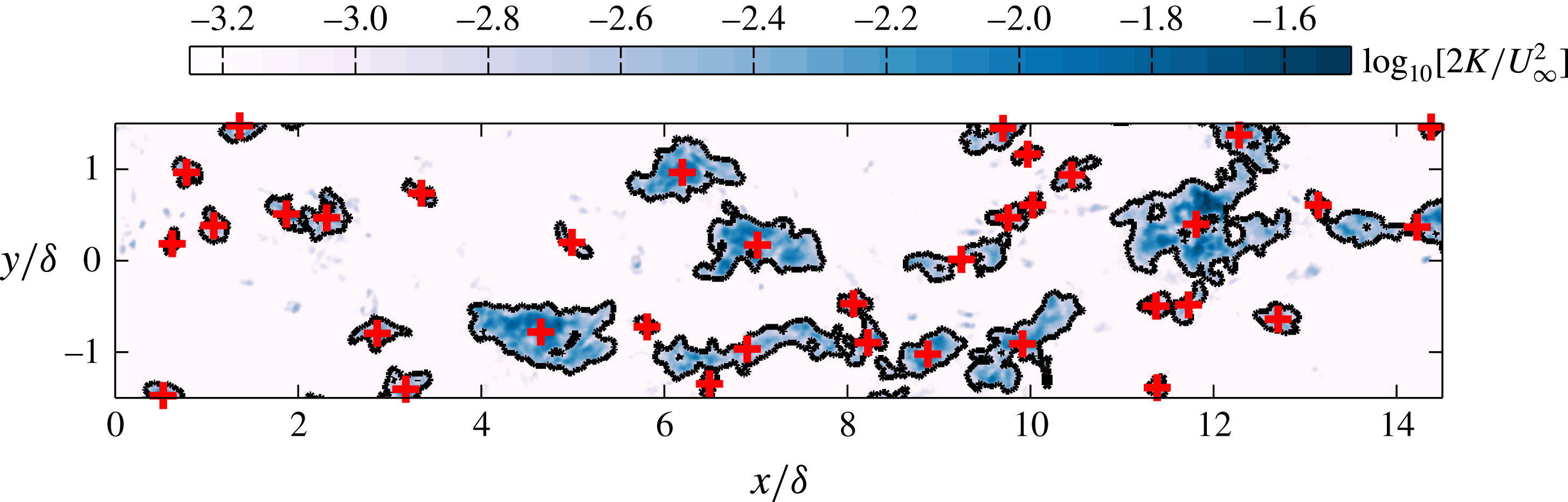
Figure 12. Instantaneous colour contours of the kinetic energy deficit,
 $K$
, for the same velocity field as shown in figure 1(a). Results are presented on an
$K$
, for the same velocity field as shown in figure 1(a). Results are presented on an
 $xy$
plane at
$xy$
plane at
 $z\approx \unicode[STIX]{x1D6FF}$
and colour levels are presented on a logarithmic scale. The solid black line indicates the location of the TNTI computed as an iso-kinetic energy surface using a threshold of
$z\approx \unicode[STIX]{x1D6FF}$
and colour levels are presented on a logarithmic scale. The solid black line indicates the location of the TNTI computed as an iso-kinetic energy surface using a threshold of
 $K_{0}=10^{-3}((1/2)U_{\infty }^{2})$
and the
$K_{0}=10^{-3}((1/2)U_{\infty }^{2})$
and the
 $+$
symbols correspond to the centroid of each detected region.
$+$
symbols correspond to the centroid of each detected region.
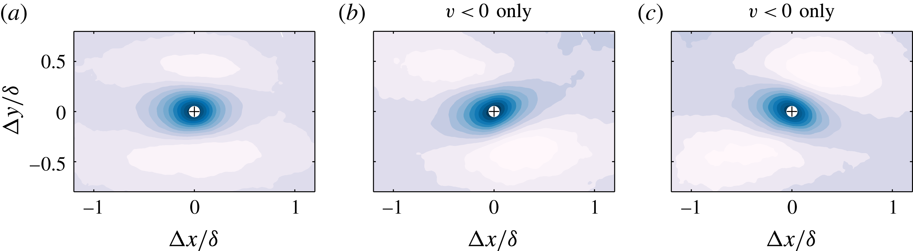
Figure 13. Conditionally averaged maps of the kinetic energy deficit,
 $\langle K\rangle$
, in the near vicinity of turbulent bulges on an
$\langle K\rangle$
, in the near vicinity of turbulent bulges on an
 $xy$
plane at
$xy$
plane at
 $z\approx \unicode[STIX]{x1D6FF}$
. In (a), all turbulent bulges are included, while in (b,c), only bulges that yield negative or positive
$z\approx \unicode[STIX]{x1D6FF}$
. In (a), all turbulent bulges are included, while in (b,c), only bulges that yield negative or positive
 $v$
respectively when averaged across the spatial extent are shown. Colour levels are presented on a logarithmic scale and are the same as in figure 12.
$v$
respectively when averaged across the spatial extent are shown. Colour levels are presented on a logarithmic scale and are the same as in figure 12.
To examine the detected turbulent bulges, statistical properties are built in the near vicinity of these features with a frame of reference attached to their centroids (see figure 12). Figure 13(a) represents the conditionally averaged kinetic energy deficit in the near vicinity of the detected turbulent bulges at
 $z\approx \unicode[STIX]{x1D6FF}$
, where, as expected, we see that these turbulent bulges span approximately
$z\approx \unicode[STIX]{x1D6FF}$
, where, as expected, we see that these turbulent bulges span approximately
 $1$
–
$1$
–
 $2\unicode[STIX]{x1D6FF}$
on average and appear to be aligned to the mean flow direction. In figure 13(b,c), however, we include only regions where the average spanwise velocity fluctuation,
$2\unicode[STIX]{x1D6FF}$
on average and appear to be aligned to the mean flow direction. In figure 13(b,c), however, we include only regions where the average spanwise velocity fluctuation,
 $v$
, within each turbulent bulge is either negative or positive. These results indicate that the orientation of the turbulent bulges is indeed affected by the obliqueness of the
$v$
, within each turbulent bulge is either negative or positive. These results indicate that the orientation of the turbulent bulges is indeed affected by the obliqueness of the
 $v$
coherence, and the streamwise-aligned representation shown in figure 13(a) is a superposition between equally frequent yawed turbulent bulges. These results also concur with correlation functions presented in figure 11 for the low-streamwise-momentum events (
$v$
coherence, and the streamwise-aligned representation shown in figure 13(a) is a superposition between equally frequent yawed turbulent bulges. These results also concur with correlation functions presented in figure 11 for the low-streamwise-momentum events (
 $u<0$
), which are within the turbulent bulges.
$u<0$
), which are within the turbulent bulges.
To give a complete three-dimensional picture of how the
 $v$
coherence impacts the turbulent bulges in the intermittent region in figure 14, we plot a three-dimensional isosurface of strong positive
$v$
coherence impacts the turbulent bulges in the intermittent region in figure 14, we plot a three-dimensional isosurface of strong positive
 $v$
regions. Results are presented beyond
$v$
regions. Results are presented beyond
 $z>0.6\unicode[STIX]{x1D6FF}$
and the isosurface is extracted from a volumetric numerical database of Sillero, Jiménez & Moser (Reference Sillero, Jiménez and Moser2013) at
$z>0.6\unicode[STIX]{x1D6FF}$
and the isosurface is extracted from a volumetric numerical database of Sillero, Jiménez & Moser (Reference Sillero, Jiménez and Moser2013) at
 $Re_{\unicode[STIX]{x1D70F}}\approx 2000$
. The colour shading represents the wall-normal height and confirms that the obliqueness in the
$Re_{\unicode[STIX]{x1D70F}}\approx 2000$
. The colour shading represents the wall-normal height and confirms that the obliqueness in the
 $v$
coherence extends throughout the intermittent region of the flow and influences the orientation of the turbulent bulges at the edge of the layer (darker shaded regions). This, in turn, produces a signature of these oblique features on the three-dimensional geometry of the TNTI (red ellipses in figure 14).
$v$
coherence extends throughout the intermittent region of the flow and influences the orientation of the turbulent bulges at the edge of the layer (darker shaded regions). This, in turn, produces a signature of these oblique features on the three-dimensional geometry of the TNTI (red ellipses in figure 14).

Figure 14. (a) The three-dimensional isosurface of strong positive
 $v$
regions (
$v$
regions (
 $v>\unicode[STIX]{x1D70E}_{v}$
), which exhibits clear preferential orientation of the
$v>\unicode[STIX]{x1D70E}_{v}$
), which exhibits clear preferential orientation of the
 $v$
coherence across the entire intermittent region. Results are presented from a direct numerical simulation database of Sillero et al. (Reference Sillero, Jiménez and Moser2013) at
$v$
coherence across the entire intermittent region. Results are presented from a direct numerical simulation database of Sillero et al. (Reference Sillero, Jiménez and Moser2013) at
 $Re_{\unicode[STIX]{x1D70F}}\approx 2000$
above
$Re_{\unicode[STIX]{x1D70F}}\approx 2000$
above
 $z>0.6\unicode[STIX]{x1D6FF}$
, and the colour shading corresponds to the wall-normal height. (b) The corresponding three-dimensional TNTI. The red ellipses highlight the signature of the oblique features in the
$z>0.6\unicode[STIX]{x1D6FF}$
, and the colour shading corresponds to the wall-normal height. (b) The corresponding three-dimensional TNTI. The red ellipses highlight the signature of the oblique features in the
 $v$
coherence in (a) which are clearly visible in the geometry of the TNTI in (b).
$v$
coherence in (a) which are clearly visible in the geometry of the TNTI in (b).
6 Observations from the attached eddy model
In § 3.1, we showed that the conditional velocity vector fields based on strong
 $v$
events in the wake region resemble a pair of inclined symmetrical vortices, at least in an average sense when both the strong positive and negative
$v$
events in the wake region resemble a pair of inclined symmetrical vortices, at least in an average sense when both the strong positive and negative
 $v$
contributions are considered. Based on these observations and inspired by the attached eddy hypothesis (Townsend Reference Townsend1976) and attached eddy model (Marusic & Perry Reference Marusic and Perry1995; Perry & Marusic Reference Perry and Marusic1995), here we test whether
$v$
contributions are considered. Based on these observations and inspired by the attached eddy hypothesis (Townsend Reference Townsend1976) and attached eddy model (Marusic & Perry Reference Marusic and Perry1995; Perry & Marusic Reference Perry and Marusic1995), here we test whether
 $\unicode[STIX]{x1D6EC}$
-shaped eddies, which essentially are pairs of inclined vortices, distributed randomly in the plane of the wall can produce similar behaviour for the coherence of
$\unicode[STIX]{x1D6EC}$
-shaped eddies, which essentially are pairs of inclined vortices, distributed randomly in the plane of the wall can produce similar behaviour for the coherence of
 $v$
to that observed in § 3.
$v$
to that observed in § 3.
To construct the synthetic velocity fields from the attached eddy model (hereafter referred to as the AEM velocity fields), a packet of
 $\unicode[STIX]{x1D6EC}$
-shaped eddies is used as a representative eddy. It must be stressed that the shape of the representative eddy has not been chosen in order to produce a particular statistical behaviour or to satisfy a particular outcome. Instead, the representative eddy shapes and sizes prescribed in this study follow prior works using the model (see Marusic Reference Marusic2001; Baidya et al.
Reference Baidya, Philip, Monty, Hutchins and Marusic2014; Woodcock & Marusic Reference Woodcock and Marusic2015 and de Silva et al.
Reference de Silva, Hutchins and Marusic2016a
). The vortex rods that constitute each
$\unicode[STIX]{x1D6EC}$
-shaped eddies is used as a representative eddy. It must be stressed that the shape of the representative eddy has not been chosen in order to produce a particular statistical behaviour or to satisfy a particular outcome. Instead, the representative eddy shapes and sizes prescribed in this study follow prior works using the model (see Marusic Reference Marusic2001; Baidya et al.
Reference Baidya, Philip, Monty, Hutchins and Marusic2014; Woodcock & Marusic Reference Woodcock and Marusic2015 and de Silva et al.
Reference de Silva, Hutchins and Marusic2016a
). The vortex rods that constitute each
 $\unicode[STIX]{x1D6EC}$
-shaped eddy are assumed to contain Gaussian distributed vorticities about their cores (Perry & Marusic Reference Perry and Marusic1995), and to obtain the velocity field, Biot–Savart calculations are performed over all vortex rods present in a single representative eddy. Thereafter, to include a hierarchical length-scale distribution of eddies, the resultant velocity field from one representative eddy is scaled physically with the wall as the origin and then randomly distributed in the plane of the wall. This process is then repeated for each hierarchical length scale.
$\unicode[STIX]{x1D6EC}$
-shaped eddy are assumed to contain Gaussian distributed vorticities about their cores (Perry & Marusic Reference Perry and Marusic1995), and to obtain the velocity field, Biot–Savart calculations are performed over all vortex rods present in a single representative eddy. Thereafter, to include a hierarchical length-scale distribution of eddies, the resultant velocity field from one representative eddy is scaled physically with the wall as the origin and then randomly distributed in the plane of the wall. This process is then repeated for each hierarchical length scale.
The placement of each packet eddy in the plane of the wall is random, with a mandated minimum distance between any two eddies (see de Silva et al.
Reference de Silva, Woodcock, Hutchins and Marusic2016b
), whereas the height of each packet eddy follows a p.d.f. that adheres to the geometric progression stated in Perry, Henbest & Chong (Reference Perry, Henbest and Chong1986). These distributions ensure that a log law is returned for the mean flow and
 $\overline{u^{2}}$
statistics. Further, the spatial population density of eddies is chosen such that we obtain the log-law constants to match the experimental results (with
$\overline{u^{2}}$
statistics. Further, the spatial population density of eddies is chosen such that we obtain the log-law constants to match the experimental results (with
 $\unicode[STIX]{x1D705}\approx 0.39$
and
$\unicode[STIX]{x1D705}\approx 0.39$
and
 $A\approx 4.3$
), and the velocity fluctuations are scaled such that the peak in the viscous scaled Reynolds shear stress is unity in the logarithmic region, which has been empirically observed at sufficiently high Reynolds numbers (Buschmann, Indinger & Gad-el-Hak Reference Buschmann, Indinger and Gad-el-Hak2009). It is worth highlighting that we have not attempted to match all of the mean flow and Reynolds stresses from the synthetic datasets (see Marusic & Perry Reference Marusic and Perry1995 and Perry & Marusic Reference Perry and Marusic1995) to the experiments. Instead, our focus here is on examining the
$A\approx 4.3$
), and the velocity fluctuations are scaled such that the peak in the viscous scaled Reynolds shear stress is unity in the logarithmic region, which has been empirically observed at sufficiently high Reynolds numbers (Buschmann, Indinger & Gad-el-Hak Reference Buschmann, Indinger and Gad-el-Hak2009). It is worth highlighting that we have not attempted to match all of the mean flow and Reynolds stresses from the synthetic datasets (see Marusic & Perry Reference Marusic and Perry1995 and Perry & Marusic Reference Perry and Marusic1995) to the experiments. Instead, our focus here is on examining the
 $v$
coherence from the model, where the range of eddy sizes can be prescribed, and how it compares with our experimental findings. More extensive details on the computational process to generate the synthetic databases and scaling of the velocity fields can be found in de Silva et al. (Reference de Silva, Hutchins and Marusic2016a
).
$v$
coherence from the model, where the range of eddy sizes can be prescribed, and how it compares with our experimental findings. More extensive details on the computational process to generate the synthetic databases and scaling of the velocity fields can be found in de Silva et al. (Reference de Silva, Hutchins and Marusic2016a
).

Figure 15. Colour contours of spanwise velocity fluctuations,
 $v$
, from an AEM synthetic velocity field at
$v$
, from an AEM synthetic velocity field at
 $Re_{\unicode[STIX]{x1D70F}}\approx 3200$
. Results are presented on streamwise/spanwise planes acquired (a) at
$Re_{\unicode[STIX]{x1D70F}}\approx 3200$
. Results are presented on streamwise/spanwise planes acquired (a) at
 $z\approx \unicode[STIX]{x1D6FF}$
and (b) in the logarithmic region (
$z\approx \unicode[STIX]{x1D6FF}$
and (b) in the logarithmic region (
 $z\approx 0.1\unicode[STIX]{x1D6FF}$
). The top, middle and bottom rows for each wall-normal location show the same flow field unconditioned and decomposed by the sign of
$z\approx 0.1\unicode[STIX]{x1D6FF}$
). The top, middle and bottom rows for each wall-normal location show the same flow field unconditioned and decomposed by the sign of
 $v$
, i.e. top
$v$
, i.e. top
 $v$
, middle
$v$
, middle
 $v<0$
and bottom
$v<0$
and bottom
 $v>0$
. The black dashed lines in (a) correspond to an inclination angle of
$v>0$
. The black dashed lines in (a) correspond to an inclination angle of
 $\pm 45^{\circ }$
with respect to the flow direction,
$\pm 45^{\circ }$
with respect to the flow direction,
 $x$
, and are only included for illustrative purposes.
$x$
, and are only included for illustrative purposes.
For the present study, the AEM velocity fields are generated at a fixed Reynolds number of
 $Re_{\unicode[STIX]{x1D70F}}=3200$
, which is comparable to that analysed experimentally. Further, the spatial resolution (or grid spacing) and spatial domain size of the velocity fields are matched to the experimental databases. An in-depth analysis of these parameters can be found in de Silva et al. (Reference de Silva, Hutchins and Marusic2016a
). To ensure a sufficient degree of convergence, each dataset consists of 500 independent volumes from which wall-parallel slices are extracted at the same wall-normal locations as available from the experiments.
$Re_{\unicode[STIX]{x1D70F}}=3200$
, which is comparable to that analysed experimentally. Further, the spatial resolution (or grid spacing) and spatial domain size of the velocity fields are matched to the experimental databases. An in-depth analysis of these parameters can be found in de Silva et al. (Reference de Silva, Hutchins and Marusic2016a
). To ensure a sufficient degree of convergence, each dataset consists of 500 independent volumes from which wall-parallel slices are extracted at the same wall-normal locations as available from the experiments.
6.1 Spanwise velocity structures in the AEM
A wall-parallel slice of an AEM velocity field is shown in figure 15. The colour contours correspond to spanwise velocity fluctuations,
 $v$
, and the Reynolds number and wall height are chosen to match the experimental velocity field shown previously in figure 1. Qualitatively, the AEM and experimental velocity fields appear to be comparable; however, one notable difference is the lack of small-scale activity in the model, as only the largest
$v$
, and the Reynolds number and wall height are chosen to match the experimental velocity field shown previously in figure 1. Qualitatively, the AEM and experimental velocity fields appear to be comparable; however, one notable difference is the lack of small-scale activity in the model, as only the largest
 $\unicode[STIX]{x1D6FF}$
-scaled eddies are visible at the top edge of the layer in figure 15(a). However, despite these differences, the AEM velocity fields appear to reproduce the
$\unicode[STIX]{x1D6FF}$
-scaled eddies are visible at the top edge of the layer in figure 15(a). However, despite these differences, the AEM velocity fields appear to reproduce the
 $\unicode[STIX]{x1D6FF}$
-scaled oblique features in the spanwise coherence similarly to our experimental findings. This behaviour is likely to be associated with the
$\unicode[STIX]{x1D6FF}$
-scaled oblique features in the spanwise coherence similarly to our experimental findings. This behaviour is likely to be associated with the
 $v$
signature at the top edge of a slanted
$v$
signature at the top edge of a slanted
 $\unicode[STIX]{x1D6EC}$
-shaped eddy, which we employ as our representative eddy shape (see figure 16
b,d). Moreover, although the
$\unicode[STIX]{x1D6EC}$
-shaped eddy, which we employ as our representative eddy shape (see figure 16
b,d). Moreover, although the
 $\unicode[STIX]{x1D6FF}$
-scaled eddies in the AEM velocity fields are randomly located relative to one another, visually they appear to form clusters aligned at
$\unicode[STIX]{x1D6FF}$
-scaled eddies in the AEM velocity fields are randomly located relative to one another, visually they appear to form clusters aligned at
 $\pm 45^{\circ }$
(denoted by black dashed lines in figure 15) for much longer extents. These observations provide further support to our findings in § 3.3, where beyond
$\pm 45^{\circ }$
(denoted by black dashed lines in figure 15) for much longer extents. These observations provide further support to our findings in § 3.3, where beyond
 ${\sim}1{-}2\unicode[STIX]{x1D6FF}$
the oblique patterns of the
${\sim}1{-}2\unicode[STIX]{x1D6FF}$
the oblique patterns of the
 $v$
coherence are not statistically correlated with one another, even though they might appear to be when visually inspecting velocity fields.
$v$
coherence are not statistically correlated with one another, even though they might appear to be when visually inspecting velocity fields.
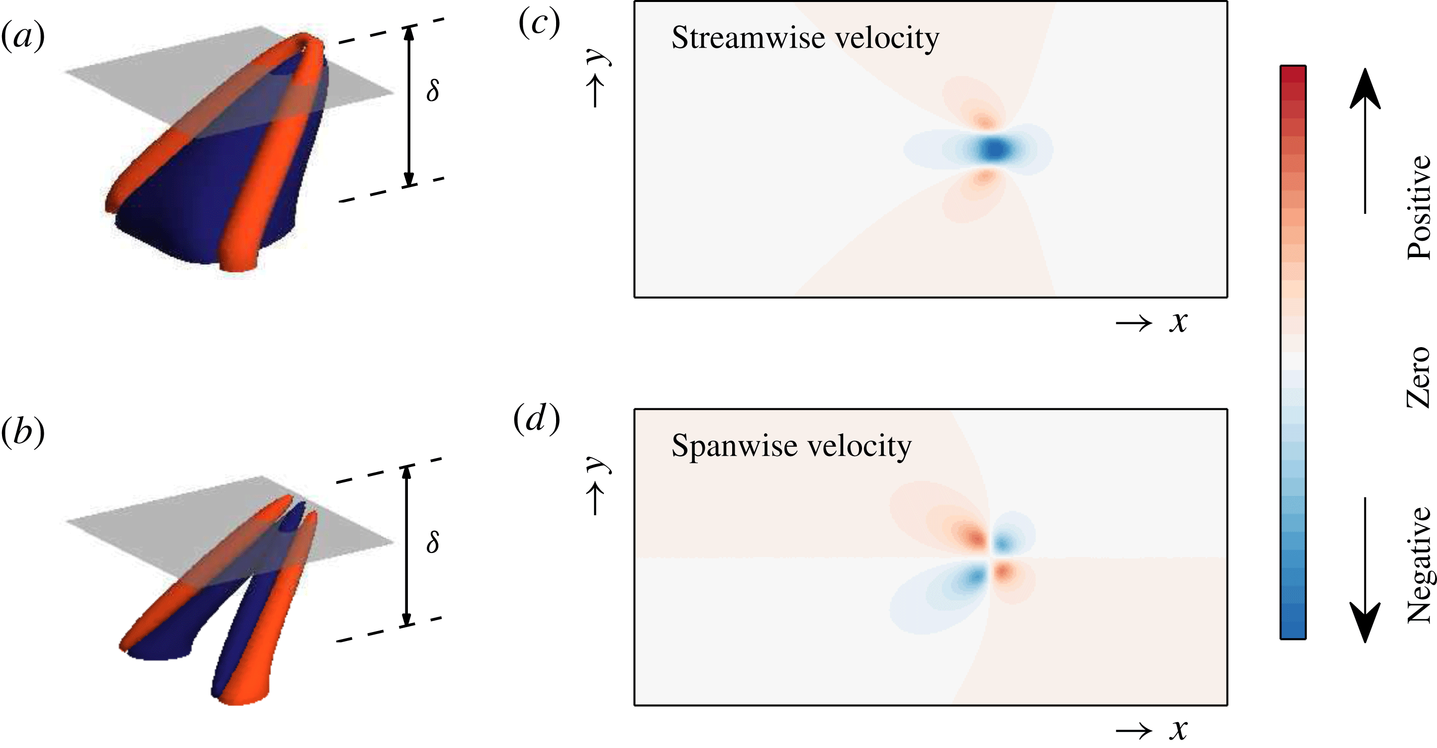
Figure 16. (a) Schematic of a typical representative
 $\unicode[STIX]{x1D6EC}$
eddy, where the blue region isolates the low-streamwise-momentum region that forms beneath the
$\unicode[STIX]{x1D6EC}$
eddy, where the blue region isolates the low-streamwise-momentum region that forms beneath the
 $\unicode[STIX]{x1D6EC}$
eddy and the red region corresponds to a higher-streamwise-momentum region. (b) The corresponding spanwise velocity, where the blue and red regions correspond to strong positive and negative spanwise velocity fluctuations respectively. (c,d) Colour contours of the streamwise and spanwise velocity contributions respectively, from the
$\unicode[STIX]{x1D6EC}$
eddy and the red region corresponds to a higher-streamwise-momentum region. (b) The corresponding spanwise velocity, where the blue and red regions correspond to strong positive and negative spanwise velocity fluctuations respectively. (c,d) Colour contours of the streamwise and spanwise velocity contributions respectively, from the
 $\unicode[STIX]{x1D6EC}$
eddies shown in (a,b). The contour levels are equal for both velocity components and are computed on the wall-parallel plane highlighted in grey in (a,b) at
$\unicode[STIX]{x1D6EC}$
eddies shown in (a,b). The contour levels are equal for both velocity components and are computed on the wall-parallel plane highlighted in grey in (a,b) at
 $z\approx 0.9\unicode[STIX]{x1D6FF}$
.
$z\approx 0.9\unicode[STIX]{x1D6FF}$
.
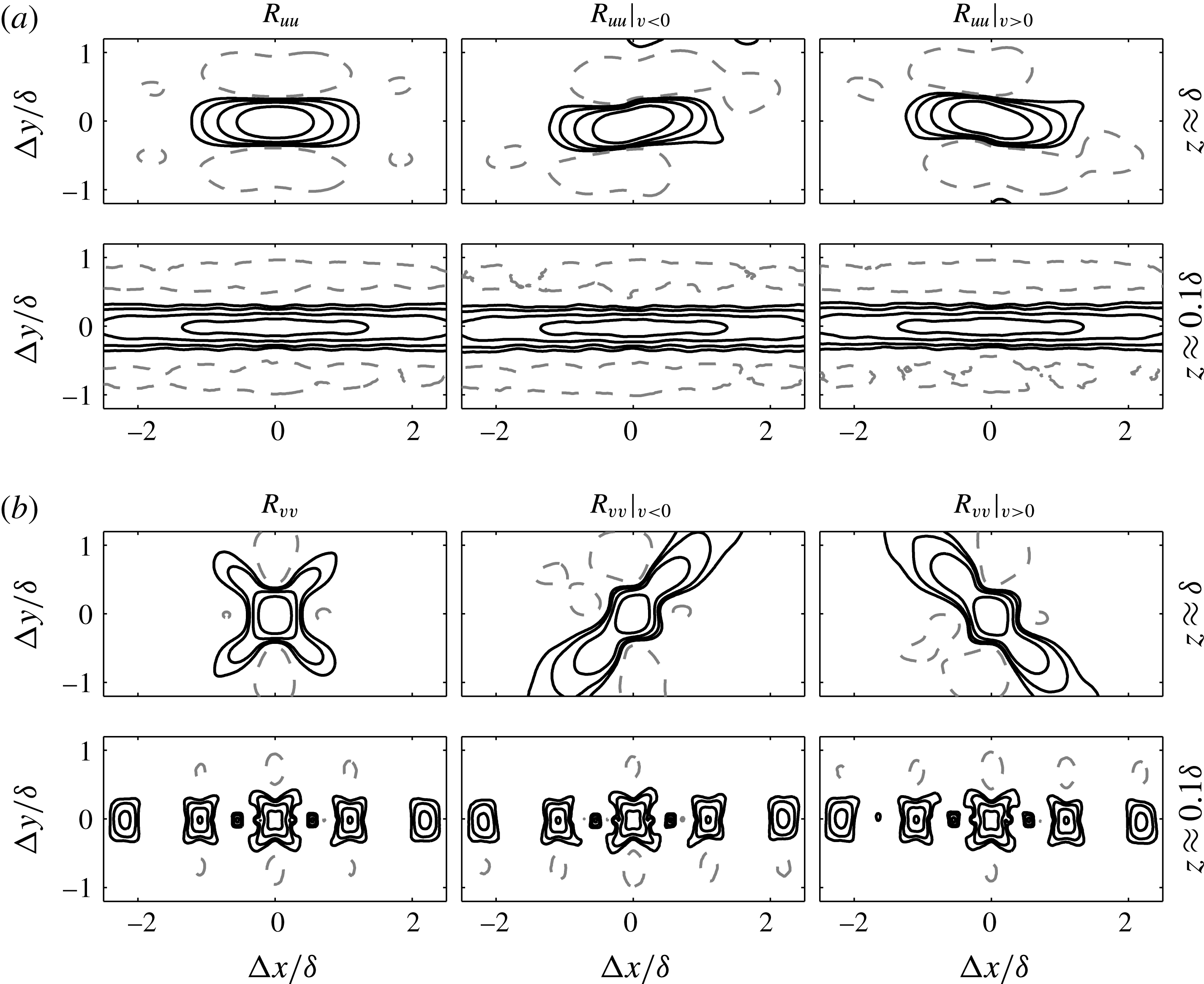
Figure 17. Wall-parallel slices of the correlation function for the (a) streamwise and (b) spanwise velocity fluctuations from the AEM velocity fields. Panels present results at different wall-normal locations. The positive contours (solid lines) are 0.05, 0.1, 0.2 and 0.4 and the negative contours (dashed lines) are
 $-$
0.1. Left column present the unconditional correlation, and middle and right columns present the conditional correlation when
$-$
0.1. Left column present the unconditional correlation, and middle and right columns present the conditional correlation when
 $v<0$
and
$v<0$
and
 $v>0$
respectively.
$v>0$
respectively.
In order to quantify these observations, in a similar manner to § 3.1, normalised two-point correlation functions computed from the AEM velocity fields are presented in figure 17. The contours represent
 $R_{uu}$
and
$R_{uu}$
and
 $R_{vv}$
computed at the edge of the boundary layer (
$R_{vv}$
computed at the edge of the boundary layer (
 $z\approx \unicode[STIX]{x1D6FF}$
) and in the logarithmic region (
$z\approx \unicode[STIX]{x1D6FF}$
) and in the logarithmic region (
 $z\approx 0.1\unicode[STIX]{x1D6FF}$
), conditioned on the sign of
$z\approx 0.1\unicode[STIX]{x1D6FF}$
), conditioned on the sign of
 $v$
. Interestingly, even though we are using an average representative structure to visualise instantaneous features, the correlation functions show strong similarity to those found from the experimental databases (see figures 3 and 4) for both velocity components. More specifically, at the edge of the boundary layer (
$v$
. Interestingly, even though we are using an average representative structure to visualise instantaneous features, the correlation functions show strong similarity to those found from the experimental databases (see figures 3 and 4) for both velocity components. More specifically, at the edge of the boundary layer (
 $z\approx \unicode[STIX]{x1D6FF}$
), the
$z\approx \unicode[STIX]{x1D6FF}$
), the
 $v$
coherence appears to be preferentially aligned at
$v$
coherence appears to be preferentially aligned at
 $\pm 45^{\circ }$
depending on the sign of
$\pm 45^{\circ }$
depending on the sign of
 $v$
, while closer to the wall, this behaviour is less pronounced. Similarly, for
$v$
, while closer to the wall, this behaviour is less pronounced. Similarly, for
 $R_{uu}$
, in addition to the streamwise elongated coherence associated with a packet-like structure (Marusic Reference Marusic2001) in the logarithmic region, we observe a slight degree of preferential orientation based on the sign of
$R_{uu}$
, in addition to the streamwise elongated coherence associated with a packet-like structure (Marusic Reference Marusic2001) in the logarithmic region, we observe a slight degree of preferential orientation based on the sign of
 $v$
at the edge of the boundary layer. This behaviour is associated with the
$v$
at the edge of the boundary layer. This behaviour is associated with the
 $u$
signature at the top edge of a single
$u$
signature at the top edge of a single
 $\unicode[STIX]{x1D6EC}$
-shaped eddy (see figure 16
c) once conditioned on the sign of
$\unicode[STIX]{x1D6EC}$
-shaped eddy (see figure 16
c) once conditioned on the sign of
 $v$
. Moreover, a deconstruction of
$v$
. Moreover, a deconstruction of
 $R_{uu}$
and
$R_{uu}$
and
 $R_{vv}$
based on the signs of
$R_{vv}$
based on the signs of
 $u$
and
$u$
and
 $v$
in a similar manner to § 4 (not reproduced here) also shows comparable results to those obtained from the experiments. Collectively, from these observations, we postulate that one possible explanation that leads to oblique features in the
$v$
in a similar manner to § 4 (not reproduced here) also shows comparable results to those obtained from the experiments. Collectively, from these observations, we postulate that one possible explanation that leads to oblique features in the
 $v$
coherence with spatial extents limited to
$v$
coherence with spatial extents limited to
 $1{-}2\unicode[STIX]{x1D6FF}$
is the presence of structures similar to those prescribed in the AEM synthetic velocity fields that contain a vortex-like structure with an arch or head, which results in strong
$1{-}2\unicode[STIX]{x1D6FF}$
is the presence of structures similar to those prescribed in the AEM synthetic velocity fields that contain a vortex-like structure with an arch or head, which results in strong
 $v$
signatures that are aligned at
$v$
signatures that are aligned at
 $\pm 45^{\circ }$
in a wall-parallel plane (see figure 16
d).
$\pm 45^{\circ }$
in a wall-parallel plane (see figure 16
d).
Despite the AEM velocity fields appearing to reproduce the obliqueness in the
 $v$
coherence in this work, it must be stressed that the model does not conform to certain experimental observations. For example, the model does not accommodate any variation in the shape of the eddies contributing to the turbulence. In reality, we know from the literature (Robinson Reference Robinson1991; Schlatter et al.
Reference Schlatter, Li, Örlü, Hussain and Henningson2014, and others) that, instantaneously, large-scale coherent regions differ from the conditionally averaged features. Consequently, the distinct repeating patterns present in the instantaneous velocity fields (figure 15) are absent in experiments. Additionally, the repeating pattern visible in
$v$
coherence in this work, it must be stressed that the model does not conform to certain experimental observations. For example, the model does not accommodate any variation in the shape of the eddies contributing to the turbulence. In reality, we know from the literature (Robinson Reference Robinson1991; Schlatter et al.
Reference Schlatter, Li, Örlü, Hussain and Henningson2014, and others) that, instantaneously, large-scale coherent regions differ from the conditionally averaged features. Consequently, the distinct repeating patterns present in the instantaneous velocity fields (figure 15) are absent in experiments. Additionally, the repeating pattern visible in
 $R_{vv}$
at
$R_{vv}$
at
 $z\approx 0.1$
in the logarithmic region (see figure 17) is an artefact of maintaining a fixed spacing between the
$z\approx 0.1$
in the logarithmic region (see figure 17) is an artefact of maintaining a fixed spacing between the
 $\unicode[STIX]{x1D6EC}$
eddies that collectively form a streamwise elongated packet-like structure (see Marusic Reference Marusic2001 and de Silva et al.
Reference de Silva, Hutchins and Marusic2016a
). However, in reality, the spacing between these
$\unicode[STIX]{x1D6EC}$
eddies that collectively form a streamwise elongated packet-like structure (see Marusic Reference Marusic2001 and de Silva et al.
Reference de Silva, Hutchins and Marusic2016a
). However, in reality, the spacing between these
 $\unicode[STIX]{x1D6EC}$
eddies would vary from one packet-like structure to another, which would suppress the periodic pattern observed in
$\unicode[STIX]{x1D6EC}$
eddies would vary from one packet-like structure to another, which would suppress the periodic pattern observed in
 $R_{vv}$
.
$R_{vv}$
.
To further illustrate how the instantaneous coherent regions differ from bulk features in boundary layers, figure 18 shows colour contours of kinetic turbulent energy at
 $z\approx \unicode[STIX]{x1D6FF}$
. The results highlight that the turbulent patches from the experiments are aligned over a wide range of angles to the flow direction (red solid lines), unlike the model where
$z\approx \unicode[STIX]{x1D6FF}$
. The results highlight that the turbulent patches from the experiments are aligned over a wide range of angles to the flow direction (red solid lines), unlike the model where
 $\unicode[STIX]{x1D703}\approx 0^{\circ }$
for most turbulent patches (unless they happen to overlap) due to the nature of their placement. Similar evidence for instantaneous structures being misaligned from the main flow direction is also a common observation for
$\unicode[STIX]{x1D703}\approx 0^{\circ }$
for most turbulent patches (unless they happen to overlap) due to the nature of their placement. Similar evidence for instantaneous structures being misaligned from the main flow direction is also a common observation for
 $u$
coherence. For example, at low
$u$
coherence. For example, at low
 $Re$
, it is illustrated in the models of Jeong et al. (Reference Jeong, Hussain, Schoppa and Kim1997) and the instability mechanism of Schoppa & Hussain (Reference Schoppa and Hussain2002). Furthermore, scalar visualisation by Delo, Kelso & Smits (Reference Delo, Kelso and Smits2004) also suggests that individual turbulence bulges appear to tilt sideways. Therefore, although the obliqueness in the
$Re$
, it is illustrated in the models of Jeong et al. (Reference Jeong, Hussain, Schoppa and Kim1997) and the instability mechanism of Schoppa & Hussain (Reference Schoppa and Hussain2002). Furthermore, scalar visualisation by Delo, Kelso & Smits (Reference Delo, Kelso and Smits2004) also suggests that individual turbulence bulges appear to tilt sideways. Therefore, although the obliqueness in the
 $v$
coherence is captured by the AEM velocity fields, further refinement of the representative structures in the model would be necessary in order to better capture the instantaneous flow features. These modifications are likely to involve the inclusion of a range of representative eddies that are not necessarily forced to be streamwise-aligned or symmetric.
$v$
coherence is captured by the AEM velocity fields, further refinement of the representative structures in the model would be necessary in order to better capture the instantaneous flow features. These modifications are likely to involve the inclusion of a range of representative eddies that are not necessarily forced to be streamwise-aligned or symmetric.
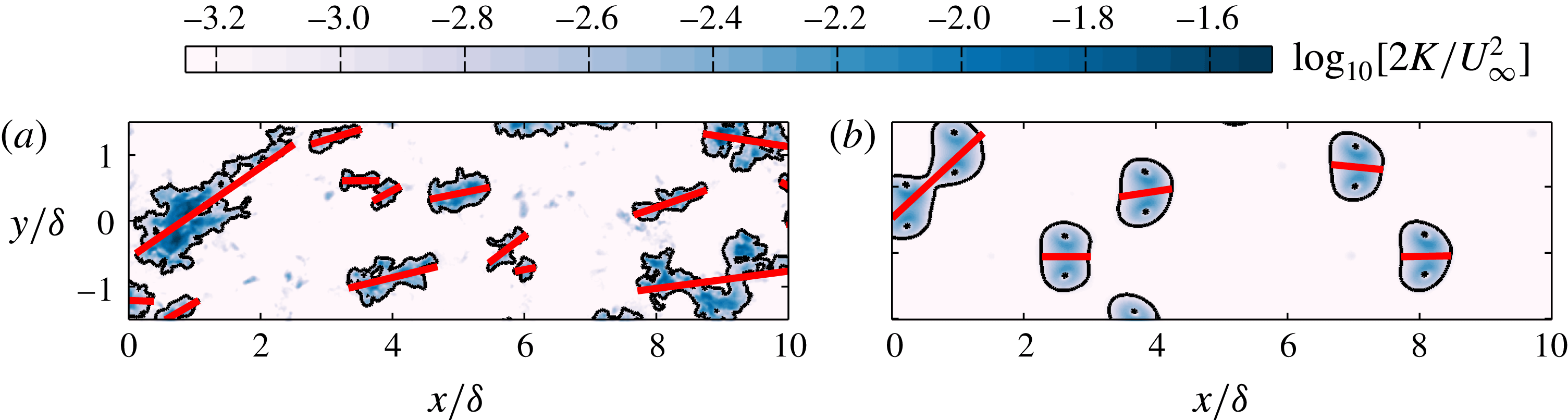
Figure 18. A comparison of instantaneous colour contours of kinetic energy,
 $K$
, between (a) an experimental and (b) an AEM velocity field on an
$K$
, between (a) an experimental and (b) an AEM velocity field on an
 $xy$
plane at
$xy$
plane at
 $z\approx \unicode[STIX]{x1D6FF}$
. The solid black line indicates the location of the TNTI. The solid red lines indicate the principal axis of each turbulent patch detected.
$z\approx \unicode[STIX]{x1D6FF}$
. The solid black line indicates the location of the TNTI. The solid red lines indicate the principal axis of each turbulent patch detected.
7 Summary and conclusions
This paper examines the large-scale oblique pattern in the spanwise velocity component in turbulent boundary layers using a set of unique large-field-of-view PIV measurements. The experiments are configured to capture a sufficiently large spatial domain of the order of several boundary layer thicknesses in both the streamwise and spanwise directions. Consistent with Sillero et al. (Reference Sillero, Jiménez and Moser2014), analysis of two-point correlation functions reveals pronounced oblique features of the spanwise coherence at the edge of the boundary layer, which are counter-oriented based on the sign of
 $v$
. These observations are shown to relate to the intermittent turbulent bulges at the edge of the layer, with the clear presence of two counter-oriented oblique features. Moreover, we find that these oblique features also extend closer to the wall and are present in the logarithmic region once the velocity fields are deconstructed based on the signs of both
$v$
. These observations are shown to relate to the intermittent turbulent bulges at the edge of the layer, with the clear presence of two counter-oriented oblique features. Moreover, we find that these oblique features also extend closer to the wall and are present in the logarithmic region once the velocity fields are deconstructed based on the signs of both
 $u$
and
$u$
and
 $v$
. Through this analysis, we show that the obliqueness is also present in the streamwise coherence, albeit more subtly. Consequently, the often-reported meandering of the
$v$
. Through this analysis, we show that the obliqueness is also present in the streamwise coherence, albeit more subtly. Consequently, the often-reported meandering of the
 $u$
coherence (Hutchins & Marusic Reference Hutchins and Marusic2007) appears to be associated with more obvious diagonal features of the spanwise coherence.
$u$
coherence (Hutchins & Marusic Reference Hutchins and Marusic2007) appears to be associated with more obvious diagonal features of the spanwise coherence.
Through a conditional correlation analysis, we also show that the obliqueness in the
 $v$
coherence is limited to within two boundary layer thicknesses, even though a purely visual inspection of velocity fields suggests that they appear to extend for very long extents. These quantitative estimates are in line with the size of the large-scale motions thought to exist in the wake region of a boundary layer (Adrian et al.
Reference Adrian, Meinhart and Tomkins2000; Tomkins & Adrian Reference Tomkins and Adrian2003). Further, the conditional analysis also shows that the
$v$
coherence is limited to within two boundary layer thicknesses, even though a purely visual inspection of velocity fields suggests that they appear to extend for very long extents. These quantitative estimates are in line with the size of the large-scale motions thought to exist in the wake region of a boundary layer (Adrian et al.
Reference Adrian, Meinhart and Tomkins2000; Tomkins & Adrian Reference Tomkins and Adrian2003). Further, the conditional analysis also shows that the
 $u$
coherence of these features is comparable in size to the large regions of uniform streamwise momentum reported in boundary layers (Meinhart & Adrian Reference Meinhart and Adrian1995; de Silva et al.
Reference de Silva, Hutchins and Marusic2016a
).
$u$
coherence of these features is comparable in size to the large regions of uniform streamwise momentum reported in boundary layers (Meinhart & Adrian Reference Meinhart and Adrian1995; de Silva et al.
Reference de Silva, Hutchins and Marusic2016a
).
To complement and aid the interpretation of our findings from the experiments, synthetic velocity fields are generated by following the attached eddy model, where the boundary layer is conceived as a collection of randomly located self-similar eddies that have prescribed sizes. These synthetic datasets are shown to produce oblique features in the spanwise coherence with spatial extents similar to those observed from the experiments. More specifically, analysis of the synthetic databases reveals correlation functions and conditional statistics that resemble those from the experiments. Hence, these findings suggest that the oblique features in the spanwise coherence might result from similar structures to those used in the model, with population and length-scale distributions similar to those prescribed in the model.
Acknowledgement
The authors gratefully acknowledge the financial support of the Australian Research Council.


