


1. Introduction
Buoyancy-driven exchange flows (drainage), due to the release of a heavy mixture into a light one, are amongst the most fundamental fluid mechanics problems. These flows are found widely in nature within oceanographic, meteorological and geophysical contexts as well as in industry, e.g. continuous reactors, counter-current extraction columns, bio coating and food processing, as laid out by Birman et al. (Reference Birman, Battandier, Meiburg and Linden2007), Baird et al. (Reference Baird, Aravamudan, Rao, Chadam and Peirce1992), and Buchanan et al. (Reference Buchanan, Molenaar, de Villiers and Evans2007). Such flows may contain particles that can be classified into non-colloidal (over-micron) and colloidal regimes (sub-micron). Recently, the non-colloidal exchange flows were investigated experimentally by Mirzaeian & Alba (Reference Mirzaeian and Alba2018b) as well as theoretically (thin-film lubrication model) for monodensity and bidensity suspensions by Mirzaeian & Alba (Reference Mirzaeian and Alba2018a) and Mirzaeian, Testik & Alba (Reference Mirzaeian, Testik and Alba2020), respectively, exhibiting completely distinct flow patterns and interface shapes compared to the particle-free (pure fluid) case of Seon et al. (Reference Seon, Hulin, Salin, Perrin and Hinch2005). Depending on the governing flow parameters, rich and/or depleted areas of particle concentration have been identified. The advancement interpenetration speed of the heavy and light phases are further quantified in these studies. Note that non-colloidal particle-laden flows within confined (duct) geometries studied by Mirzaeian & Alba (Reference Mirzaeian and Alba2018a) and Mirzaeian et al. (Reference Mirzaeian, Testik and Alba2020), furthermore, exhibit distinct behaviour compared to their free-surface flow counterparts examined by Zhou et al. (Reference Zhou, Dupuy, Bertozzi and Hosoi2005) and Cook, Bertozzi & Hosoi (Reference Cook, Bertozzi and Hosoi2008). For instance, gravity-driven free-surface particulate film flow experiments and theory of Zhou et al. (Reference Zhou, Dupuy, Bertozzi and Hosoi2005) and Cook et al. (Reference Cook, Bertozzi and Hosoi2008) disclose a somewhat one-step increase in volume fraction of particles near the front due to heavy particle settling. However, in confined duct geometry, an elaborate two-step increase pattern in particle concentration is observed along the stretched heavy–light interface, which is discussed by Mirzaeian & Alba (Reference Mirzaeian and Alba2018a).
The mechanism of particle transport in a non-colloidal (non-Brownian) regime – e.g. probed by Murisic et al. (Reference Murisic, Ho, Hu, Latterman, Koch, Lin, Mata and Bertozzi2011), Mirzaeian & Alba (Reference Mirzaeian and Alba2018a), and Mirzaeian et al. (Reference Mirzaeian, Testik and Alba2020) – is through settling and/or shear-induced migration. However, a recent analytical study of Espín & Kumar (Reference Espín and Kumar2014), conducted for colloidal (nanoparticle) thin-film flows over an inclined plane with coating application, reveals novel diffusive transport via hydrodynamic interactions as well as osmotic pressure. Fascinating interface patterns stemming from the streamwise particle diffusion and viscosity field modification are reported. For sufficiently high Péclet numbers, defined as the ratio of advective to diffusive transport rates, even minute inhomogeneities in initial concentration of particles may result in viscosity gradients that can cause continuous evolvement and thinning of the film front instead of travelling without shape change as happens in the particle-free case. Particle diffusion at high volume fractions can further result in the formation of long-lasting secondary flow fronts in thin-film and coating currents, as discussed by Espín & Kumar (Reference Espín and Kumar2014). Channelled flow patterns are, furthermore, reported in experiments of Buchanan et al. (Reference Buchanan, Molenaar, de Villiers and Evans2007) on draining flows of colloidal thin films. The spontaneous formation of these channels is associated with the presence of low-particle-concentration zones flowing faster than the surrounding regions. Colloidal film flows can explain other complex phenomena such as contact-line pinning, skin formation and coffee-ring effects as explained by Craster, Matar & Sefiane (Reference Craster, Matar and Sefiane2009) and Maki & Kumar (Reference Maki and Kumar2011).
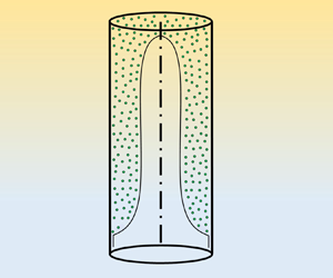
As a novel approach, we adopt the methodology of Espín & Kumar (Reference Espín and Kumar2014) on free-surface colloidal film flows over inclined plates, and extend it to the practical confined duct geometry of Mirzaeian & Alba (Reference Mirzaeian and Alba2018a) and Mirzaeian et al. (Reference Mirzaeian, Testik and Alba2020) (two-dimensional (2-D) channel simulations along with axisymmetric pipe formulation are given in Appendix B). Note that the particles are assumed to be hard spheres. Another novelty of this work is explained here. In the study of Espín & Kumar (Reference Espín and Kumar2014), due to negligible viscosity of air, the shear stress at the suspension film interface is ignored. In the current work, however, a framework to handle non-zero shear stress at the interface is developed. In other words, a viscous drainage fluid flow is considered that can relate to a wider range of applications and processes. Figure 1 shows the schematic release of such a viscous drainage problem. In this paper, we aim to provide a robust predictive framework capturing the dynamics of heavy–light interpenetrating flows in the presence of fine colloidal nanoparticles. The derived model encompasses a range of important dimensionless numbers that make systematic study of fluid flow possible. These governing parameters are listed here as the Péclet number, precursor film thickness, Reynolds number, mixtures’ viscosity ratio, initial volume fraction of particles, particles concentration within the precursor film, and capillary number. The thin-film model formulation is provided in § 2. Numerical methodology to solve the outcome model is explained in § 3, followed by benchmarking in § 4, and computational results laid out in § 5. Concluding remarks are provided in § 6.

Figure 1. Schematic of colloidal exchange flow (viscous drainage due to buoyancy) in (a) a vertical 2-D channel, and (b) an axisymmetric pipe (see Appendix B). The shape of the interface between the heavy and light mixtures is illustrative only.
2. Thin-film flow formulation
The problem shown schematically in figure 1 involves 11 dimensional parameters that we denote using the  $\hat {~}$ symbol (dimensionless parameters are identified consistently without
  $\hat {~}$ symbols throughout the paper). The gravitational acceleration is specified by
  $\hat {g}$. The vertical duct's width and length are
  $2\hat {D}$ and
  $\hat {L}$, respectively (note that
  $\hat {L} \gg 2 \hat {D}$ for the thin-film limit considered). The solid particles are assumed to be hard (incompressible) and spherical with typical diameter less than a micron (colloid). The diffusion coefficient of particles within the suspension phase is
  $\hat {D}_0$, obtainable from the Stokes–Einstein equation expressed by Russel, Saville & Schowalter (Reference Russel, Saville and Schowalter1989). The heavy suspension has density
  $\hat {\rho }_{H}$. The carrying fluid of heavy suspension is Newtonian and has viscosity
  $\hat {\mu }_{f,H}$. Similar to the modelling approach of Espín & Kumar (Reference Espín and Kumar2014) and Pham & Kumar (Reference Pham and Kumar2017), particle sedimentation is assumed to be negligible, which may be interpreted as the density of particles being close to that of the suspension-carrying fluid. The density and viscosity of the Newtonian light fluid, which is immiscible with the heavy one, are expressed as
  $\hat {\rho }_{L}$ and
  $\hat {\mu }_{L}$, respectively. Similar to the solid phase, the fluid phases are taken to be incompressible as well. The total initial volume of particles is
  $\hat {V}_p$. At time
  $\hat {t}=0$ s, the heavy-particle-laden mixture takes the top half of the duct (
 $\hat {x} \leqslant 0$), whereas the light pure fluid one occupies the bottom half (
 $\hat {x} > 0$). The jamming volume of particles is further assigned by
  $\hat {V}_j$. The interfacial tension between the heavy and light mixtures is denoted by
  $\hat {\sigma }$. The suspension layer perfectly wets the duct's surface through a narrow precursor film, whereas the light fluid is assumed to have non-wetting properties. Through a standard Buckingham-
 ${\rm \pi}$ theorem and dimensional analysis, one may arrive at eight dimensionless parameters controlling the flow in question: duct aspect ratio
  $\delta =\hat {D}/\hat {L}$, Péclet number
  $Pe = \hat {V}_t \hat {L}/\hat {D}_0$, light-to-heavy-fluid density ratio
  $\psi =\hat {\rho }_L/\hat {\rho }_{H}$, light-to-carrying-fluid viscosity ratio
  $\kappa =\hat {\mu }_L/\hat {\mu }_{f,H}$, initial volume fraction of particles
  $\varPhi _i=\hat V_p/\hat {V}_H$, jamming volume fraction
  $\varPhi _j=\hat {V}_j/\hat {V}_H$, Reynolds number
  $Re=\hat \rho _{H} {{\hat {V}}_t}(2\hat {D})/{\hat {\mu }}_H( {{\varPhi _i}} )$, and capillary number
  $Ca^{\star }=\hat {\mu }_H (\varPhi _i)\,\hat {V}_t/\hat {\sigma }$. Note that the scaling methodology of our lubrication model (to be explained in § 2) stems from small duct aspect ratio
  $\delta$, not necessarily vanishingly low
  $Re$. However, the chosen range of
  $Re$ in the simulations of § 5 is within order 1, which well suggests a laminar flow assumption consistent with the lubrication model.
Assuming that the duct has unit depth, the total volume of the heavy solution is  $\hat {V}_H=\hat {D} \hat {L}$. Moreover, the jamming volume fraction is
  $\varPhi _j \approx 0.64$ as adopted by Espín & Kumar (Reference Espín and Kumar2014). The Krieger–Dougherty expression
  ${\hat {\mu } }_H( {{\varPhi _i}} )={\hat {\mu } }_{f,H}{{( {1 - {\varPhi _i}/{\varPhi _j}} )}^{ - 2}}$ determines the heavy suspension viscosity that is implemented in the work of Mirzaeian et al. (Reference Mirzaeian, Testik and Alba2020) (see also figure 2). The characteristic velocity in the Péclet number, Reynolds number and capillary number expressions is defined as
  ${\hat V}_t=\sqrt {{{\hat {g}\hat {D} ( \hat {\rho }_H-\hat {\rho }_L )}}/{{( \hat {\rho }_H+\hat {\rho }_L )}}}$. As mentioned in the works of Mirzaeian & Alba (Reference Mirzaeian and Alba2018a,Reference Mirzaeian and Albab) and Mirzaeian et al. (Reference Mirzaeian, Testik and Alba2020), during the early flow development stage, the buoyant stress
  $(\hat {\rho }_H-\hat {\rho }_L)\hat {g}\hat {D}$ is balanced by inertial stress
  $(\hat {\rho }_H+\hat {\rho }_L)\hat {V}^{2}$, which results in obtaining the
  ${\hat V}_t$ characteristic speed. Note that the non-colloidal model of Mirzaeian & Alba (Reference Mirzaeian and Alba2018a) and Mirzaeian et al. (Reference Mirzaeian, Testik and Alba2020) has been developed in the Stokes limit of
  $r_p^{2}\,Re \ll At \ll \delta \ll 1$ with small Atwood number
  $At=(1-\psi )/(1+\psi )$, invoking the Boussinesq approximation and authorizing negligible shear-induced migration effects. The parameter
  $r_p$ is the ratio of particle radius to half the duct width. Moreover, in the studies of Mirzaeian & Alba (Reference Mirzaeian and Alba2018a) and Mirzaeian et al. (Reference Mirzaeian, Testik and Alba2020), the condition
  $r_p^{2} Re \ll At$ justifies the use of the divergence-free condition for average velocity within the suspension layer; refer to the scaling argument of Birman et al. (Reference Birman, Battandier, Meiburg and Linden2007) as well as the multiphase continuity equations of Birman et al. (Reference Birman, Martin, Meiburg and Linden2005) and Bonometti, Balachandar & Magnaudet (Reference Bonometti, Balachandar and Magnaudet2008). However, the colloidal model to be developed later in this paper is fundamentally different than the models of Mirzaeian & Alba (Reference Mirzaeian and Alba2018a) and Mirzaeian et al. (Reference Mirzaeian, Testik and Alba2020), since the particle density is chosen close to that of the carrying fluid. As a result, the model (not limited to the Boussinesq case) follows automatically the divergence-free velocity field.


Due to the symmetry, only half of the duct domain ( $0 \leqslant y \leqslant 1$) is considered (figure 1a). Following the recent thin-film approach of Hasnain & Alba (Reference Hasnain and Alba2017) for confined two-layer flows, the governing streamwise and depthwise momentum equations in the heavy-particle-laden layer read
 $$\begin{gather} 0 ={-} {p_x} + \frac{Re}{{1 - \psi }} + (\mu_H(\varPhi)\,u_y )_y, \end{gather}$$
 $$\begin{gather}0 ={-} {p_y}, \end{gather}$$
where the streamwise and depthwise distances have been scaled by  $\hat {D}/\delta$ and
  $\hat {D}$, respectively. The pressure has further been scaled by
  $\hat {\mu }_H (\varPhi _i)\, \hat {V}_t/(\delta \hat {D})$. The dimensionless viscosity of the heavy layer in the continuum form and as a function of the particles volume fraction
  $\varPhi$, is expressed below as laid out by Espín & Kumar (Reference Espín and Kumar2014) and Mirzaeian & Alba (Reference Mirzaeian and Alba2018a):
 \begin{equation} {\mu _H}( \varPhi ) =\frac{\left( {1 - \varPhi/\varPhi_j} \right)^{ - 2}}{\left( {1 - \varPhi_i/\varPhi_j} \right)^{ - 2}}.\end{equation}
The momentum equations for the Newtonian light fluid layer are provided by Hasnain & Alba (Reference Hasnain and Alba2017), Mirzaeian & Alba (Reference Mirzaeian and Alba2018a) and Mirzaeian et al. (Reference Mirzaeian, Testik and Alba2020) as
 $$\begin{gather} 0 ={-} {p_x} + \frac{\psi\,Re}{{1 - \psi }} + m{u_{yy}}, \end{gather}$$
 $$\begin{gather}0 ={-} {p_y}, \end{gather}$$
where  $m={\hat {\mu } }_L/{\hat {\mu } }_H(\varPhi _i)=\kappa {{( {1 - \varPhi _i/\varPhi _j} )}^{ 2}}$ is the ratio of the viscosity of the light fluid to that of the heavy suspension layer. Integrating (2.2) across the heavy layer depth gives
 \begin{equation} p = {p_w}( {x,t} ) + \frac{x\,Re}{{1 - \psi }},\quad 0 \leqslant y \leqslant h,\end{equation}
where we have defined a scaled wall pressure parameter,  $p_w(x,t)$, as
 \begin{equation} {p_w}( {x,t} ) = p( {x,0,t} ) - \frac{ x\,Re }{{1 - \psi }}. \end{equation}
Integrating (2.5) in the depthwise  $y$ direction gives the pressure field within the light fluid layer as
 \begin{equation} p = {p_w}( {x,t} ) + \frac{x\,Re}{{1 - \psi }}+\frac{h_{xx}}{Ca},\quad h \leqslant y \leqslant 1,\end{equation}
where  $Ca$ is a rescaled capillary number defined as
  $Ca=Ca^{\star }/ \delta ^{3}$, with
  $Ca^{\star }=\hat {\mu }_H (\varPhi _i) \hat {V}_t/\hat {\sigma }$. The capillary number rescaling allows us to retain important interfacial tension effects close to the vicinity of advancing heavy and light frontal regions in our thin-film model. Note that the capillary term impact in our model becomes relevant where there is sharp interface curvature – near the front capillary ridge elaborated by Hasnain & Alba (Reference Hasnain and Alba2017) – but disappears elsewhere as discussed by Espín & Kumar (Reference Espín and Kumar2014). The upper limit of the capillary number is dictated by the small-slope restriction of the lubrication model,
  $Ca^{1/3} \ll 1/\delta$ or
  $Ca^{\star 1/3} \ll 1$; refer to Espín & Kumar (Reference Espín and Kumar2014) for details.
The pressure expression (2.8) is now used in the streamwise momentum equations (2.1) and (2.4) to obtain
 $$\begin{gather} 0 ={-} {p_{w,x}} + (\mu_H(\varPhi)\,u_y)_y,\quad 0 \leqslant y \leqslant h, \end{gather}$$
 $$\begin{gather}0 ={-} {p_{w,x}} - Re - h_{xxx}/Ca+ m{u_{yy}},\quad h \leqslant y \leqslant 1. \end{gather}$$
Similar to the approach of Espín & Kumar (Reference Espín and Kumar2014) for free-surface colloidal films, we assume that the suspension layer wets the wall by a narrow precursor film of dimensionless thickness  $b(=\hat {b}/\hat {D})$. The precursor film, which conveniently eliminates the well-known contact-line shear stress singularity discussed by Hasnain & Alba (Reference Hasnain and Alba2017), has indeed been observed in numerous experimental works and can range from 10 nm to
  $1\ \mathrm {\mu }{\rm m}$ in thickness, as discussed in the review work of Popescu et al. (Reference Popescu, Oshanin, Dietrich and Cazabat2012). It is assumed that the heavy film is perfectly wetting, with zero static contact angle, such that any influence of disjoining pressure, described by Espín & Kumar (Reference Espín and Kumar2014), can be neglected. Correspondingly, no-slip and stress-free conditions at the wall (
 $y=0$) and the duct centre (
 $y=1$) are applied as
 $$\begin{gather} u = 0\quad {\rm at}\ y = 0, \end{gather}$$
 $$\begin{gather}u_y= 0\quad {\rm at}\ y = 1. \end{gather}$$
The homogeneity of the velocity and shear stress at the interface ( $y=h$) reads
 \begin{equation} [u] = 0,\quad [ {{\tau _{xy}}}] = 0,\quad {\rm at}\ y = h, \end{equation}
where  $[~]$ represents the jump of a given quantity. The net zero exchange flow constraint formulated in the work of Hasnain & Alba (Reference Hasnain and Alba2017), Mirzaeian & Alba (Reference Mirzaeian and Alba2018a) and Mirzaeian et al. (Reference Mirzaeian, Testik and Alba2020) reads
 \begin{equation} \int_0^{1} u \,{{\rm d} y} = 0. \end{equation}
Following the approach of Espín & Kumar (Reference Espín and Kumar2014), the particle concentration equation in dimensionless form can be written as
 \begin{equation} {\delta ^{2}}\,Pe( {{\varPhi _{_t}} + u{\varPhi _x} + v{\varPhi _y}}) = {\delta ^{2}}{\left( {D( \varPhi )\,{\varPhi _x}} \right)_x} + {({D( \varPhi )\,{\varPhi _y}})_y}, \end{equation}
where, based on a generalized Stokes–Einstein equation,
 \begin{equation} D( \varPhi ) = \frac{{\tilde{\hat{D}}\left( \varPhi \right)}}{{{{\hat{D}}_0}}} = {\left( {1 - \varPhi } \right)^{6.55}}\,\frac{{\rm d}}{{{\rm d}\varPhi }}\left( {\frac{{1.85\varPhi }}{{{\varPhi _j} - \varPhi }}} \right) \end{equation}
is the dimensionless diffusion coefficient, with  ${{\hat {D}}_0} = {\hat {k}_B\hat {T}}/({6{\rm \pi} {\hat {\mu } _{f,H}}\hat {a}})$ being the Einstein diffusivity, and
  $\hat {a}$ the radius of colloidal particles explained by Yiantsios & Higgins (Reference Yiantsios and Higgins2006) and Espín & Kumar (Reference Espín and Kumar2014). Moreover,
  $\hat {k}_B$ and
  $\hat {T}$ are the Boltzmann constant and characteristic temperature of the system, which is assumed to be constant in our study. Merlin, Salmon & Leng (Reference Merlin, Salmon and Leng2012) propose an alternative expression for colloidal suspensions of hard spheres that can capture the diffusion phenomenon over the range
  $\varPhi \lesssim 0.5$ more accurately:
 \begin{equation} D( \varPhi ) = {\left( {1 - \varPhi } \right)^{6.55}}\,\frac{{\rm d} \left( \varPhi z(\varPhi) \right)}{{{\rm d}\varPhi }}, \end{equation}
where
 \begin{equation} z( \varPhi ) = \frac{1+a_1 \varPhi+a_2 \varPhi^{2} +a_3 \varPhi^{3}+a_4 \varPhi^{4}}{1-\varPhi/\varPhi_j}, \end{equation}
and  $a_1=4-1/\varPhi _j$,
  $a_2=10-4/\varPhi _j$,
  $a_3=18-10/\varPhi _j$, and
  $a_4=1.85/\varPhi _j^{5}-18/\varPhi _j$. Figure 2 shows the variation of both
  $D(\varPhi )$ expressions as a function of
  $\varPhi$ over the range
  $\varPhi \in [0,\varPhi _j]$. The scaled diffusion coefficient (2.16) first decreases with particle volume fraction up to
  $\varPhi \approx 0.482$ due to hydrodynamic interaction between particles – the hindrance term
  $( {1 - \varPhi } )^{6.55}$ in (2.16); refer to Mirzaeian & Alba (Reference Mirzaeian and Alba2018a), Mirzaeian et al. (Reference Mirzaeian, Testik and Alba2020) or Espín & Kumar (Reference Espín and Kumar2014) for more details. However, upon further increasing
  $\varPhi$, according to Espín & Kumar (Reference Espín and Kumar2014) and Pham & Kumar (Reference Pham and Kumar2017), the diffusion coefficient increases due to the significance of osmotic pressure, i.e. the
  ${\rm d}(1.85\varPhi /(\varPhi _j - \varPhi ))/{\rm d}\varPhi$ term in (2.16). Close to the jamming limit (
 $\varPhi \to \varPhi _j$),
  $\mu (\varPhi )$ and
  $D(\varPhi )$ essentially become singular as shown in figure 2. The diffusion coefficient expression (2.17) in figure 2 largely follows (2.16) except for
  $\varPhi \lesssim 0.3$. Since our goal is to provide as close a comparison as possible to the colloidal thin-film study of Espín & Kumar (Reference Espín and Kumar2014), the majority of our simulations are conducted using the diffusion coefficient expression (2.16). The effect of expression (2.17) on the results is discussed in Appendix D, which shows minimal change over the range of parameters adopted. Similar to the approach of Espín & Kumar (Reference Espín and Kumar2014) (
 $Pe \sim O(10^{3}$)), the sufficiently-high Péclet number range considered in this study is such that
  $Pe$ is not too large to an extent where Brownian motion of particles becomes irrelevant (dominant settling for particles denser than carrying solvent). On the other hand,
  $Pe$ is not too small either, to an extent where Brownian motion becomes dominant equilibrating particle concentration in the streamwise direction. The small aspect ratio of the duct then implies
  ${\delta ^{2}}Pe \ll 1$. Using the perturbation parameter
  ${\delta ^{2}}Pe$, and following the work of Warner, Craster & Matar (Reference Warner, Craster and Matar2003), Matar, Craster & Sefiane (Reference Matar, Craster and Sefiane2007), Tsai, Carvalho & Kumar (Reference Tsai, Carvalho and Kumar2010) and Espín & Kumar (Reference Espín and Kumar2014), we may now assume the following expansion for particle concentration only (not
  $u$,
$u$,  $v$ or
  $p$):
$p$):
 \begin{equation} \varPhi ( x,y,t )=\phi_0 ( x,t )+\delta^{2} Pe\,\phi_1 ( x,y,t ). \end{equation}
Plugging (2.19) back into (2.15) would reveal that at leading order,  ${( {D( \phi _0 )\,{\phi _{0,y}}} )_y} = 0$, which implies that
  ${D( \phi _0 )\,{\phi _{0,y}}}$ should be constant (independent of
  $y$). The particles zero flux condition at the wall requires
 \begin{equation} \varPhi_y = 0\quad {\rm at}\ y = 0,\\ \end{equation}
which results in  $\phi _0 = \phi _0( x,t )$, justifying the expansion (2.19). This essentially suggests that under the regime considered, rapid diffusion occurring across the duct depth acts to homogenize the particles volume fraction within the suspension layer thickness, i.e. depthwise direction. Therefore, depthwise migration effects discussed in the non-colloidal regime of Mirzaeian & Alba (Reference Mirzaeian and Alba2018a) and Mirzaeian et al. (Reference Mirzaeian, Testik and Alba2020) become irrelevant in the current colloidal case.
Given that the leading-order volume fraction function is a function of only  $x$ and
  $t$ (not
  $y$), the streamwise velocity
  $u$ in the heavy and light layers can now be obtained by integrating (2.9) and (2.10) twice as
 $$\begin{gather} u=\frac{p_{w,x}y^{2}}{2 \mu_H}+c_1y+c_2,\quad 0 \leqslant y \leqslant h, \end{gather}$$
 $$\begin{gather}u=\left(p_{w,x}+Re + \frac{h_{xxx}}{Ca} \right)\frac{y^{2}}{2m}+d_1y+d_2,\quad h \leqslant y \leqslant 1, \end{gather}$$
where  $c_1$,
  $c_2$,
  $d_1$ and
  $d_2$ are constants of integration that are not provided here, for brevity; refer to Mirzaeian & Alba (Reference Mirzaeian and Alba2018a) or Mirzaeian et al. (Reference Mirzaeian, Testik and Alba2020) for a similar procedure in non-colloidal suspensions. The flux function
  $q=\hat {q}/\hat {D}$, being the flow rate within the heavy layer, can be calculated eventually as
 \begin{equation} q = \int_0^{h} u \,{{\rm d} y}, \end{equation}
which, through straightforward calculation, takes the following form as a function of  $h$,
$h$,  $\mu _H$,
  $m$,
$m$,  $Re$, and
  $Ca$:
$Ca$:
 \begin{align} q=\frac{(3 h^{3} m-4 h^{3} \mu_H-6 h^{2} m+12 h^{2} \mu_H+3 h m-12 h \mu_H+4 \mu_H)h^{3} (Re+h_{xxx}/Ca) }{12\mu_H(h^{3} m-h^{3} \mu_H-3 h^{2} m+3 h^{2} \mu_H+3 h m-3 h \mu_H+ \mu_H)}. \end{align}
The kinematic condition explained in the work of Mirzaeian & Alba (Reference Mirzaeian and Alba2018a) and Mirzaeian et al. (Reference Mirzaeian, Testik and Alba2020) then reads
 \begin{equation} {h_t} + {q_x} = 0.\end{equation}
The particle transport equation (2.15) at  $\delta ^{2}$ order takes the form
 \begin{equation} Pe( {{\phi _{_{0,t}}} + u{\phi _{0,x}} + v{\phi _{0,y}}}) = {( {D( {\phi {}_0} )\,{\phi _{0,x}}})_x} + Pe{( {D( {{\phi _0}} )\,{\phi _{1,y}}} )_y}. \end{equation}
The particles zero flux condition at the interface demands
 \begin{equation} {\boldsymbol{n}}\boldsymbol{\cdot}{\boldsymbol{\nabla}}\varPhi = 0\quad {\rm at}\ y = h,\\ \end{equation}
where  ${\boldsymbol {n}}=(-\delta h_x,1)/\sqrt {1+\delta ^{2}h_x^{2}}$ is the outward-pointing normal vector to the interface provided by Matar et al. (Reference Matar, Craster and Sefiane2007). It is not difficult to show that (2.27) reduces to
  ${\phi _{1,y}} = {h_x}{\phi _{0,x}}/Pe$ at the interface (
 $y=h$). Equation (2.26), along with the use of (2.27), the continuity equation (
 $u_x+v_y=0$) and the Leibniz integral rule, can now be depth-averaged within the suspension layer (
 $0 \leqslant y \leqslant h$) to yield the following (refer to Mirzaeian & Alba (Reference Mirzaeian and Alba2018a), Mirzaeian et al. (Reference Mirzaeian, Testik and Alba2020) and Mirzaeian (Reference Mirzaeian2018) for details):
 \begin{equation} {\phi _t} + \frac{q}{h}\,{\phi _x} - \frac{1}{{Pe\,h}}{\left( {h\,D( \phi )\,{\phi _x}} \right)_x}=0,\\ \end{equation}
where the subscript  $0$ is dropped from
  $\phi _0$ for simplicity; hereafter, the
  $\phi _0$ parameter is used as the initial volume fraction of particles, i.e.
  $\phi _0=\varPhi _i$. The particle transport equation (2.28) is accompanied by the kinematic condition (2.25) to form a two-by-two system of equations governing the complex motion of colloidal exchange flows within ducts.
In order to obtain a basic understanding of the flux function  $q$ in (2.24), we rewrite it as
  $q=\tilde {q}(Re+h_{xxx}/Ca)$. The variation of
  $\tilde {q}$ with interface height
  $h$ and volume fraction
  $\phi$ is plotted in figure 3(a) for the iso-viscous case (
 $\kappa =1$). The function
  $\tilde {q}$ reaches a maximum at an intermediate
  $h$ value and, as one expects in exchange flow configuration, it goes to zero at limiting values of
  $h=0$ and 1, which is also shown by Hasnain & Alba (Reference Hasnain and Alba2017). Moreover, this function is also well-posed at limiting
  $\phi$ values of 0 and 0.64 corresponding to particle-free and jamming conditions, respectively. As will be seen in § 3, the calculation of the Jacobian matrix involving the derivatives of
  $\tilde {q}$ with respect to
  $h$ (
$h$ ( $\tilde {q}_h$) and
  $\phi$ (
 $\tilde {q}_{\phi }$) becomes fundamental in solving numerically the outcome governing partial differential equations (PDEs). For this purpose, three-dimensional
  $\tilde {q}_h$ and
  $\tilde {q}_{\phi }$ surfaces in the
  $h$–
$h$– $\phi$ plane are plotted in figures 3(b) and 3(c), respectively. Strong non-linear behaviour of such derivatives with
  $h$ and
  $\phi$ is evident. Similar to the
  $\tilde {q}$ function itself,
  $\tilde {q}_h$ and
  $\tilde {q}_{\phi }$ stay bounded at limiting values of
  $h$ (0 and 1) and
  $\phi$ (0 and 0.64).

Figure 3. Dependence of (a) the flow rate flux function multiplier  $\tilde {q}$ of (2.24), (b) partial derivative
  $\tilde {q}_h$, and (c)
  $\tilde {q}_{\phi }$, on the interface height
  $h$ and volume fraction of particles
  $\phi$ for the iso-viscous case (
 $\kappa =1$).
3. Numerical methodology
From a numerical standpoint, it is beneficial to convert the system of evolution equations (2.25) and (2.28) into a conservative form, as adopted by Mirzaeian & Alba (Reference Mirzaeian and Alba2018a). As a first step, we may use the product rule  ${( {h\phi } )_t} = {h_t}\phi + h{\phi _t}$, which, when using (2.25), results in
  $h{\phi _t} = {( {h\phi } )_t} + {q_x}\phi$. Therefore, particle concentration evolution equation (2.28) becomes
 \begin{equation} {\left( {\phi h} \right)_t} + {\left( {q\phi } \right)_x} - \frac{1}{{Pe}}\left( {h\,D( \phi )\,{\phi _x}} \right)_x = 0. \end{equation}
We will now define the transformation parameter  $\theta = \phi h$, which would convert (3.1) to
 \begin{equation} {\theta _t} + {\left( {q\,\frac{\theta }{h}} \right)_x} - \frac{1}{{Pe}}\left( {h\,D( \phi )\,{\phi _x}} \right)_x = 0. \end{equation}
The product rule again implies  ${\theta _x} = \phi {h_x} + h{\phi _x}$ or
  $h{\phi _x} = {\theta _x} -\theta h_x/h$. Therefore, (3.2) can be rewritten as the conservative PDE
 \begin{equation} {\theta _t} + {\left( {\frac{\theta }{h}\,q} \right)_x} - \frac{1}{{Pe}}{\left( {D( {h,\theta } )\left( {{\theta _x} - \frac{\theta }{h}\,{h_x}} \right)} \right)_x} = 0. \end{equation}
The kinematic condition (2.25) as well as particle volume fraction evolution equation (3.3) take the vector form
 \begin{equation} {{\boldsymbol{u}}_t} + {{\boldsymbol{f}}_x} + {{\boldsymbol{ r}}_x} + {{\boldsymbol{d}}_x} = 0, \end{equation}
where  $\boldsymbol {u}=[h\ \theta ]^{\rm T}$,
  $\boldsymbol {f}=[F\ G]^{\rm T}$,
  $\boldsymbol {r}=[R\ L]^{\rm T}$,
  $\boldsymbol {d}=[0\ Q]^{\rm T}$,
  $F=\tilde {q} \,Re$,
  $G=\theta \tilde {q} \,Re/h$,
  $R=\tilde {q} h_{xxx}/Ca$,
  $L=\theta \tilde {q} h_{xxx}/(h\,Ca)$ and
  $Q=-(\theta _x-\theta h_x/h) D/Pe$. Using a finite difference approach, the system (3.4) can be discretized in space
  $x$ and time
  $t$ at nodes
  $j$ and
  $n$, respectively, as
 \begin{align} \frac{{\boldsymbol{ u}_j^{n + 1} - \boldsymbol{ u}_j^{n}}}{{\Delta t}} + \frac{{{{\boldsymbol{f}}_{j + {1}/{2}}^{n}} - {{\boldsymbol{f}}_{j - {1}/{2}}^{n}}} }{{\Delta x}} + \frac{{{{\boldsymbol{r}}_{j + {1}/{2}}^{n+1}} - {{\boldsymbol{r}}_{j - {1}/{2}}^{n+1}}}}{{\Delta x}}+\frac{1}{{\Delta x}} \left[ {\begin{array}{@{}c@{}}0\\ { {Q_{j + {1}/{2}}^{n + 1} - Q_{j - {1}/{2}}^{n + 1}} } \end{array}} \right] = 0. \end{align}
The flux vector  $\boldsymbol {f}$ is treated as being explicit in time, whereas the
  $\boldsymbol {r}$ and
  $\boldsymbol {d}$ vectors are dealt with semi-implicitly to ensure numerical stability. Refer to Hasnain & Alba (Reference Hasnain and Alba2017), Mirzaeian & Alba (Reference Mirzaeian and Alba2018a) and Mirzaeian et al. (Reference Mirzaeian, Testik and Alba2020) for our recent similar numerical implementations. Following the robust total variation diminishing (TVD) scheme of Kurganov & Tadmor (Reference Kurganov and Tadmor2000),
  $\boldsymbol {f}_{j \pm 1/2}^{n}$ and
  $Q_{j \pm 1/2}^{n+1}$ are computed as
 \begin{equation} {\boldsymbol{f}^{n}_{j \pm {1}/{2}}} = \tfrac{1}{2}\left\{ {\left[ {\boldsymbol{f}\left( {\boldsymbol{u}_{j \pm {1}/{2}}^{R,n}} \right) + \boldsymbol{f}\left( {\boldsymbol{u}_{j \pm {1}/{2}}^{L,n}} \right)} \right] - {a^{n}_{j \pm {1}/{2}}}\left[ {\boldsymbol{u}_{j \pm {1}/{2}}^{R,n} - \boldsymbol{u}_{j \pm {1}/{2}}^{L,n}} \right]} \right\} \end{equation}
and
 $$\begin{gather} {Q^{n+1}_{j + {1}/{2}}} = \frac{1}{2}\left[ {Q\left( {{h^{n}_{j + 1}},\frac{{{h^{n+1}_{j + 1}} - {h^{n+1}_j}}}{{\Delta x}}} \right) + Q\left( {{h^{n}_j},\frac{{{h^{n+1}_{j + 1}} - {h^{n+1}_j}}}{{\Delta x}}} \right)} \right], \end{gather}$$
 $$\begin{gather}{Q^{n+1}_{j - {1}/{2}}} = \frac{1}{2}\left[ {Q\left( {{h^{n}_j},\frac{{{h^{n+1}_j} - {h^{n+1}_{j - 1}}}}{{ \Delta x}}} \right) + Q\left( {{h^{n}_{j - 1}},\frac{{{h^{n+1}_j} - {h^{n+1}_{j - 1}}}}{{\Delta x}}} \right)} \right]. \end{gather}$$
Here,
 \begin{equation} \left.\begin{gathered} \boldsymbol{u}_{j + {1}/{2}}^{R,n} = {\boldsymbol{u}^{n}_{j + 1}} - {\frac{\Delta x}{2}}{\left( {{ \boldsymbol{u}^{n}_x}} \right)_{j + 1}},\quad\boldsymbol{u}_{j + {1}/{2}}^{L,n} = {\boldsymbol{u}^{n}_j} + { \frac{\Delta x}{2}}{\left( {{\boldsymbol{u}^{n}_x}} \right)_j},\\ \boldsymbol{u}_{j - {1}/{2}}^{R,n} = {\boldsymbol{u}^{n}_j} - {\frac{\Delta x}{2}}{\left( {{\boldsymbol{u}^{n}_x}} \right)_j},\quad\boldsymbol{u}_{j - {1}/{2}}^{L,n} = {\boldsymbol{u}^{n}_{j - 1}} + {\frac{\Delta x}{2}}{\left( {{ \boldsymbol{u}^{n}_x}} \right)_{j - 1}}, \end{gathered}\right\} \end{equation}
with  $(\boldsymbol {u}^{n}_x)_k$ identified as a
  $minmod$-class flux limiter:
 \begin{equation} {\left( {{\boldsymbol{u}^{n}_x}} \right)_k} = \frac{1}{{\Delta x}}minmod \left( {{{{\boldsymbol{u}^{n}_k} - {\boldsymbol{u}^{n}_{k - 1}}}},{{{\boldsymbol{u}^{n}_{k + 1}} - {\boldsymbol{u}^{n}_k}}}} \right). \end{equation}
Here, the function  $minmod$ is defined as
 \begin{equation} minmod \left( {a,b} \right) = \tfrac{1}{2}\left[ {{{\rm sgn}} ( a ) + {{\rm sgn}} ( b )} \right]\cdot\min \left( {\left| a \right|,\left| b \right|} \right). \end{equation}
Moreover, note that the local propagation speed of the interfacial wave,  ${a^{n}_{j \pm {1}/{2}}}$, in (3.6) is calculated using the Jacobian matrix,
  $\boldsymbol {f}_{\boldsymbol {u}}$, as
 \begin{equation} {a^{n}_{j \pm {1}/{2}}} = \max \left[ {{{\rho \left( \boldsymbol{f}_{\boldsymbol{u}} \right)}_{@\boldsymbol{u}_{j \pm {1}/{2}}^{R,n}}},{{\rho \left( \boldsymbol{f}_{\boldsymbol{u}} \right)}_{@\boldsymbol{u}_{j \pm {1}/{2}}^{L,n}}}} \right], \end{equation}
where  $\rho (\boldsymbol {M})=\max (|\lambda _1|,|\lambda _2|)$ is the spectral radius of an arbitrary
  $2\times 2$ matrix
  $\boldsymbol {M}$, with
  $\lambda _1$ and
  $\lambda _2$ being its eigenvalues. The stable time step
  $\Delta t$ in (3.5) is dictated by the Courant–Friedrichs–Lewy (CFL) condition as
 \begin{equation} \Delta t = \frac{\Delta x\,CFL }{\max \left( {\left| {a( t )} \right|} \right)}. \end{equation}
In our case, we have found that  $\Delta x=2 \times 10^{-3}$ and
  $\Delta t=2 \times 10^{-5}$ (i.e.
  $CFL=0.01$) give stable results. The fourth-order diffusion term
  $\boldsymbol {r}=[R\ L]^\textrm {T}$ in (3.5) is discretized based on the validated scheme of Ha, Kim & Myers (Reference Ha, Kim and Myers2008):
 $$\begin{gather} {\boldsymbol{r}^{n+1}_{j + {1}/{2}}} = \boldsymbol{r}\left( {\frac{{{\boldsymbol{u}^{n}_{j + 1}} + {\boldsymbol{u}^{n}_j}}}{2},\frac{{{\boldsymbol{u}^{n+1}_{j + 2}} - 3{\boldsymbol{u}^{n+1}_{j + 1}} + 3{\boldsymbol{u}^{n+1}_j} - {\boldsymbol{u}^{n+1}_{j - 1}}}}{{\Delta {x^{3}}}}} \right), \end{gather}$$
 $$\begin{gather}{\boldsymbol{r}^{n+1}_{j - {1}/{2}}} = \boldsymbol{r}\left( {\frac{{{\boldsymbol{u}^{n}_j} + {\boldsymbol{u}^{n}_{j - 1}}}}{2},\frac{{{\boldsymbol{u}^{n+1}_{j + 1}} - 3{\boldsymbol{u}^{n+1}_j} + 3{\boldsymbol{u}^{n+1}_{j - 1}} - {\boldsymbol{u}^{n+1}_{j - 2}}}}{{\Delta {x^{3}}}}} \right). \end{gather}$$
Upon substituting (3.6)–(3.8) and (3.14)–(3.15) into (3.5), one will arrive at
 \begin{equation} {\lambda _1}\boldsymbol{u}_{j - 2}^{n + 1} + {\lambda _2}\boldsymbol{u}_{j - 1}^{n + 1} + {\lambda _3}\boldsymbol{u}_j^{n + 1} + {\lambda _4}\boldsymbol{u}_{j + 1}^{n + 1} + {\lambda _5}\boldsymbol{u}_{j + 2}^{n + 1} = \boldsymbol{u}_j^{n} - \frac{{\Delta t}}{{\Delta x}}\left[ {{\boldsymbol{f}^{n}_{j + {1}/{2}}} - {\boldsymbol{f}^{n}_{j - {1}/{2}}}} \right]. \end{equation}
Since all the coefficients  $\lambda _1, \lambda _2,\ldots,\lambda _5$ are evaluated at time
  $n$, the system (3.16) is linear for variable vector
  $\boldsymbol {u}$ at new time step
  $n+1$. Considering all the spatial points
  $j$ within the duct domain, we have
 \begin{equation} \boldsymbol{A}^{n }{\boldsymbol{u}^{n + 1}} = \boldsymbol{u}^{n} - \frac{{\Delta t}}{{\Delta x}}\,{\Delta \boldsymbol{f}^{n}} , \end{equation}
where  $A^{n}$ is a two-dimensional block-pentadiagonal matrix of size
  $N \times N$, with
  $N$ being the size of the spatial nodes. In order to solve the system (3.17) quickly and efficiently, we have extended the pentadiagonal algorithm of Hasnain & Alba (Reference Hasnain and Alba2017) based on the Thomas method to a block-pentadiagonal system using linear algebra. The numerical examples shown in this paper are attained using four nodes in the Research Computing Data Core (RCDC) at the University of Houston (UH – Carya cluster). The run time on each node for a typical simulation written in Fortran can take up to 12 h, totalling
  $\approx 4 \times 12=48$ h of computation. Each mesh independency test conducted at
  $\Delta x=2 \times 10^{-4}$ took a total of 1344 computation hours (56 days). We have run an approximate total of 150 simulations in this paper (including all the discretization independence tests), which covers a wide range of governing parameters, namely the Péclet number
  $Pe$, precursor film thickness
  $b$, Reynolds number
  $Re$, viscosity ratio
  $\kappa$, initial volume fraction of particles
  $\phi _0$, precursor film particle concentration
  $\phi _p$, and capillary number
  $Ca$.
$Ca$.
4. Model benchmarking
To ensure the accuracy of the formulation as well as calculated flux functions  $q$, the derived colloidal model (2.25) and (2.28) for a 2-D channel, and (B5)–(B6) for pipe geometry (Appendix B), has been benchmarked against the recent literature under two limiting conditions. (1) Setting
  $m=0$ (light fluid with negligible viscosity, e.g. air) and
  $Re=1$ in our model (gravity scaling) results perfectly in a thin-film model of Espín & Kumar (Reference Espín and Kumar2014) obtained for free-surface gravity-driven flow over an inclined plane. The flux function in their case is, in fact,
  $q=h^{3}(1+h_{xxx}/Ca)/(3 \mu )$, which is exactly what we will obtain when setting
  $m=0$ and
  $Re=1$ in (2.24). The actual numerical simulation results benchmarked against the study of Espín & Kumar (Reference Espín and Kumar2014) are provided in Appendix A. (2) When the particle concentration is set to zero (
 $\phi =0$ and
  $\mu _H=1$), and in the absence of interfacial tension (
 $Ca \to \infty$), we recover precisely the exchange flow model of Mirzaeian & Alba (Reference Mirzaeian and Alba2018a) developed for a vertical duct geometry; compare the flux function
  $q$ in (2.24) to that given in Appendix D of Mirzaeian & Alba (Reference Mirzaeian and Alba2018a). Similar agreement with the study of Mirzaeian & Alba (Reference Mirzaeian and Alba2018a) has been found in the axisymmetric pipe case; compare the flux function
  $q$ in (B4) to that given in Appendix B of Mirzaeian & Alba (Reference Mirzaeian and Alba2018a). Setting
  $\phi =0$, we have recovered precisely the results of Mirzaeian & Alba (Reference Mirzaeian and Alba2018a) using our numerical code as well (results not presented, for brevity).
5. Results
The numerical solution of the derived lubrication model is presented in this section. To compare our results against previous work in this field, the Péclet and capillary numbers in most graphs are chosen to be exactly the same as those adopted by Espín & Kumar (Reference Espín and Kumar2014) ( $Pe=10^{3}$ and
  $Ca=10^{3}$). Moreover, to be consistent with the study of Espín & Kumar (Reference Espín and Kumar2014), the precursor film thickness is assumed to be
  $b=0.01$, and free from particles (
 $\phi _p=0$) in all figures except figures 7(c,d), 9(c,d), 11(b,d, f,h) and 12(g). Espín & Kumar (Reference Espín and Kumar2014) provide the order of magnitude of typical values of physical parameters, e.g. in a colloidal coating process, as follows: film thickness
  $10^{-5}$ m, film length
  $10^{-1}$ m, suspension density
  $10^{3}\ \textrm {kg}\ \textrm {m}^{-3}$, viscosity
  $10^{-3}\ \textrm {Pa}\ \textrm {s}^{-1}$, surface tension
  $0.072\ \textrm {N}\ \textrm {m}^{-1}$, and particle diameter
  $10^{-8}$ m. They state that the precursor film thicknesses can also range from 10 nm to
  $1\ \mathrm {\mu }\textrm {m}$. The value of
  $b=0.01$ provides a balance between computational workability and physical practicality (for film thickness
  $10\ \mathrm {\mu }\textrm {m}$,
  $b=0.01$ corresponds to a precursor film of 100 nm). The evolution of the interface height
  $h$ and particles volume fraction
  $\phi$ over time,
  $t \in [0,100]$, for
  $\phi _0=0.2$,
  $\kappa =1$,
  $Re=1$,
  $Pe=10^{3}$ and
  $Ca=10^{3}$, is demonstrated in figures 4(a) and 4(b), respectively. The order-of-magnitude space and time discretization independence tests at
  $t=50$ are also added as a blue dashed line (
 $\Delta x=2 \times 10^{-4}$,
  $\Delta t=2 \times 10^{-6}$) and a red dotted line (
 $\Delta x=2 \times 10^{-3}$,
  $\Delta t=2 \times 10^{-6}$), respectively, which are indistinguishable from the main simulation (
 $\Delta x=2 \times 10^{-3}$,
  $\Delta t=2 \times 10^{-5}$).

Figure 4. Evolution of (a) interface height  $h$, and (b) particle volume fraction
  $\phi$, with time
  $t=0,10,20,\ldots,100$ (time advancement indicated by arrows). The parameters used are
  $\phi _0=0.2$,
  $\kappa =1$,
  $Re=1$,
  $Pe=10^{3}$ and
  $Ca=10^{3}$. The blue dashed line and red dotted line correspond to the space (
 $\Delta x=2 \times 10^{-4}$,
  $\Delta t=2 \times 10^{-6}$) and time (
 $\Delta x=2 \times 10^{-3}$,
  $\Delta t=2 \times 10^{-6}$) discretization independence tests at
  $t=50$, which are indistinguishable from the main simulation (
 $\Delta x=2 \times 10^{-3}$,
  $\Delta t=2 \times 10^{-5}$). The insets provide close-up views. The dashed line in (b) represents the shock location of particle concentration near the leading front. The orange dash-dotted lines in (a,b) correspond to the solution at
  $t=100$ obtained using the diffusion coefficient (2.17) instead of (2.16); refer to Appendix D for more details.
The use of the diffusion coefficient  $D$ given in (2.17) modifies slightly the shape of the volume fraction profile compared to when expression (2.16) is used, as noted from the orange dash-dotted lines in figure 4. Such modification is expected since the two expressions (2.16) and (2.17) deviate slightly from one another at low volume fractions
  $\phi \lesssim 0.3$, e.g. close to the precursor region. However, as can be seen from figure 4(a), the interface shape remains almost unchanged with diffusion coefficient expressions. Appendix D demonstrates that the majority of the trends to be discussed in the remainder of the paper are largely similar when using (2.17) as opposed to (2.16). Initially (
 $t=0$), the left side (
 $x \leqslant 0$) is filled with the heavy suspension while the light particle-free fluid occupies the right side (
 $x>0$); refer to Appendix C for a discussion on the effect of various initial conditions on the flow. The ridged and curved interface shape in figure 4(a), in essence, is different from the interface thinning behaviour observed in free-surface flow of Espín & Kumar (Reference Espín and Kumar2014), e.g. shown in figure 9(a) (Appendix A). This change in flow behaviour is due to geometry confinement and the viscous stress contribution at the interface of colloidal suspension, i.e. non-zero shear stress
  $\tau _i$ at the interface in our case as opposed to
  $\tau _i=0$ in the work of Espín & Kumar (Reference Espín and Kumar2014) (air with negligible viscosity in contact with suspension layer). Mirzaeian & Alba (Reference Mirzaeian and Alba2018a) and Mirzaeian et al. (Reference Mirzaeian, Testik and Alba2020) also report a curved, but rather ‘fixed-shape’, interface profile for non-colloidal suspensions. Due to the contribution of colloidal diffusion (2.16), however, we observe a non-fixed evolution of the interface profile over time in current simulations. For instance, note the capillary ridge within the trailing front side (
 $x<0$ region) in figure 4(a), which is growing in size over time (see inset for close-up view). Refer to Appendix C for a proper discussion on distinguishing the effect of surface tension and geometry confinement via simulations at various initial conditions.
In the study of Espín & Kumar (Reference Espín and Kumar2014), the leading front shock height mostly decreased over time (figure 9a inset). Such interface thinning (depression or elongation) in a colloidal film over a flat surface is caused due to this physical reason. Since particle concentration is zero within the precursor film region, the diffusion term (2.16) acts to equilibrate and lower volume fraction within the suspension directly behind the precursor region, i.e.  $\phi$ at the heavy front drops below the upstream value of
  $\phi _0$. The reduced particle concentration, in turn, causes a decrease in viscosity (2.3), which results in faster movement of the heavy front and thus self-supporting interface depression. In other words, in the previous colloidal film study, as long as there existed particle concentration inhomogeneity within the leading front domain (figure 9b), quasi steady-state flow could not be achieved. However, a novel effect that we observe in current colloidal simulations is that even though there exists strong particle concentration gradient within the advancing heavy suspension side (
 $x>0$ region in figure 4b), the leading front does not show thinning. Instead, a rather constant interface profile is obtained at the leading front, which is evident in figure 4(a).
The capillary ridge zone strengthening over time within the trailing domain ( $x<0$) appears to compete against the effect of decreasing viscosity in the advancing heavy suspension region (
 $x>0$), thus preserving the leading front shape. A proof for this physical effect is demonstrated in the inset of figure 8(a), where interface thinning over time, similar to that reported by Espín & Kumar (Reference Espín and Kumar2014), is evident for the
  $Ca \to \infty$ case, i.e. surface tension switched off in the model. Even though diffusion acts to equalize particle concentration near the heavy front, there is still a terrace-type particle-rich zone forming in figure 4(b), the location of which is indicated by the dashed line in the inset. As explained by Espín & Kumar (Reference Espín and Kumar2014), the particle terrace (also visible in figure 9b) can create a local increase in viscous stress, which itself, similar to the capillary ridge formation, is balanced by fluid accumulation behind the precursor layer.
The evolution equation (2.28) governing particle volume fraction  $\phi$ contains both advective (
 $\theta q/h$) and diffusive (the term containing
  $Pe$) terms. The profiles of volume fraction of particles
  $\phi$ in figure 4(b) suggest that for chosen Péclet number
  $10^{3}$, the response is predominantly advective as opposed to diffusive. In other words, even though particle concentration at the beginning of suspension release (
 $t=0$) changes abruptly across
  $x=0$, over time, suspension containing upstream concentration
  $\phi _0=0.2$ is advected downstream (
 $x>0$). The diffusion speed to advection ratio in this case is not strong enough to alter upstream concentration (
 $x<0$). From a physical standpoint, increase in colloidal diffusion (decrease in
  $Pe$) can extend the mixed particle zone (
 $0<\phi <\phi _0$). This behaviour is depicted in figures 5(a) and 5(b) for various values of
  $Pe$. We can see in figure 5(b) that the extent of the diffused suspension zone has increased for
  $Pe=500$ compared to the
  $Pe=1000$ and 1500 cases. We have verified that during early times of viscous drainage, the diffusion in the
  $Pe=500$ case is, in fact, strong enough to affect both upstream and downstream locations (results not shown here, for brevity). Although the particle concentration curves corresponding to various values of
  $Pe$ can be distinguished from one another in figure 5(b) rather clearly, it is more difficult to differentiate the interface profiles in figure 5(a); that is why the close-up inset is included. To understand the reason behind this phenomenon, let us look into the viscosity variation
  $\mu (\phi )$ given in (2.3), which is shown as an inset of figure 5(b). The viscosity curves follow each other closely (more so than the
  $\phi$ curves) since at low
  $\phi$ values near the precursor film, the difference in
  $\mu$ is not significant, as shown in figure 2. Since viscosity variation is minute, the leading fronts in figure 5(a) travel at approximately the same speed across various
  $Pe$ values (see the inset in figure 5(a) also for a plot of the diffusion coefficient
  $D$).
$D$).

Figure 5. Change in (a) interface height  $h$, and (b) volume fraction of particles
  $\phi$, with
  $x$ at
  $t=100$ for various values of the Péclet number
  $Pe$. Other parameters used are
  $\phi _0=0.2$,
  $\kappa =1$,
  $Re=1$ and
  $Ca=10^{3}$. The top inset in (a) and the inset in (b) show diffusion coefficient and viscosity variation along the duct, respectively. Panels (c,d) correspond to (a,b) for
  $Pe=10^{3}$, comparing the ‘frozen’ versus variable diffusion coefficient responses. The insets show close-up images near the precursor film.
In order to shed additional light on the particle diffusion mechanism in colloidal suspensions, we follow the approach of Espín & Kumar (Reference Espín and Kumar2014) and conduct a simulation where diffusion coefficient  $D$ in (2.16) is manually ‘frozen’ (fixed throughout the domain) at its upstream value, i.e.
  $D(\phi _0)$. Figures 5(c) and 5(d) compare
  $h$ and
  $\phi$ profiles between variable and ‘frozen’ diffusion cases. Equation (2.16), which is also plotted in figure 2, indicates that the diffusion coefficient decreases with
  $\phi$ until it reaches a minimum at
  $\phi \approx 0.482$. Since the diffusion coefficient is lower at upstream concentration compared to that of the precursor region,
  $D(\phi =0.2)=1.418$ as opposed to
  $D(\phi =0)=2.891$, by freezing
  $D$ throughout the domain, the mixed suspension zone shrinks (figure 5d). Eliminating the variable
  $D$ characteristic in our model, furthermore, diminishes the particle terrace region near the heavy front, which is in line with the observation of Espín & Kumar (Reference Espín and Kumar2014) for gravity-driven colloidal film flow over inclined surfaces.
The effect of precursor film thickness  $b$ on the interface shape and particles concentration is demonstrated in figures 6(a) and 6(b), respectively. As can be seen in figure 6(a), the heavy front height increases as
  $b$ is decreased. The effect shown in this graph is in line with that observed by Spaid & Homsy (Reference Spaid and Homsy1996), Bertozzi & Brenner (Reference Bertozzi and Brenner1997) and Espín & Kumar (Reference Espín and Kumar2014) for flow in the presence of surface tension. In the case of negatively-buoyant particles (non-colloidal limit), when
  $b$ is decreased (pinched front), particle settling and enrichment near the precursor film is increased to an extent that can cause jamming and thus singularity in the mathematical model as elaborated by Mirzaeian & Alba (Reference Mirzaeian and Alba2018a) and Mirzaeian et al. (Reference Mirzaeian, Testik and Alba2020). In the present colloidal limit it appears as though, even at small precursor thickness values, diffusion acts to smoothen out sharp particle concentration gradients (figure 6b), thus delaying overshoot and singularities at the leading front. The effects of the Reynolds number
  $Re$ and viscosity ratio
  $\kappa$ on interface profile and particles distribution are depicted in figures 6(c–f). From figure 6(c), it is evident that the degree of interpenetration between the two fluids is enhanced with
  $Re$. Upon looking more closely at the Reynolds number expression
  $Re=\hat {\rho }_{H}\, {{\hat {V}}_t}(2\hat {D})/{\hat {\mu } }_H( {{\phi _0}} )$, one may interpret an increase in
  $Re$ as a higher density difference between the heavy and light phases, which logically should increase the drainage speed. Unlike the
  $Re$ case, an increase in
  $\kappa$ causes a decrease in interpenetration rate of heavy and light fluids, which is shown in figures 6(e) and 6( f). Keeping
  $Re=\hat {\rho }_{H}\,{{\hat V}_t}(2\hat {D})/{\hat {\mu } }_H( {{\phi _0}} )$ constant, an increase in
  $\kappa$ – which is defined as the light-to-carrying-fluid viscosity ratio,
  $\kappa =\hat {\mu }_L/\hat {\mu }_{f,H}$ – requires smaller
  $\hat {V}_t$ or less driving buoyancy force which acts to decelerate the drainage process (figure 6e). Taghavi et al. (Reference Taghavi, Seon, Martinez and Frigaard2009) and Matson & Hogg (Reference Matson and Hogg2012) offer similar findings in the case of pure fluids.

Figure 6. Change in (a) interface height  $h$, and (b) volume fraction of particles
  $\phi$, with
  $x$ at
  $t=100$ for various values of the precursor film thickness
  $b$, at
  $\phi _0=0.2$,
  $\kappa =1$,
  $Re=1$,
  $Pe=10^{3}$ and
  $Ca=10^{3}$. Panels (c,d) and (e,f) show similar graphs obtained for various values of the Reynolds number
  $Re$, and fluids viscosity ratio
  $\kappa$, respectively.
The effects of upstream or bulk particle concentration,  $\phi _0$, and the downstream one within the precursor film,
  $\phi _p$, on the flow dynamics are portrayed in figures 7(a,b) and 7(c,d), respectively. At first glance, due to the increase of suspension viscosity with volume fraction,
  ${\hat {\mu } }_H( {{\phi }} )={\hat {\mu } }_{f,H}{{( {1 - {\phi }/{\varPhi _j}} )}^{ - 2}}$, one may expect to witness a slow-down in flow with
  $\phi _0$ as opposed to the behaviour shown in figure 7(a). However, note that due to the scaling adopted, the results in this figure are demonstrated at fixed
  $Re=\hat \rho _{H}\,{{\hat V}_t}(2\hat {D})/{\hat {\mu } }_H( {{\phi _0}} )$, i.e. as
  ${\hat {\mu } }_H$ increases with
  $\phi _0$, so does
  ${\hat {V}}_t$. The latter, in turn, speeds up the interpenetration between the heavy and light phases and therefore the overall drainage rate. The range of the initial upstream volume fraction,
  $\phi _0 \in [0,0.6]$, in figures 7(a) and 7(b) is chosen wide enough to cover the limit where the diffusion coefficient (2.16) is minimized (
 $\phi _0 \approx 0.482$). We observe that for the highest volume fraction case,
  $\phi _0=0.6$, there forms a secondary front near the precursor region, which has also been reported recently by Espín & Kumar (Reference Espín and Kumar2014) for free-surface colloidal film flows over inclined plates. As discussed by Espín & Kumar (Reference Espín and Kumar2014), the formation of secondary flow at high particle concentrations (
 $\phi _0 \gtrsim 0.482$) is a consequence of the nonlinear interaction between the particle diffusion (2.16) and variable viscosity (2.3).

Figure 7. Change in (a) interface height  $h$, and (b) volume fraction of particles
  $\phi$, with
  $x$ at
  $t=100$ for various values of the initial volume fraction of particles
  $\phi _0$. Other parameters used are
  $\kappa =1$,
  $Re=1$,
  $Pe=10^{3}$ and
  $Ca=10^{3}$. Panels (c,d) show similar graphs obtained at
  $\phi _0=0.2$ for various values of the precursor volume fraction
  $\phi _p$. The insets in (a,c) show close-ups of the interface near the precursor film. The variation of the diffusion coefficient
  $D(\phi )$ is also shown in the inset in (a).
The diffusion coefficient distribution at  $t=100$ is added as an inset of figure 7(a), exhibiting an approximate local minimum near the secondary front region. The low diffusion region, in turn, allows steep particle gradients to exist behind the precursor film, leading to complex pattern formation such as that shown in figure 7(a). Upon looking into this figure closely, we can observe interestingly that the secondary front in fact forms for both
  $\phi _0=0.5$ (at
  $x \approx 7.7$) and
  $\phi _0=0.6$ (at
  $x \approx 18$), but not
  $\phi _0=0.4$. This further fortifies the minimum-diffusion theory explained above. In their experimental study, Buchanan et al. (Reference Buchanan, Molenaar, de Villiers and Evans2007) report the emergence of vertical channels in the draining of thin suspension films, which occur due to the regions of low particle concentration. Interface modulation due to the capillary ridge, as well as the development of a secondary front close to the precursor film discussed here, may account for initial non-uniformities needed to trigger the positive feedback loop mechanism explained by Buchanan et al. (Reference Buchanan, Molenaar, de Villiers and Evans2007) that leads to the formation of particle-depleted vertical channels. However, as discussed by Espín & Kumar (Reference Espín and Kumar2014), additional modelling, including three-dimensional effects, is necessary to make a concrete connection between experiments and theory.
In all the previous simulations, the concentration of particles within the precursor film,  $\phi _p$, has been set to 0. Let us now assess how the flow dynamics is affected when precursor particle concentration is varied. Figure 7(c) illustrates the interface profile belonging to four cases: (I) precursor is particle-free (
 $\phi _p=0$); (II) precursor concentration is slightly below that of upstream bulk suspension (
 $\phi _p=0.9 \phi _0$); (III) precursor concentration is equal to the upstream one (
 $\phi _p=\phi _0$); and (IV) precursor concentration is slightly above that of bulk suspension (
 $\phi _p=1.1 \phi _0$). From a physical standpoint, such situations may be faced when solvent evaporation is present. As noted by Espín & Kumar (Reference Espín and Kumar2014), in such a case, solvent may leave the precursor film more rapidly than the solute, thus concentrating the particles within the precursor region. From figure 7(c) it is noticed that the maximum interface advancement takes place for case I, where the particle concentration gradient is the largest, followed by cases II–IV (inset). The profiles of the volume fraction in figure 7(d) display interesting particle distributions and terrace modifications across cases I–IV. Note that case III (
 $\phi _p=\phi _0$) corresponds simply to the drainage problem of two pure Newtonian fluids where the heavy one has viscosity
  ${\hat {\mu } }_H={\hat {\mu } }_{f,H}{{( {1 - {\phi _0}/{\varPhi _j}} )}^{ - 2}}$.
Finally, the effect of surface tension, or equivalently capillary number  $Ca$, on colloidal exchange flow in question is investigated in figure 8. Note that for this figure, the particle concentration within the precursor film is adjusted back to the original value
  $\phi _p=0$ used throughout most of the paper. The
  $Ca \to \infty$ line corresponds simply to the case where surface tension is absent. Maximum fluids interpenetration has been achieved in this case compared to the rest. Thinning and elongation of the interface over time is, moreover, evident in this case – inset of figure 8(a) – which was discussed earlier in this section. As
  $Ca$ is decreased below the infinity limit, the effect of surface tension becomes progressively more important, which results in interface contraction. It is interesting to note the non-monotonic dependency of the exchange flow on
  $Ca$. For instance, in figures 8(a) and 8(b), one can witness that the degree of fluids intrusion is maximal for
  $Ca \to \infty$; however, it is not minimal for the lowest
  $Ca=100$, rather for an intermediate value of
  $Ca=10^{3}$. This is due to the interplay between viscous, interfacial tension and diffusive effects that results in strong interface modulation at low
  $Ca=100$, causing local fluid acceleration near the leading and trailing fronts. Hasnain & Alba (Reference Hasnain and Alba2017) discuss a similar effect observed in the draining flow of pure immiscible fluids.

Figure 8. Change in (a) interface height  $h$, and (b) volume fraction of particles
  $\phi$, with
  $x$ at
  $t=100$ for various capillary numbers
  $Ca$. Other parameters used are
  $\phi _0=0.2$,
  $\kappa =1$,
  $Re=1$ and
  $Pe=10^{3}$. Insets in (a,b), respectively, demonstrate interface thinning and particle concentration evolution over time
  $t \in [0,100]$ for
  $Ca \to \infty$.
6. Conclusions
The drainage of a heavy suspension within a light fluid medium in a vertical duct is investigated analytically in this work. Both 2-D channel and axisymmetric pipe geometries are considered (Appendix B). The suspension is composed of sub-micron colloidal particles and a pure fluid. Through thin-film scaling, a lubrication model is developed that captures the evolution of the interface height  $h$ and particles volume fraction
  $\phi$, over space
  $x$ and time
  $t$. Following Krieger–Dougherty and Stokes–Einstein relations, respectively, the viscosity
  $\mu$ and particles diffusion coefficient in suspension phase
  $D$ are expressed, respectively, as functions of volume fraction. The current model extends the recent analytical work of Espín & Kumar (Reference Espín and Kumar2014) for free-surface colloidal films to a confined duct geometry. The shear stress at the interface has been set equal to zero in the work of Espín & Kumar (Reference Espín and Kumar2014) due to suspension contact with air of negligible viscosity. However, as an additional novelty, the shear stress effect at the interface is included in the current model to capture the key physics of viscous draining fluid flows. The outcome governing equations are solved numerically using a high-resolution total variation diminishing (TVD) code that is heavily benchmarked against the relevant studies of Espín & Kumar (Reference Espín and Kumar2014) and Mirzaeian & Alba (Reference Mirzaeian and Alba2018a). The flow dynamics is explored through various governing parameters such as the Péclet number
  $Pe$, precursor film thickness
  $b$, Reynolds number
  $Re$, viscosity ratio between the light and heavy fluids
  $\kappa$, initial volume fraction of particles
  $\phi _0$, precursor film particle concentration
  $\phi _p$, and capillary number
  $Ca$.
$Ca$.
In the free-surface configuration of Espín & Kumar (Reference Espín and Kumar2014), due to the diffusion effects on suspension viscosity, thinning of the interface over time was observed. However, in the current confined-geometry case, we do not witness such thinning, unless in the absence of surface tension ( $Ca \to \infty$). In fact, the curvature of the interface is such that the surface tension force balances faster movement of the heavy front, thus diminishing interface depression. While a decrease in the Péclet number (increase in particles diffusion coefficient) does not affect the shape of the interface between the two fluids, it does extend the mixed-particle zone along the duct axis. A decrease in precursor film thickness
  $b$ impacts significantly both the interface shape and the volume fraction distribution (increasing capillary ridge height at the leading front). An increase in the Reynolds number
  $Re$ extends the exchange zone naturally between the two mixtures while maintaining approximately the same capillary ridge height. A less-viscous light fluid (
 $\kappa <1$) results in increased interpenetration of mixtures as well as capillary ridge magnitude. Particles diffusion coefficient
  $D$ in (2.16) decreases with
  $\phi$ up to
  $\phi \approx 0.482$ but then increases until the jamming limit
  $\varPhi _j \approx 0.64$; see also (2.17) and Appendix D for an alternative
  $D$ expression. Such non-monotonic dependence of the diffusion coefficient on volume fraction results interestingly in formation of secondary fronts at high initial volume fractions (
 $\phi _0 > 0.482$), which is demonstrated through our simulations. Secondary interface modulations may explain the formation mechanism of channelled patterns observed in the fairly recent experimental study of Buchanan et al. (Reference Buchanan, Molenaar, de Villiers and Evans2007) on draining flow of colloidal suspensions. As laid out by Espín & Kumar (Reference Espín and Kumar2014), additional work and three-dimensional simulations are required to comment on this with more certainty.
The concentration of particles within the precursor film,  $\phi _p$, in practice can be different from that of the bulk suspension,
  $\phi _0$. Maximum interface advancement in our simulations is obtained where the precursor film is particle-free, i.e. the largest particle concentration gradient between the bulk and precursor regions. Finally, the simulations suggest that there exists non-monotonic dependence of the exchange zone between the heavy and light mixtures with capillary number, which is also reported recently by Hasnain & Alba (Reference Hasnain and Alba2017) in the case of pure immiscible fluids. We hope that the current analytical framework can pave the way for understanding complex draining phenomena observed in geophysical contexts as well as continuous reactors, counter-current extraction columns, bio coating and food processing applications explained by Birman et al. (Reference Birman, Battandier, Meiburg and Linden2007), Baird et al. (Reference Baird, Aravamudan, Rao, Chadam and Peirce1992) and Buchanan et al. (Reference Buchanan, Molenaar, de Villiers and Evans2007).
Acknowledgements
The constructive and helpful comments of the referees which led to the improvement of the manuscript are, furthermore, greatly appreciated.
Funding
This research has been carried out at the University of Houston (UH) through the National Research University Fund (NRUF). The author thanks Mr N. Mirzaeian for useful discussions during the initial phase of this study.
Declaration of interests
The author reports no conflict of interest.
Appendix A. Benchmarking simulations against the study of Espín & Kumar (Reference Espín and Kumar2014)
A broad range of benchmarking cases against the pioneering study of Espín & Kumar (Reference Espín and Kumar2014) on colloidal film flow over a flat surface has been presented in figure 9. Figures 9(a) and 9(b) demonstrate the change in the interface height  $h$ and volume fraction of particles
  $\phi$ with initial concentration
  $\phi _0$, at
  $Pe=10^{3}$ and
  $Ca=10^{3}$; to be compared against figure 3 of Espín & Kumar (Reference Espín and Kumar2014). For the particle-free case (
 $\phi _0=0$), the interface takes a fixed-shape travelling wave profile, as is evident from the bottom left inset in (a); refer to Espín & Kumar (Reference Espín and Kumar2014) for more details. The thinning of the interface with addition of colloidal particles is evident from figure 9(a); see also the bottom right inset for the
  $\phi _0=0.5$ case. Note that due to higher viscosity and thus flow deceleration at high volume faction, the end time of simulation for each
  $\phi _0$ case is adjusted slightly compared to the study of Espín & Kumar (Reference Espín and Kumar2014), such that the interface reaches approximately the same location (
 $x \approx 24.9$). Figures 9(c) and 9(d), which are to be compared against figures 12 and 13 of Espín & Kumar (Reference Espín and Kumar2014), respectively, highlight the dependence of interface height
  $h$ with precursor film concentration
  $\phi _p$;
  $\phi _0=0.5$ in figure 9(c), and 0.05 in figure 9(d). From parts figures 9(c,d), it can be concluded that the draining speed of colloidal film is higher (lower) when the volume fraction of particles within the precursor film is lower (higher) than that of the bulk. This observation is in line with our discussion on the effect of precursor particle concentration
  $\phi _p$ on draining flow dynamics, which was provided earlier in figures 7(c) and 7(d). The benchmarking results in figure 9 overall show close agreement with those of Espín & Kumar (Reference Espín and Kumar2014).

Figure 9. Benchmarking against the study of Espín & Kumar (Reference Espín and Kumar2014). (a,b) Change in the interface height  $h$ and volume fraction of particles
  $\phi$ with
  $x$ for various values of the initial particle concentration
  $\phi _0$, at times
  $t=71.36$ (
 $\phi _0=0$),
  $t=100$ (
 $\phi _0=0.1$) and
  $t=1443.5$ (
 $\phi _0=0.5$). Other parameters used are
  $Pe=10^{3}$ and
  $Ca=10^{3}$. The bottom left inset in (a) shows fixed-shape travelling wave snapshots of the interface for
  $\phi _0=0$ over
  $t \in [0,71.36]$, while the bottom right inset depicts the interface thinning behaviour for
  $\phi _0=0.5$ over
  $t \in [0,1443.5]$. The top inset in (a) shows a close-up of the leading front region. The results of (a,b) are to be compared against figure 3 of Espín & Kumar (Reference Espín and Kumar2014). (c) Change in the interface height
  $h$ with precursor film concentration
  $\phi _p$ at
  $t=1500$ for
  $\phi _0=0.5$,
  $Pe=10^{3}$ and
  $Ca=10^{3}$; to be compared against figure 12 of Espín & Kumar (Reference Espín and Kumar2014). (d) Similar graph to (c) except obtained at
  $t=100$ for
  $\phi _0=0.05$,
  $Pe=10^{3}$ and
  $Ca=10^{3}$; to be compared against figure 13 of Espín & Kumar (Reference Espín and Kumar2014).
Appendix B. Axisymmetric pipe geometry
The colloidal particle-laden exchange flow formulation is now extended to an axisymmetric pipe geometry (figure 1b). From the experimentation point of view, the pipe geometry can be more practical, as discussed by Buchanan et al. (Reference Buchanan, Molenaar, de Villiers and Evans2007), Mirzaeian & Alba (Reference Mirzaeian and Alba2018a,Reference Mirzaeian and Albab) and Mirzaeian et al. (Reference Mirzaeian, Testik and Alba2020). In cylindrical coordinates, after establishing the fact that the leading-order volume fraction function does not vary with radius, the momentum equations (2.9) and (2.10) take the form
 \begin{equation} 0 ={-} {p_{w,x}} + {\mu_H(\phi)\,( ru_r )_r/r},\quad 1-h \leqslant r \leqslant 1,\end{equation}
 \begin{align} 0 &={-} {p_{w,x}} - Re - \frac{1}{Ca}\left[\frac{1}{\left( 1+\delta^{2} h_x^{2} \right)^{3/2}} \left( h_{xx}+\frac{1+\delta^{2} h_x^{2}}{\delta^{2} (1-h)} \right) \right]_x \nonumber\\ &\quad + m( ru_r )_r/r,\quad 0 \leqslant r \leqslant 1-h. \end{align}
Due to the azimuthal curvature of the interface, the capillary term in the case of the pipe, (B2), is modified compared to the 2-D channel case, (2.10). Detailed examination of the surface tension contribution to the exchange flow in question is beyond the scope of this paper. We refer the reader to Ruyer-Quil et al. (Reference Ruyer-Quil, Treveleyan, Giorgiutti-Dauphiné, Duprat and Kalliadasis2008) for a thorough discussion of the surface tension effect on film behaviour under various flow limits and scaling conditions. Through applying the appropriate boundary and interfacial conditions (similar to the channel case), (B1) and (B2) can be integrated with respect to the dimensionless radius  $r$ to give the streamwise velocity closures in each layer. The flux function
  $q=\hat {q}/({\rm \pi} \hat {D}^{2} \hat {V}_t)$, defined as the flow rate within the heavy suspension layer, can then be calculated as
 \begin{equation} q = 2\int_{1-h}^{1} ru \,{\rm d}r, \end{equation}
which is a function of  $h$,
$h$,  $\mu _H$,
  $m$,
$m$,  $Re$ and
  $Ca$:
$Ca$:
 \begin{align} q&={-}(1/8)
(Re+ [( h_{xx}+(1+\delta^{2} h_x^{2})/(\delta^{2} (1-h)))/(1+\delta^{2} h_x^{2})^{3/2}]_x/Ca)\nonumber\\
&\quad \times ({-}4 \ln(1-h) h^{8} \mu_H + 32 \ln(1-h) h^{7} \mu_H-32 \ln(1-h) h^{7} m+
4 \ln(1-h) h^{8} m \nonumber\\ &\quad -104 h^{6} m+176
h^{5} m - 4 \ln(1-h) \mu_H-4 h^{8} m+ 32 h^{7} m+3 h^{8}
\mu_H-24 h^{7} \mu_H \nonumber\\ &\quad -164 h^{4} m+151
h^{4} \mu_H+ 80 h^{3} m-92 h^{3} \mu_H-16 h^{2} m-112
\ln(1-h) h^{6} \mu_H \nonumber\\ & \quad -224 \ln(1-h)
h^{5} m+ 224 \ln(1-h) h^{5} \mu_H+276 \ln(1-h) h^{4} m-280
\ln(1-h) h^{4} \mu_H \nonumber\\ & \quad -208 \ln(1-h)
h^{3} m+224 \ln(1-h) h^{3} \mu_H-112 \ln(1-h) h^{2}
\mu_H+32 \ln(1-h) h \mu_H \nonumber\\ & \quad +80 h^{6}
\mu_H-144 h^{5} \mu_H+112 \ln(1-h) h^{6} m+88 \ln(1-h)
h^{2} m-16 \ln(1-h) h m \nonumber\\ & \quad +30 h^{2}
\mu_H- 4 h \mu_H)/((h^{4} m-h^{4} \mu_H-4 h^{3} m+4 h^{3}
\mu_H+6 h^{2} m-6 h^{2} \mu_H\nonumber\\ &\quad -4 h m+4 h
\mu_H-\mu_H) \mu_H). \end{align}
\begin{align} q&={-}(1/8)
(Re+ [( h_{xx}+(1+\delta^{2} h_x^{2})/(\delta^{2} (1-h)))/(1+\delta^{2} h_x^{2})^{3/2}]_x/Ca)\nonumber\\
&\quad \times ({-}4 \ln(1-h) h^{8} \mu_H + 32 \ln(1-h) h^{7} \mu_H-32 \ln(1-h) h^{7} m+
4 \ln(1-h) h^{8} m \nonumber\\ &\quad -104 h^{6} m+176
h^{5} m - 4 \ln(1-h) \mu_H-4 h^{8} m+ 32 h^{7} m+3 h^{8}
\mu_H-24 h^{7} \mu_H \nonumber\\ &\quad -164 h^{4} m+151
h^{4} \mu_H+ 80 h^{3} m-92 h^{3} \mu_H-16 h^{2} m-112
\ln(1-h) h^{6} \mu_H \nonumber\\ & \quad -224 \ln(1-h)
h^{5} m+ 224 \ln(1-h) h^{5} \mu_H+276 \ln(1-h) h^{4} m-280
\ln(1-h) h^{4} \mu_H \nonumber\\ & \quad -208 \ln(1-h)
h^{3} m+224 \ln(1-h) h^{3} \mu_H-112 \ln(1-h) h^{2}
\mu_H+32 \ln(1-h) h \mu_H \nonumber\\ & \quad +80 h^{6}
\mu_H-144 h^{5} \mu_H+112 \ln(1-h) h^{6} m+88 \ln(1-h)
h^{2} m-16 \ln(1-h) h m \nonumber\\ & \quad +30 h^{2}
\mu_H- 4 h \mu_H)/((h^{4} m-h^{4} \mu_H-4 h^{3} m+4 h^{3}
\mu_H+6 h^{2} m-6 h^{2} \mu_H\nonumber\\ &\quad -4 h m+4 h
\mu_H-\mu_H) \mu_H). \end{align}
Following the studies of Mirzaeian & Alba (Reference Mirzaeian and Alba2018a), Mirzaeian et al. (Reference Mirzaeian, Testik and Alba2020) and Mirzaeian (Reference Mirzaeian2018), the evolution equations for the volume fraction of particles  $\phi$ and interface height
  $h$, respectively, become
 $$\begin{gather} {{\phi_{t}} + \frac{q}{( 1- ( 1-h)^{2} )}\,{\phi _x}} - \frac{{( {( 1- ( 1-h )^{2} ) D( \phi )\,{\phi _x}} )_x}}{{Pe( 1- ( 1-h )^{2})}}=0, \end{gather}$$
 $$\begin{gather}(1-( 1-h )^{2})_t+q_x=0. \end{gather}$$
The underlying fluid dynamics of axisymmetric pipe geometry for the colloidal exchange flow in question should be similar to that of the 2-D channel presented throughout the paper. However, there is an impact on flow profile due to the change of Cartesian to cylindrical coordinates. In figure 10, we compare the results of axisymmetric pipe versus 2-D channel simulations for a typical case with  $\phi _0=0.2$,
  $\kappa =1$ and
  $Re=1$ in the absence of diffusion and surface tension. Keeping the flow rate scaling and Reynolds number
  $Re$ the same, the degree of interpenetration of heavy and light fluids decreases in pipe geometry compared to that of the 2-D channel; refer to similar non-colloidal exchange flow predictions of Mirzaeian & Alba (Reference Mirzaeian and Alba2018a) and Mirzaeian et al. (Reference Mirzaeian, Testik and Alba2020) for more details on the geometric role.

Figure 10. Change in (a) interface height  $h$, and (b) volume fraction of particles
  $\phi$, with
  $x$ at
  $t=100$ for 2-D channel and axisymmetric pipe geometries. Other parameters used are
  $\phi _0=0.2$,
  $\kappa =1$ and
  $Re=1$ in the absence of diffusion and surface tension.
Appendix C. Effect of various initial conditions
Depending on the initial distribution of colloidal particles as well as the interface between the heavy and light phases, the development of flow described throughout the paper may vary due to the surface tension role. In order to provide an introductory framework to study the release of a viscous colloidal suspension within a confined duct, the initial condition considered in all presented simulations so far is simply an abrupt function of the interface height  $h$ and particles volume fraction
  $\phi$ across the
  $x=0$ location (initial condition 1 or IC1); e.g. see figures 4 and 7(c,d) for the
  $\phi _p=0$ and
  $\phi _p=1.1 \phi _0$ cases, respectively. In this appendix, additional numerical results are provided regarding various IC functions demonstrated in figure 11. The slope of the abrupt function associated with IC1 (figures 11a,b) is moderated under IC2 (linear function over
  $x \in [-1,1]$, figures 11c,d) and IC3 (linear function over
  $x \in [-2,2]$, figures 11e, f). Lastly, a completely different curved function, in the form of
  $\alpha /(x+\beta )+\gamma x+\chi$ for
  $h$ and
  $\phi$, is investigated under IC4, which is displayed in figures 11(g,h). Here,
  $\alpha$,
  $\beta$,
  $\gamma$ and
  $\chi$ are curve-fitting coefficients obtained through the following conditions:
  $h(-1.5,0)=1$,
  $h(1.5,0)=b$,
  $h_x(-1.5,0)=-10$,
  $h_x(1.5,0)=0$,
  $\phi (-1.5,0)=\phi _0$,
  $\phi (1.5,0)=\phi _p$,
  $\phi _x(1.5,0)=0$ (applicable to figures 11g,h),
  $\phi _x(-1.5,0)=-10$ in figure 11(g), and
  $\phi _x(-1.5,0)=10$ in figure 11(h).

Figure 11. Effects of various initial conditions on evolution of the interface height  $h$ and particle volume fraction
  $\phi$ (insets located on the left-hand sides of all panels), with time
  $t=0,10,20,\ldots,100$. The parameters used are
  $\phi _0=0.2$,
  $\kappa =1$,
  $Re=1$,
  $Pe=10^{3}$,
  $Ca=10^{3}$, with
  $\phi _p=0$ (a,c,e,g), and
  $\phi _p=1.1 \phi _0$ (b,d, f,h). Flow changes abruptly across
  $x=0$ under IC1 (default) (a,b); it slopes linearly over
  $x \in [-1,1]$ under IC2 (c,d), and more gently over
  $x \in [-2,2]$ in IC3 (e, f); it finally assumes a curved profile over
  $x \in [-1.5,1.5]$ under IC4 (g,h). Insets located on the right-hand sides demonstrate the effect of
  $Pe$ (c),
  $b$ (e),
  $Re$ (f),
  $\kappa$ (g), and
  $Ca$ (part h) at
  $t=100$.
As is evident from figure 11, the initial curvature of the interface height and volume fraction distribution do play a role on flow development. The impact seems to be less for the  $\phi _p=1.1 \phi _0$ case (figures 11b,d, f,h) compared to
  $\phi _p=0$ (figures 11a,c,e,g). Under IC1, the interface profile height
  $h$ reaches a plateau that is extended steadily over time. However, under IC2–IC4, the leading front corresponding to the heavy fluid appears to increase in height during the early time
  $t$ of the exchange flow. After an initial transient phase, the leading front shape is, to some extent, stabilized, which can be seen in figures 11(c,d, f,h). In order to evaluate whether various initial conditions change the parametric trends studied throughout the paper, the following effects are investigated: the Péclet number
  $Pe$ (figure 11c, right inset), precursor film thickness
  $b$ (figure 11e, right inset), Reynolds number
  $Re$ (figure 11f, right inset), viscosity ratio
  $\kappa$ (figure 11g, right inset), capillary number
  $Ca$ (figure 11h, right inset). Upon comparison with figures 5–8, one can conclude clearly that the qualitative conclusions made earlier in the paper using IC1 (default condition) do not change when using other initial conditions. Finally, note that regardless of the initial condition curvature (and thus surface tension degree), the interface profiles are completely distinct from the thinning ones reported by Espín & Kumar (Reference Espín and Kumar2014). This highlights the important role that a confined duct configuration plays as opposed to a free-surface drainage problem.
Appendix D. Two-dimensional channel results obtained using the diffusion coefficient (2.17)
The 2-D channel flow results shown previously in § 5 have been obtained using the diffusion coefficient expression  $D$, (2.16), which is adopted in the studies of Espín & Kumar (Reference Espín and Kumar2014) and Pham & Kumar (Reference Pham and Kumar2017, Reference Pham and Kumar2019). Furthermore, an alternative diffusion coefficient expression (2.17) has been introduced in the literature by Merlin et al. (Reference Merlin, Salmon and Leng2012) and references therein, which captures the particle volume fraction zone less than
  ${\approx }0.5$ more accurately. In order to assess how various expressions of the diffusion coefficient
  $D$ may affect the results, figures 5–8 are hereby recreated and displayed in figure 12. Apart from figure 12(b), where variable and frozen
  $D$ curves are almost indistinguishable (compare against figures 5c,d), the remaining trends are very similar across the two diffusion coefficient expressions (2.16) and (2.17).

Figure 12. Figures 5–8 recreated using the diffusion coefficient  $D$ expression given in (2.17) instead of (2.16). For the range of parameters studied, the observed trends are largely similar between the two diffusion coefficient expressions.


