2.1. Assumptions of the theory

The RDT rests upon the following assumptions.

1. (i) The incoming turbulence is assumed to be weak, i.e.

   (2.1)\begin{equation} \frac{u^\prime_{\infty}}{\bar{u}_{\infty}} \ll {1}, \end{equation}
   $u^\prime _{\infty }$ being the turbulence intensity and $\bar {u}_{\infty }$ being the mean value of the streamwise component of the upstream velocity.

2. (ii) The Reynolds number based on the intensity of the upstream turbulence and the turbulent integral length scale is assumed to be large, i.e.

   (2.2)\begin{equation} \frac{u^\prime_{\infty }L_x}{\nu} \gg {1}, \end{equation}
   where $L_x$ is the streamwise integral length scale and $\nu$ the kinematic viscosity of the fluid.

3. (iii) The time taken for the flow to be distorted, $T_D$, is much smaller than the time scale of turbulence, $T_L$. The former can be estimated as the ratio of the characteristic dimension of the cylinder, i.e. its radius $a$, to the mean value of the upstream velocity, i.e. $T_D = a/\bar {u}_{\infty }$, whilst the latter is the time taken for a fluid element to pass through a large eddy of scale $L_x$, i.e. $T_L =L_x/u^\prime _{\infty }$, and amounts to approximately the time for the velocity autocorrelation of this element to be reduced to ${1/3}$ (Tennekes & Lumley Reference Tennekes and Lumley1972). Therefore, the present assumption may be rewritten as

   (2.3)\begin{equation} \frac{u^\prime_{\infty}}{\bar{u}_{\infty}} \ll \frac{L_x}{a}. \end{equation}
   This equation does not need to be verified locally for every turbulence scale but rather constitutes an average criterion for the application of the linear theory.

Under the above conditions, the flow in the region (E) of figure 1 is only slightly affected by the velocity fluctuations generated in regions (B) and (W) and can be represented by the solution of a well-posed boundary value problem determining the changes in a given fluctuating-velocity field (Hunt Reference Hunt1973).

2.2. Governing equations

The linearised momentum equations for an incompressible flow read as

(2.4)\begin{equation} \frac{\partial u_{i}^\prime}{\partial t^*}+\bar{u}_{i}\frac{\partial u_{i}^\prime}{\partial x_{i}^*} + u_{i}^\prime\frac{\partial \bar{u}_{i}}{\partial x_{i}^*} ={-}\frac{1}{\rho^*} \frac{\partial p^*}{\partial x_{i}^*}, \end{equation}

where $\bar {\boldsymbol {u}}$ and $\boldsymbol {u}^{\boldsymbol {\prime }}$ are the mean and fluctuating velocity, respectively, $p$ is the pressure and $\rho$ is the fluid density. By taking the curl of (2.4) and considering the continuity equations

(2.5a,b)\begin{equation} \frac{\partial \bar{u}_{i}}{\partial x_{i}^*} = {0} \quad \textrm{and} \quad \frac{\partial u_{i}^\prime}{\partial x_{i}^*} = {0}, \end{equation}

the dependence on pressure is avoided and the dimensionless linearised vorticity equations under the RDT assumptions can be derived as (Hunt Reference Hunt1973)

(2.6)\begin{equation} \frac{\partial \omega_{i}}{\partial t}+U_{i}\frac{\partial \omega_{i}}{\partial x_{i}}+ u_{i} \frac{\partial \varOmega_{i}}{\partial x_{i}} = \omega_{i}\frac{\partial U_{i}}{\partial x_{i}} +\varOmega_{i}\frac{\partial u_{i}}{\partial x_{i}}, \end{equation}

where $\boldsymbol {U} = \bar {\boldsymbol {u}}/\bar {u}_\infty$, $\boldsymbol {u} = \boldsymbol {u}^{\boldsymbol {\prime }}/u^\prime _\infty$ and $(x,y,z,t) = (x^*,y^*,z^*,t^*\bar {u}_\infty )/a$. Here $\boldsymbol {\varOmega }$ and $\boldsymbol {\omega }$ are the corresponding vorticity terms defined as $\boldsymbol {\varOmega } = \boldsymbol {\nabla } \boldsymbol {\times } \boldsymbol {U}$ and $\boldsymbol {\omega } = \boldsymbol {\nabla }\boldsymbol {\times }\boldsymbol {u}$.

For bluff-body flows such as that around a circular cylinder, the irrotational component of $\boldsymbol {U}$ has typically the most substantial effect on turbulence and it is thus possible to assume that

(2.7)\begin{equation} \boldsymbol{\varOmega}=\boldsymbol{0} \end{equation}

in (2.6). The present assumption is also verified by the order-of-magnitude analysis carried out by Hunt (Reference Hunt1973). The mean-velocity field can then be determined as the solution to a potential flow problem subjected to appropriate boundary conditions. Since the upstream velocity $U_{\infty }$ is specified, only one condition needs to be imposed. For an impenetrable body, the normal component of the incident velocity must vanish at the wall, i.e.

(2.8)\begin{equation} \boldsymbol{u} \boldsymbol{\cdot} \boldsymbol{n} = {0} \quad \text{on} \ \mathbb{S}, \end{equation}

$\boldsymbol {n}$ being the outward-pointing normal to the body surface $\mathbb {S}$. The resulting potential flow around a solid cylinder will be described in § 3.1.

Subsequently, $\boldsymbol {\omega }$ can be derived from Cauchy's equation as a function of its upstream value $\boldsymbol {\omega }_{\infty }$ (Batchelor & Proudman Reference Batchelor and Proudman1954) and the vorticity distortion tensor $\boldsymbol {{\gamma }}$, i.e.

(2.9)\begin{equation} \omega_{i} \left( x,y,z,t \right) = {\gamma}_{ij} \left( x,y \right) \omega_{\infty,j}\left( x,y-\varDelta_y,z,t-\varDelta_T \right). \end{equation}

Here $\varDelta _y$ is the deviation of a fluid particle in the $y$-direction as it travels around the body and is expressed by $\varDelta _y = y+\varPsi$, $\varPsi$ being the streamfunction of the irrotational mean flow, whilst $\varDelta _T$ is the drift function (Lighthill Reference Lighthill1956) defined as

(2.10)\begin{equation} \varDelta_T = \int_{-\infty}^{x} \left( \frac{1}{U_x(x^{\prime},y^{\prime})}-1 \right) {\textrm{d} x}^{\prime}, \quad \textrm{where} \ \varPsi(x^{\prime},y^{\prime}) = \varPsi(x,y). \end{equation}

Analytical formulations for $\varDelta _T$ and $\varDelta _y$ as functions of $\varPsi$ for the flow around a cylinder are available and will be discussed in § 4. In this case, $\boldsymbol {{\gamma }}$ can be expressed as a function of $\boldsymbol {U}$ and the derivatives of $\varDelta _T$ along $x$ and $y$ (Hunt Reference Hunt1973), i.e.

(2.11)\begin{equation} {\gamma}_{ij} = \begin{bmatrix} U_x & -\partial \varDelta_T/ \partial y & {0}\\ U_y & {1}+\partial \varDelta_T/\partial x & {0}\\ {0} & {0} & {1} \end{bmatrix}. \end{equation}

Once $\boldsymbol {U}$ and $\boldsymbol {\omega }$ are known, $\boldsymbol {u}$ may be calculated by expressing its deviation from the upstream value in terms of a scalar velocity potential $\phi$ and a vortical streamfunction $\boldsymbol {\psi }$, specified by the gauge condition $\boldsymbol {\nabla } \boldsymbol {\cdot } \boldsymbol {\psi } = {0}$ (Batchelor Reference Batchelor1967), such that

(2.12)\begin{equation} \Delta \boldsymbol{u} = \boldsymbol{u}-\boldsymbol{u}_{\infty} ={-}\boldsymbol{\nabla} \phi + \boldsymbol{\nabla} \boldsymbol{\times} \boldsymbol{\psi}. \end{equation}

A new set of governing equations for the problem can now be derived by substituting (2.12) into (2.5a,b) to give

(2.13)\begin{equation} \nabla^2 \phi = {0} \end{equation}

and into (2.6) to give

(2.14)\begin{equation} \nabla^2 \boldsymbol{\psi} ={-}\Delta \boldsymbol{\omega} ={-}(\boldsymbol{\omega}-\boldsymbol{\omega}_{\infty}). \end{equation}

For (2.13), the boundary conditions expressed by (2.8) and by the imposition of the upstream velocity are satisfied separately, resulting in

(2.15)\begin{equation} \boldsymbol{\nabla} \phi \boldsymbol{\cdot} \boldsymbol{n} = \boldsymbol{u}_{\infty} \boldsymbol{\cdot} \boldsymbol{n} \quad\text{on} \ \mathbb{S} \end{equation}

and

(2.16)\begin{equation} | \boldsymbol{\nabla} \phi | \to {0} \quad \text{as} \ x^2+y^2 \to \infty, \end{equation}

whilst the same conditions applied to (2.14) yield

(2.17)\begin{equation} ( \boldsymbol{\nabla} \boldsymbol{\times} \boldsymbol{\psi}) \boldsymbol{\cdot} \boldsymbol{n} = {0} \quad \text{on} \ \mathbb{S} \end{equation}

and

(2.18)\begin{equation} | \boldsymbol{\nabla} \boldsymbol{\times} \boldsymbol{\psi} | \to 0 \quad \text{as} \ x^2+y^2 \to \infty. \end{equation}

Besides, an additional boundary condition has to be imposed on $\boldsymbol {\psi }$ in order to satisfy the gauge condition everywhere, i.e.

(2.19)\begin{equation} \boldsymbol{\nabla} \boldsymbol{\cdot} \boldsymbol{\psi} = {0} \quad \text{on} \ \mathbb{S} \quad \text{and} \quad \text{as} \ x^2+y^2 \to \infty. \end{equation}

Therefore, four partial differential equations have to be solved simultaneously: the Laplace equation for $\phi$ in (2.13) and the three Poisson equations for $\boldsymbol {\psi }$ in (2.14). More efficient approaches to solve the RDT equations have been proposed, for instance, by Goldstein (Reference Goldstein1978), but it will be argued in § 3.4 that the decomposition of the velocity field proposed in (2.12) provides a better framework to account for porosity.

2.3. Fourier analysis

If the upstream turbulence is homogeneous and stationary in time, the velocity field shall be described by means of spatial Fourier analysis in terms of the velocity distortion tensor ${\boldsymbol{\mathsf{M}}}$,

(2.20)\begin{equation} \hat{\hat{u}}_{i} = \int_{-\infty}^{\infty} {\mathsf{M}}_{ij}(x,y;\boldsymbol{\kappa}) \, \hat{\hat{u}}_{\infty,j}(\boldsymbol{\kappa}) \, \textrm{d}\kappa_2, \end{equation}

where $\boldsymbol {\kappa }=(\kappa _1,\kappa _2,\kappa _3)$ is the wavenumber vector made dimensionless by the cylinder radius $a$ and $\hat {\hat {\boldsymbol {u}}}_{\boldsymbol {\infty }}$ is the spatial Fourier transform of the upstream velocity coming from

(2.21)\begin{equation} \left(\begin{array}{c} u_{\infty,i}\\ \omega_{\infty,i} \end{array}\right)(x,y,z,t) \!=\! \iiint_{-\infty}^{\infty} \exp({\textrm{i}(\kappa_1 x+\kappa_2 y+\kappa_3 z+\sigma t)}) \left(\begin{array}{c} \hat{\hat{u}}_{\infty,i} \\ \hat{\hat{\omega}}_{\infty,i} \end{array}\right)(\boldsymbol{\kappa}) \, \textrm{d}\kappa_1 \, \textrm{d}\kappa_2 \, \textrm{d}\kappa_3. \end{equation}

In (2.21) $\sigma = -\kappa _1$ as a result of the application of Taylor's hypothesis. Near the body, the turbulence becomes inhomogeneous in the $x$ and $y$ directions but remains homogeneous in the $z$ direction since the mean velocity is invariant along $z$. Therefore, following the decomposition of the velocity field in (2.12), the Fourier analysis on $\phi$ and $\boldsymbol {\psi }$ yields

(2.22)\begin{equation} \left(\begin{array}{c} \phi\\ \psi_{i} \end{array}\right) (x,y,z,t) = \iint_{-\infty}^{\infty} \exp({\textrm{i}(\kappa_3 z-\kappa_1 t)}) \left(\begin{array}{c} \hat{\hat{\phi}}\\ \hat{\hat{\psi}}_{i} \end{array}\right) (x,y;\kappa_1,\kappa_3) \, \textrm{d}\kappa_1 \, \textrm{d}\kappa_3. \end{equation}

Equations (2.13) and (2.14) can now be rewritten as

(2.23)\begin{equation} \left\{ \frac{\partial ^2}{{\textrm{d} x}^2} + \frac{\partial ^2}{{\textrm{d} y}^2} - \kappa_3^2 \right\} \hat{\hat{\phi}} = {0} \end{equation}

and

(2.24)\begin{equation} \left\{ \frac{\partial ^2}{{\textrm{d} x}^2} + \frac{\partial ^2}{{\textrm{d} y}^2} - \kappa_3^2 \right\} \hat{\hat{\psi}}_{i} ={-} \left[ \hat{\hat{\omega}}_{i} - \int_{-\infty}^{\infty} \exp({\textrm{i}(\kappa_1 x+\kappa_2 y)}) \, \hat{\hat{\omega}}_{\infty,i} \, \textrm{d}\kappa_2\right], \end{equation}

respectively, where $\partial /\partial z = \textrm {i} \kappa _3$ due to the homogeneity in the $z$ direction. From (2.9), it follows that

(2.25)\begin{equation} \hat{\hat{\omega}}_{i} = {\gamma}_{ij}(x,y) \exp({\textrm{i}\kappa_1(\varDelta_T+x)})\int_{-\infty}^{\infty} \exp({\textrm{i}\kappa_2 (y-\varDelta_y)}) \, \hat{\hat{\omega}}_{\infty,j} \, \textrm{d}\kappa_2. \end{equation}

Two new variables can be introduced in order to further simplify the governing equations,

(2.26)\begin{equation} \hat{\hat{\phi}}(x,y;\kappa_1,\kappa_3) = \int_{-\infty}^{\infty} \beta_{j}(x,y;\boldsymbol{\kappa}) \, \hat{\hat{u}}_{\infty,j}(\boldsymbol{\kappa}) \, \textrm{d}\kappa_2; \end{equation}

(2.27)\begin{equation}\hat{\hat{\psi}}_{i}(x,y;\kappa_1,\kappa_3) = \int_{-\infty}^{\infty} {\alpha}_{ij}(x,y;\boldsymbol{\kappa}) \, \hat{\hat{\omega}}_{\infty,j}(\boldsymbol{\kappa}) \, \textrm{d}\kappa_2. \end{equation}

The tensor $\boldsymbol {{\alpha }}$ is the turbulent streamfunction, whilst the vector $\boldsymbol {\beta }$ is the turbulent-velocity potential. Substituting (2.26) into (2.23), and (2.27) and (2.25) into (2.24) yields

(2.28)\begin{equation} \left\{ \frac{\partial ^2}{{\textrm{d} x}^2} + \frac{\partial ^2}{{\textrm{d} y}^2} - \kappa_3^2 \right\} \beta_{j} = {0}; \end{equation}

(2.29)\begin{align} & \left\{ \frac{\partial ^2}{{\textrm{d} x}^2} + \frac{\partial ^2}{{\textrm{d} y}^2} - \kappa_3^2 \right\} {\alpha}_{ij} ={-}{\varOmega}^\star_{ij}\nonumber\\ &\quad \text{with} \ {\varOmega}^\star_{ij} = \left[{\gamma}_{ij} \exp({\textrm{i}(\kappa_1 \varDelta_t-\kappa_2 \varDelta_y)})-{\delta}_{ij}\right] \exp({\textrm{i}(\kappa_1 x+\kappa_2 y)}), \end{align}

where $\boldsymbol {{\delta }}$ is the Kronecker delta. $\boldsymbol {{\varOmega }^\star }$ is a known function that tends to zero as $x \to -\infty$ or $y \to \pm \infty$ since $\varDelta _T,\varDelta _y \to {0}$ and $\boldsymbol {{\gamma }} \to \boldsymbol {{\delta }}$. For a formal statement of the problem, the boundary conditions need to be reformulated in terms of $\boldsymbol {{\alpha }}$ and $\boldsymbol {\beta }$. In § 3 these will be derived for the case of a solid and porous circular cylinder.

Considering that $\hat {\hat {\boldsymbol {u}}} = -\boldsymbol {\nabla } \hat {\hat {\phi }} + \boldsymbol {\nabla }\boldsymbol {\times } \hat {\hat {\boldsymbol {\psi }}} + \hat {\hat {\boldsymbol {u}}}_{\boldsymbol {\infty }}$, it follows from (2.26) and (2.27) that

(2.30)\begin{equation} \hat{\hat{u}}_i = \int_{-\infty}^{\infty} \left\{ \left({\mathsf{M}}^{(\mathrm{s})}_{ij} + {\mathsf{M}}^{({\infty})}_{ij} \right) \hat{\hat{u}}_{\infty,j} + {\mathsf{a}}_{ij} \, \hat{\hat{\omega}}_{\infty,j} \right\} \textrm{d}\kappa_2, \end{equation}

where

(2.31)\begin{equation} \left. \begin{gathered} {\mathsf{M}}^{(\mathrm{s})}_{ij} ={-}\left( \frac{\partial \beta_{j}}{\partial x}, \frac{\partial \beta_{j}}{\partial y}, \textrm{i} \kappa_3 \beta_{j} \right); \quad {\mathsf{M}}^{({\infty})}_{ij} = \delta_{ij} \exp({\textrm{i}\left( \kappa_1 x + \kappa_2 y \right)});\\ {\mathsf{a}}_{ij} = \left( \frac{\partial \alpha_{3j}}{\partial y}- \textrm{i}\kappa_3\alpha_{2j}, \textrm{i}\kappa_3\alpha_{1j} - \frac{\partial \alpha_{3j}}{\partial x}, \frac{\partial \alpha_{2j}}{\partial x} - \frac{\partial \alpha_{1j}}{\partial y} \right). \end{gathered}\right\} \end{equation}

It is now convenient to express $\boldsymbol {{\alpha }}$ in terms of $\hat {\hat {\boldsymbol {u}}}_{\boldsymbol {\infty }}$. It follows from the definition of vorticity that $\hat {\hat {\omega }}_{\infty ,i} = \varepsilon_{ijk} ( \partial \hat {\hat {u}}_{\infty,k}/\partial x_{j} ) = \varepsilon_{ijk} ( \textrm {i}\kappa _{j} \hat {\hat {u}}_{\infty,k} )$, $\varepsilon_{ijk}$ being the Levi–Civita symbol. By defining

(2.32)\begin{equation} {\mathsf{M}}^{(\mathrm{d})}_{il} = \textrm{i}{\mathsf{a}}_{ij}\varepsilon_{ijk}\kappa_k, \end{equation}

(2.20) is finally recovered with the notation

(2.33)\begin{equation} \boldsymbol{\mathsf{M}} = \boldsymbol{\mathsf{M}}^{(\mathrm{s})}+\boldsymbol{\mathsf{M}}^{(\mathrm{d})}+ \boldsymbol{\mathsf{M}}^{({\infty})}. \end{equation}

2.4. Spectra and variances

The solutions for $\boldsymbol{\mathsf{M}}$ can then be used to calculate one-dimensional spectra and variances at two points near the body as a function of the three-dimensional spectrum ${\boldsymbol {\varTheta }}_\infty$ of the upstream turbulence,

(2.34)\begin{equation} \varTheta_{ij}(x,y;\kappa_1) = \iint_{-\infty}^{\infty} {\mathsf{M}}_{il}(x,y;\boldsymbol{\kappa})^{{{\dagger}}} \, {\mathsf{M}}_{jm}(x,y;\boldsymbol{\kappa}) \, \varTheta_{\infty,lm}(\boldsymbol{\kappa}) \, \textrm{d}\kappa_2 \, \textrm{d}\kappa_3; \end{equation}

(2.35)\begin{equation}\overline{u_{i} u_{j}}(x,y) = \int_{-\infty}^{\infty} \varTheta_{ij}(x,y;\kappa_1) \, \textrm{d}\kappa_1, \end{equation}

where the symbol $^{\dagger}$ denotes the complex conjugate. For isotropic turbulence, $\boldsymbol {\boldsymbol {\varTheta }}_\infty$ may be represented by the von Kármán spectrum normalised in terms of the root mean square (r.m.s.) incident turbulent velocity and the cylinder characteristic dimension (Batchelor Reference Batchelor1953),

(2.36)\begin{equation} \varTheta_{\infty,ij}(\boldsymbol{\kappa}) = \frac{55g_1 (a/L_x)^{{2}/{3}} \, k^2}{36{\rm \pi}[g_2 (a/L_x)^2+k^2]^{{17}/{6}}} \left[\delta_{ij} - \frac{\kappa_{i} \kappa_{j}}{k^2} \right], \end{equation}

with $k^2 = \kappa _1^2+\kappa _2^2+\kappa _3^2 = |\boldsymbol {\kappa }|^2$ and $g_1$ and $g_2$ that are computed through the gamma function, namely $g_2 = {\rm \pi}\varGamma ^2(5/6)/\varGamma ^2(1/3) = {0.5578}$ and $g_1 = g_2^{5/6}/{\rm \pi} = {0.1957}$. The turbulence distortion can then be fully predicted by calculating $\boldsymbol{\mathsf{M}}(x,y;\boldsymbol {\kappa })$ at each point around the body and for each wavenumber component.

3.1. Potential flow past a circular cylinder

A cylindrical coordinate system ($r, \theta , z$) is adopted, with $x = r\cos {\theta }$, $y = r\sin {\theta }$ and $z$ being the spanwise direction (figure 1). The standard potential flow solution for a circular cylinder, obtained by the solution of (2.7) subjected to the boundary conditions in (2.8), is represented by the following velocity potential $\varPhi$ and streamfunction $\varPsi$,

(3.1a,b)\begin{equation} \varPhi = \left( 1+\frac{1}{r^2} \right) r\cos{\theta}; \quad \varPsi = \left( 1-\frac{1}{r^2} \right) r\sin{\theta}. \end{equation}

Consequently, the mean-velocity components are

(3.2)\begin{equation} \left. \begin{gathered} U_r = \frac{\partial \varPhi}{\partial r} = \frac{1}{r}\frac{\partial \varPsi}{\partial \theta} = \left( 1-\frac{1}{r^2} \right) \cos{\theta}; \\ U_\theta = \frac{1}{r}\frac{\partial \varPhi}{\partial \theta} ={-}\frac{\partial \varPsi}{\partial r} ={-}\left( 1+\frac{1}{r^2} \right) \sin{\theta}. \end{gathered}\right\} \end{equation}

The resulting flow pattern computed for an impermeable cylinder is depicted in figure 2. While potential theory cannot account for the flow separation that occurs downstream of the cylinder for Reynolds numbers of practical interest, the present model however provides a fair description of the flow field over the region (E) of figure 1, which is also the region of interest at an aerofoil leading edge. In any case, the assumption that the flow remains attached over the whole domain is required to proceed with the mathematical treatment that is pursued below (Hunt Reference Hunt1973).

Figure 2. Pattern of the potential flow around a solid cylinder computed with the potential flow solution.

A possible formulation to derive $\varDelta _T$ as a function of $\varPsi$ has been proposed by Darwin (Reference Darwin1953), i.e.

(3.3)\begin{align} \varDelta_T\left( \theta,\varPsi \right) &= \frac{1}{\xi}\left\{ \left( {1}-\frac{1}{2}\xi^2 \right) \left[ K_L\left(\xi^2\right) - F_L\left(\theta-\frac{\rm \pi}{2},\xi^2\right) \right] \right.\nonumber\\ &\left.\quad \vphantom{\left( {1}-\frac{1}{2}\xi^2 \right)}- \left[ E_L\left(\xi^2\right) - E_L\left(\theta-\frac{\rm \pi}{2},\xi^2\right) \right] \right\}, \end{align}

where

(3.4)\begin{equation} \xi^2 = \frac{4}{4+\varPsi^2}. \end{equation}

Here $F_L(\theta -{\rm \pi} /2,\xi ^2)$ and $E_L(\theta -{\rm \pi} /2,\xi ^2)$ are the incomplete elliptic integrals of the first and second kind, respectively, whilst $K_L(\xi ^2)$ and $E_L(\xi ^2)$ are the complete elliptic integrals of the first and second kind, respectively. However, $K_L(\xi ^2)$ is not defined for $\xi ^2 = {1}$, which occurs at $\theta = {0}$ and $\theta = {\rm \pi}$. As a consequence, $\varDelta _T$ cannot be computed along the stagnation streamline, as is the case for $\boldsymbol {{\varOmega }}^{\boldsymbol {\star }}$ in (2.29). Hunt (Reference Hunt1973) tackled this problem by introducing the assumption that, within a small angle $\delta \theta$ on either side of $\theta = {\rm \pi}$, $\boldsymbol {{\varOmega }}^{\boldsymbol {\star }}$ is a linear function of $\theta$ determined by its values at $\theta = {\rm \pi}\pm \delta \theta$. The same procedure is also applied for $\theta = {0}$.

3.2. Boundary conditions for a porous cylinder

When the circular cylinder is not impermeable, the incident velocity does not vanish at the surface and a substitute to (2.8) must be found. The velocity potential of the irrotational mean flow around a porous cylinder characterised by a constant $k_0$ computed by Power et al. (Reference Power, Miranda and Villamizar1984) is

(3.5)\begin{equation} \varPhi_p = \left(1+\frac{1}{r^2}\right)r\cos{\theta} + K^\star \frac{1}{r^2}\cos{2\theta} + {O}({K^\star}^2), \end{equation}

where $K^\star$ is a dimensionless physical parameter linked to $k_0$ by the relation

(3.6)\begin{equation} K^\star=\frac{k_0 U_{\infty}}{\nu a}. \end{equation}

If $K^\star$ is small, i.e. in the case of a low-permeability large cylinder immersed in a low-speed turbulent flow, (3.5) may be simplified by neglecting the second-order terms and $\varPhi _p$ is represented as a combination of the corresponding velocity potential for an impermeable body having the same geometry of the porous one and a term that is linearly proportional to $K^\star$. The radial and the angular component of the velocity field are then computed as $U_r = \partial \varPhi _p / \partial r$ and $U_\theta = \partial \varPhi _p / r \partial \theta$,

(3.7)\begin{equation} \left.\begin{gathered} U_r = \left( 1-\frac{1}{r^2} \right) \cos{\theta} - {2} K^\star \frac{1}{r^3}\cos{2\theta}; \\ U_\theta ={-}\left( 1+\frac{1}{r^2} \right) \sin{\theta} - {2} K^\star \frac{1}{r^3}\sin{2\theta}. \end{gathered}\right\} \end{equation}

Likewise, it is possible to derive an analogous formulation for the streamfunction from the integration of the velocity components, resulting in

(3.8)\begin{equation} \varPsi_p = \left({1}-\frac{1}{r^2}\right)r\sin{\theta} - K^\star \frac{1}{r^2}\sin{2\theta}. \end{equation}

Equation (3.8) can be used in (3.3) to compute the drift function $\varDelta _T( \theta ,\varPsi _p )$ and the fluid particle deviation $\varDelta _y = y+\varPsi _p$ for the case of a porous cylinder.

The mean irrotational flow expressed by (3.5) may also be produced by imposing a Neumann boundary condition at the surface, such as

(3.9)\begin{equation} \frac{\partial \varPhi}{\partial r} = K \varPhi \quad\text{at} \ r = {1} \quad \text{with} \ K ={-}\frac{{2} K^{{\star}}\cos{2\theta}}{{2} \cos{\theta}+K^{{\star}}\cos{2\theta}}. \end{equation}

Equation (3.9) is equivalent to an impedance boundary condition, similarly to the one Kisil & Ayton (Reference Kisil and Ayton2018) suggested on flat plates, determined by a porous parameter $K$ that smoothly varies over the cylinder surface. As a consequence, the Darcy's flow within the body is indirectly modelled. However, this expression exhibits a singular point at $\theta ^{*} =\arccos {(-1/2K^{\star }+\sqrt {1+2{K^{\star }}^2}/2K^{\star })} \approx {\rm \pi}/2$, for which the denominator is zero. The issue is overcome by a regularisation procedure similar to that employed for $\boldsymbol {{\varOmega }}^{\boldsymbol {\star }}$. In this case, the value of $\delta \theta$ depends on the static permeability of the cylinder: larger values of $K^{\star }$ lead to smaller $\theta ^{*}$ and to a broader range of angles $\theta$ where regularisation is required. The strategy adopted in the present study is to determine $\delta \theta$ in order to maintain $K^{\star } > {-0.5}$. The results computed for $K^{\star } = {0.1}$ and $K^{\star } = {0.2}$, corresponding to $\delta \theta \approx {{\rm \pi} /18}$ and $\delta \theta \approx {{\rm \pi} /12}$, respectively, are shown in figure 3, whilst the comparison between the two approaches for the evaluation of the mean-flow pattern is reported in figure 4 and will be discussed in § 4.1.

Figure 3. Variation of $K$ over $\theta$ for a porous cylinder with (a) $K^\star = {0.1}$ and (b) $K^\star = {0.2}$. The solid and dashed lines indicate the original and regularised $K$, respectively, whilst the grey areas denote the $\theta$ range at which the regularisation procedure is applied.

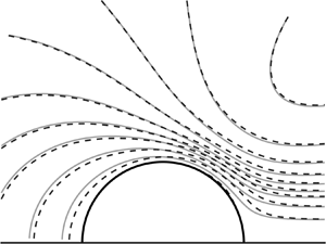
Figure 4. Pattern of the mean flow around a porous cylinder with (a) $K^\star = {0.1}$ and (b) $K^\star = {0.2}$ computed using an impedance boundary condition approach and following Power et al. (Reference Power, Miranda and Villamizar1984).

A proper boundary condition has to be applied to $\phi$ and $\boldsymbol {\psi }$ at the porous cylinder surface. For the former, the same approach as that followed in (3.9) is adopted, yielding

(3.10)\begin{equation} \frac{\partial \phi}{\partial r} = u_{r\infty} + K \phi \quad \text{at} \ r = {1}, \end{equation}

$u_{r\infty }$ being the radial component of the upstream velocity. For the latter, an assumption about the flow field inside the body is required. If the porous medium is homogeneous and the temperature variation is negligible, the internal flow may be represented as irrotational and be determined by the corresponding pressure related to the seepage velocity at the surface following Darcy's law (Bear Reference Bear1972). This is a consequence of the averaging procedure performed over the flow within the porous medium and agrees with the analysis carried out by Power et al. (Reference Power, Miranda and Villamizar1984). Indeed, although the flow inside each pore is viscous and, thus, rotational, the local rotations average out to an irrotational global motion. Therefore, the vortical term of the turbulent velocity can be assumed to be negligible at the surface and the boundary condition in (2.15) is employed also for the porous configuration.

3.3. Solution in terms of Fourier series

The expression of (2.28) and (2.29) in cylindrical coordinates yields

(3.11)\begin{equation} \left\lbrack\frac{\partial^2}{\partial r^2}+\frac{1}{r}\frac{\partial}{\partial r}+\frac{1}{r^2}\frac{\partial^2}{\partial \theta^2} - \kappa_3^2\right\rbrack \beta_{j} = {0} \end{equation}

and

(3.12)\begin{equation} \left.\begin{gathered} \left\lbrack \frac{\partial^2}{\partial r^2}+\frac{1}{r}\frac{\partial}{\partial r}+\frac{1}{r^2}\frac{\partial^2}{\partial \theta^2} -\frac{2}{r^2}\frac{\partial}{\partial\theta} -\left( \frac{1}{r^2}+\kappa_3^2 \right) \right\rbrack \tilde{\alpha}_{1j} ={-}\tilde{\varOmega}_{1j},\\ \left\lbrack \frac{\partial^2}{\partial r^2}+\frac{1}{r}\frac{\partial}{\partial r}+\frac{1}{r^2}\frac{\partial^2}{\partial \theta^2} -\frac{2}{r^2}\frac{\partial}{\partial\theta} -\left( \frac{1}{r^2}+\kappa_3^2 \right) \right\rbrack \tilde{\alpha}_{2j} ={-}\tilde{\varOmega}_{2j},\\ \left\lbrack\frac{\partial^2}{\partial r^2}+\frac{1}{r}\frac{\partial}{\partial r}+\frac{1}{r^2}\frac{\partial^2}{\partial \theta^2} - \kappa_3^2\right\rbrack \tilde{\alpha}_{3j} ={-}\tilde{\varOmega}_{3j}, \end{gathered}\right\}\end{equation}

where ${\tilde {\boldsymbol {\alpha }}}$ is obtained by a rotation in Euclidean space and is defined as

(3.13a–c)\begin{equation} \tilde{\alpha}_{1j} = \alpha_{1j}\cos{\theta}+\alpha_{2j}\sin{\theta}; \quad \tilde{\alpha}_{2j} ={-}\alpha_{1j}\sin{\theta}+\alpha_{2j}\cos{\theta}; \quad \tilde{\alpha}_{3j} = \alpha_{3j}, \end{equation}

whilst ${\tilde {\boldsymbol {\varOmega }}}$ is calculated from the distortion tensor in cylindrical coordinates,

(3.14)\begin{equation} \tilde{\varOmega}_{ij} = \left[{\tilde{\gamma}}_{ij} \exp({\textrm{i}(\kappa_1 \varDelta_t-\kappa_2 \varDelta_y)})-{\tilde{\gamma}}_{\infty,ij}\right] \exp({\textrm{i} r(\kappa_1 \cos{\theta}+\kappa_2 \sin{\theta})}) \end{equation}

with

(3.15a,b)\begin{equation} {\tilde{\gamma}}_{ij} = \begin{bmatrix} U_r & \sin{\theta} -\partial \varDelta_T/ r \partial \theta & {0}\\ U_\theta & \cos{\theta}+\partial \varDelta_T/\partial r & {0}\\ {0} & {0} & {1} \end{bmatrix}; \quad {\tilde{\gamma}}_{\infty,ij} = \begin{bmatrix} \cos{\theta} & \sin{\theta} & {0}\\ -\sin{\theta} & \cos{\theta} & {0}\\ {0} & {0} & {1} \end{bmatrix}. \end{equation}

The present expression for $\tilde {\boldsymbol {\gamma }}_{\boldsymbol {\infty }}$ represents the transpose of that reported by Hunt (Reference Hunt1973) in (4.7) of his paper.

One possible way to solve (3.11) and (3.12) is to avoid the dependence on $\theta$ and express $\boldsymbol {\beta }$, ${\tilde {\boldsymbol {\alpha }}}$ and ${\tilde {\boldsymbol {\varOmega }}}$ as Fourier series (Hunt Reference Hunt1973),

(3.16)\begin{equation} \left(\begin{array}{c} \beta_{j}\\ \tilde{{\alpha}}_{ij}\\ \tilde{{\varOmega}}_{ij} \end{array}\right) = \sum_{n=0}^{\infty} \left\{ \left(\begin{array}{c} \beta^{cn}_{j}\\ {\alpha}^{cn}_{ij}\\ {\varOmega}^{cn}_{ij} \end{array}\right) \left( r;\boldsymbol{\kappa} \right) \cos{n\theta} + \left(\begin{array}{c} \beta^{sn}_{j}\\ {\alpha}^{sn}_{ij}\\ {\varOmega}^{sn}_{ij} \end{array}\right) \left( r;\boldsymbol{\kappa} \right) \sin{n\theta} \right\}. \end{equation}

The computation of the Fourier coefficients implies that the aforementioned variables are defined all over the domain and that the boundary conditions at the cylinder surface are valid for $0 \leqslant \theta \leqslant 2{\rm \pi}$. This is made possible through the assumption of no-flow separation introduced in § 3.1.

By substituting (3.16) into (3.11) and (3.12), it follows that

(3.17)\begin{equation} \left\{ \frac{\partial^2}{\partial r^2}+\frac{1}{r}\frac{\partial}{\partial r} - \left( \frac{n^2}{r^2}+\kappa_3^2 \right) \right\} \left(\begin{array}{c} \beta_{j}^{cn}\\ \beta_{j}^{sn} \end{array}\right) = {0} \end{equation}

and

(3.18)\begin{equation} \left. \begin{gathered} \left\lbrack \frac{\partial^2}{\partial r^2}+\frac{1}{r}\frac{\partial}{\partial r} - \frac{1}{r^2} - \left( \frac{n^2}{r^2}+\kappa_3^2 \right) \right\rbrack \left(\begin{array}{c} \alpha_{1j}^{cn}\\ \alpha_{1j}^{sn} \end{array}\right) ={-}\left(\begin{array}{c} \varOmega_{1j}^{cn}\\ \varOmega_{1j}^{sn} \end{array}\right) + \frac{2n}{r^2} \left(\begin{array}{c} \alpha_{2j}^{sn}\\ -\alpha_{2j}^{cn} \end{array}\right), \\ \left\lbrack \frac{\partial^2}{\partial r^2}+\frac{1}{r}\frac{\partial}{\partial r} - \frac{1}{r^2} - \left( \frac{n^2}{r^2}+\kappa_3^2 \right) \right\rbrack \left(\begin{array}{c} \alpha_{2j}^{cn}\\ \alpha_{2j}^{sn} \end{array}\right) ={-}\left(\begin{array}{c} \varOmega_{2j}^{cn}\\ \varOmega_{2j}^{sn} \end{array}\right) - \frac{2n}{r^2} \left(\begin{array}{c} \alpha_{1j}^{sn}\\ -\alpha_{1j}^{cn} \end{array}\right), \\ \left\lbrack \frac{\partial^2}{\partial r^2}+\frac{1}{r}\frac{\partial}{\partial r} - \left( \frac{n^2}{r^2}+\kappa_3^2 \right) \right\rbrack \left(\begin{array}{c} \alpha_{3j}^{cn}\\ \alpha_{3j}^{sn} \end{array}\right) ={-}\left(\begin{array}{c} \varOmega_{3j}^{cn}\\ \varOmega_{3j}^{sn} \end{array}\right). \end{gathered}\right\} \end{equation}

The boundary conditions need to be converted into equations for the Fourier coefficients of $\boldsymbol {\beta }$ and ${\tilde {\boldsymbol {\alpha }}}$. For the former, it is possible to reformulate (2.15) and (3.10) considering the outward-pointing normal to the cylinder surface $\boldsymbol {n} = ( {1},{0},{0} )^\intercal$ as

(3.19)\begin{equation} \left. \begin{array}{ll@{}} \textit{Solid cylinder}{:} \quad \dfrac{\partial \beta_{j}}{\partial r} = \left( \cos{\theta},\sin{\theta},0 \right)^\intercal \exp({\textrm{i}( \kappa_1\cos{\theta}+\kappa_2\sin{\theta})}) & \text{at} \ r \!=\! {1}; \\ \textit{Porous cylinder}{:} \quad \dfrac{\partial \beta_{j}}{\partial r} \!=\! \left( \cos{\theta},\sin{\theta},0 \right)^\intercal \exp({\textrm{i}( \kappa_1\cos{\theta}+\kappa_2\sin{\theta})}) + K\beta_{j} & \text{at} \ r \!=\! {1}, \end{array}\right\} \end{equation}

which yields

(3.20)\begin{equation} \left.\begin{array}{ll@{}} \textit{Solid cylinder}{:} \quad \dfrac{\partial}{\partial r} \left(\begin{array}{c} \beta_{j}^{cn}\\ \beta_{j}^{sn} \end{array}\right) = \left(\begin{array}{c} G_{j}^{cn}\\ G_{j}^{sn} \end{array}\right) &\text{at} \ r = {1}; \\ \textit{Porous cylinder}{:} \quad \dfrac{\partial}{\partial r} \left(\begin{array}{c} \beta_{j}^{cn}\\ \beta_{j}^{sn} \end{array}\right) = \left(\begin{array}{c} G_{j}^{cn}\\ G_{j}^{sn} \end{array}\right) + K_\theta \left(\begin{array}{c} \beta_{j}^{cn}\\ \beta_{j}^{sn} \end{array}\right) &\text{at} \ r = {1}, \end{array}\right\}\end{equation}

where

(3.21)\begin{equation} \left(\begin{array}{c} G_{j}^{cn}\\ G_{j}^{sn} \end{array}\right) = \frac{I}{2{\rm \pi}} \int_0^{2{\rm \pi}} \left(\begin{array}{c} \cos{n\theta}\\ \sin{n\theta} \end{array}\right) \left( \cos{\theta},\sin{\theta},0 \right)^\intercal \exp({\textrm{i}( \kappa_1\cos{\theta}+ \kappa_2\sin{\theta})}) \,\textrm{d}\theta. \end{equation}

Here $I = {1}$ if $n = {0}$ and $I = {2}$ if $n > {0}$ as a consequence of the Fourier coefficients calculation. In this case, $K_\theta$ is the value of $K$ corresponding to the angular position of interest, which must be defined a priori. Furthermore, as $r \to \infty$, (2.16) implies that

(3.22)\begin{equation} \left(\begin{array}{c} \beta_{j}^{cn}\\ \beta_{j}^{sn} \end{array}\right) \to {0}. \end{equation}

For the latter, (2.17) at $r = {1}$ can be rewritten similarly to the previous case as

(3.23)\begin{equation} \left[ n \left(\begin{array}{c} \alpha_{3j}^{sn}\\ -\alpha_{3j}^{cn} \end{array}\right) - \textrm{i}\kappa_3 \left(\begin{array}{c} \alpha_{2j}^{cn}\\ -\alpha_{2j}^{sn} \end{array}\right) \right]_{r = {1}} = {0}. \end{equation}

Likewise, (2.18) for $x \to \infty$ leads to

(3.24)\begin{equation} \left.\begin{gathered} \frac{n}{r} \left(\begin{array}{c} \alpha_{3j}^{sn}\\ -\alpha_{3j}^{cn} \end{array}\right) - \textrm{i}\kappa_3 \left(\begin{array}{c} \alpha_{2j}^{cn}\\ \alpha_{2j}^{sn} \end{array}\right) = {0}, \\ \textrm{i}\kappa_3 \left(\begin{array}{c} \alpha_{1j}^{cn}\\ \alpha_{1j}^{sn} \end{array}\right) - \frac{\partial}{r} \left(\begin{array}{c} \alpha_{3j}^{cn}\\ \alpha_{3j}^{sn} \end{array}\right) = {0}, \\ \frac{1}{r} \frac{\partial}{r} \left\{ r \left( \begin{array}{c} \alpha_{2j}^{cn}\\ -\alpha_{2j}^{sn} \end{array}\right) \right\} - \frac{n}{r} \left(\begin{array}{c} \alpha_{1j}^{sn}\\ -\alpha_{1j}^{cn} \end{array}\right) = {0}, \end{gathered}\right\}\end{equation}

whilst the application of the gauge condition (2.19) for $r = {1}$ and as $x \to \infty$ yields

(3.25)\begin{equation} \frac{1}{r}\frac{\partial}{\partial r} \left\{ r \left(\begin{array}{c} \alpha_{1j}^{cn}\\ \alpha_{1j}^{sn} \end{array}\right) \right\} + \frac{n}{r} \left(\begin{array}{c} \alpha_{2j}^{sn}\\ -\alpha_{2j}^{cn} \end{array}\right) + \textrm{i}\kappa_3 \left(\begin{array}{c} \alpha_{3j}^{cn}\\ \alpha_{3j}^{sn} \end{array}\right) = {0}. \end{equation}

As discussed in § 3.2, the present equations have to be satisfied for both cylinder configurations.

Equations (3.17) and (3.18) can be solved by means of the modified Bessel functions and the method of variation of parameters. The detailed derivations are reported in appendix A. Once the different components of $\boldsymbol {\beta }$ and ${\tilde {\boldsymbol {\alpha }}}$ are obtained, $\boldsymbol{\mathsf{M}}$ is found in Cartesian coordinates. In this case, $\boldsymbol {{\alpha }}$ is computed from (3.13a–c) by inverting the rotation matrix.

3.4. Turbulence-distortion mechanisms

A bluff body affects the incoming turbulent flow in two ways: (i) through the distortion of the vorticity field that alters the mean-velocity field both around and upstream of the body, and (ii) through the pressure exerted by the body, which blocks, partially or completely, the wall-normal turbulence velocity fluctuations. The influence of the vorticity distortion on the evolution of the velocity fluctuations is typically negligible if the integral length scale of the turbulent flow, $L_x$, is much higher than the characteristic dimension of the cylinder, $a$. In contrast, the body always exerts a reaction pressure field on the flow, regardless of the scales being considered.

The Helmholtz decomposition expressed by (2.12) is instrumental in investigating the two turbulence-distortion mechanisms. Indeed, the first effect is linked to the component $\boldsymbol {\nabla } \boldsymbol {\times } \boldsymbol {\psi }$ and mostly alters the velocity of the small-scale eddies ($k\gg 1$), whilst the second one is associated with the component $\boldsymbol {\nabla } \phi$ and mainly impacts the velocity of the large-scale eddies ($k\ll 1$). The same decomposition is applied to the velocity distortion tensor, which, from (2.33), can be seen as the sum of (i) a term $\boldsymbol{\mathsf{M}}^{(\mathrm{s})}$ that is related to the blocking of velocity fluctuations by the pressure of the body, (ii) a term $\boldsymbol{\mathsf{M}}^{(\mathrm{d})}$ that depends on the distortion of vorticity by the mean flow and (iii) a term $\boldsymbol{\mathsf{M}}^{({\infty })}$ that is fully determined by the upstream conditions. In § 4 the influence of porosity on the turbulence distortion will be analysed in terms of these quantities.

3.5. Computational methodology

The distortion tensor $\boldsymbol{\mathsf{M}}$ is calculated following the approach proposed by Hunt (Reference Hunt1973) but with a finer discretization of the calculation domain, which has proved to yield a better accuracy. A total of ${380}$ values of $r$ from $r = {1.05}$ to $r = {10}$ and ${50}$ angular positions from $\theta = {5}{\rm \pi} /{6}$ to $\theta = {\rm \pi}$ are considered, with a resolution ranging from ${0.01}$ near the stagnation point to ${0.025}$ for $r > {3}$ and ${0.05}$ for $r > {5}$ for the radial coordinate and a uniform resolution of about ${\rm \pi} /300$ for the angular one. Therefore, the resulting grid consists of a total of 16 500 points and is depicted in figure 5 for ${0} < r < {5}$.

Figure 5. Domain for the computation of the velocity distortion tensor. The dots define the calculation locations, whilst the solid lines represent the mean-flow pattern for the case of a solid cylinder.

The wavenumber domain used for the integration of $\boldsymbol{\mathsf{M}}$ according to (2.34) and (2.35) must be truncated in order to ensure that all wavenumbers can be adequately represented on the grid shown in figure 5. The maximum value of the non-dimensional streamwise wavenumber $\kappa _1$ is set to ${5}$. In addition, instabilities in the energy spectra occur when $\kappa _1, \kappa _2 > {1}$ and $\kappa _3 \rightarrow {0}$. Hence, $\boldsymbol{\mathsf{M}}$ is only calculated for normalised wavenumbers greater than ${0.001}$. Convergence tests showed that ${25}$ values for each component are sufficient, leading to a total of 15 625 points.

All the functions are calculated by means of routines implemented in the commercial software MATLAB® by MathWorks. The integrations are performed through the Simpson's rule, whilst the modified Bessel functions are computed by means of standard subroutines with a tolerance of the order of $2\times 10^{-16}$. The Fourier series approach in (3.16) requires $\boldsymbol {\varOmega }$ to be estimated for ${0} < \theta < {\rm \pi}$ in order to determine $\boldsymbol {{\varOmega }}^{cn}$ and $\boldsymbol {{\varOmega }}^{sn}$. The calculation is performed considering ${1000}$ values of $\theta$ with regular spacings of ${\rm \pi} /500$ and a $\delta \theta$ of ${\rm \pi} /100$. For the Fourier series decomposition, $n_{{max}}$ is set to ${100}$ in order to ensure an accurate reconstruction of the original function. The convergence is evaluated by estimating the ratio $\lambda _c$ of the modulus of the largest $\varOmega _{11}^{cn}$ in the series to the modulus of the last term. Values of $\lambda _c$, evaluated at $r = {1.01}$ and $r = {3.6}$ for different wavenumbers, are reported in table 1 for $K^\star = {0}$ (solid cylinder) and $K^\star = {0.2}$ (porous cylinder). The table also shows the values of the largest $\varOmega _{11}^{cn}$ and the value of $n$ at which $\varOmega _{11}^{cn}$ is maximum. The chosen locations and the presented parameters allow for a direct comparison with the results listed in table 3 of the original paper of Hunt (Reference Hunt1973).

Table 1. Properties of the Fourier series of $\varOmega _{11}^{cn}$ for a solid ($K^\star = {0}$) and porous ($K^\star = {0.2}$) cylinder. Here $( \varOmega _{11}^{cn} )_{{max}}$ is the largest term of the series, $n_{{max}}$ is the Fourier mode at which $\varOmega _{11}^{cn}$ is maximum and $\lambda _c = |(\varOmega _{11}^{cn})_{{max}}|/|\varOmega _{11}^{c100}|$.

Conclusions similar to those of Hunt can be drawn in this case. For both cylinders, $\lambda _c$ decreases as the wavenumber increases as a consequence of the more rapid variations in $\varOmega _{11}^{cn}$ occurring over smaller distances. Likewise, the convergence is slower for higher values of $r$ due to the larger distance in the angular direction and leads to more significant inaccuracies in the reconstruction of the function. However, the values of $\lambda _c$ are notably higher than those computed by Hunt (Reference Hunt1973) for every considered case and this justifies the choice of an increased $n$, especially for $\kappa _1 = \kappa _2 = {10}$. Furthermore, the comparison with the porous case exhibits two different trends. At $r = {1.01}$, the convergence for $K^\star = {0.2}$ is considerably slower than that for the corresponding solid case due to the additional terms in the velocity components of (3.7). Therefore, more Fourier series modes would be required to reach the same accuracy in the reconstruction of $\varOmega _{11}^{cn}$ as in the case of $K^\star = {0}$. Yet, at least one order of magnitude of difference is seen between $|( \varOmega _{11}^{cn} )_{{max}}|$ and $|\varOmega _{11}^{c100}|$ in the most critical case at $\kappa _1 = \kappa _2 = {10}$, allowing for a satisfactory convergence in the computation of the turbulent flow near the porous cylinder for high wavenumbers. At $r = {3.60}$, the deviation between the solid and porous case is negligible, hinting at an effect of porosity localised in the proximity of the body surface. This trend is confirmed by the lines of constant $\varDelta _T$ and by the results of the incident velocity spectra presented in § 4.2.

3.6. Algorithm validation

The validation of the adopted methodology is carried out by comparing the RDT one-dimensional velocity spectra with the experimental results of Britter et al. (Reference Britter, Hunt and Mumford1979), who performed velocity measurements on a circular cylinder placed downstream of planar square grids that produced approximately homogeneous isotropic turbulence with different length scales. The spectra are presented using the following scaling in order to avoid the dependence on the parameter $L_x/a$,

(3.26a,b)\begin{equation} \boldsymbol{\hat{\varTheta}}(x,y;\boldsymbol{\hat{\kappa}}) = \frac{a}{L_x} \, \boldsymbol{\varTheta}(x,y;\boldsymbol{\kappa}); \quad \hat{\boldsymbol{\kappa}} = \frac{L_x}{a} \boldsymbol{\kappa}. \end{equation}

With this notation, the transition between the energy-containing eddies and the inertial subrange occurs at $\hat {\kappa }_1 \approx {1}$. Furthermore, it indicates that the lower the ratio of $L_x/a$ that is considered is, the higher the maximum $\kappa _1$ that must be computed to have an accurate description of the velocity field will be. This provides a limitation on the turbulence scales calculated in the present analysis, which focuses on the case $L_x > a$. It is important to point out that $\hat {\kappa }_1$ corresponds to a normalised frequency made dimensionless by $L_x$ and $\bar {u}_{\infty }$ throughout the flow. It effectively represents a convective wavenumber only in the undisturbed flow, whilst near the cylinder it would be considered as a true convective wavenumber if it were normalised with the local mean velocity.

The comparison between the RDT calculations for an impermeable cylinder and the data taken at $x = {-4}$ and $x = {-1.2}$ along the stagnation streamline is shown in figure 6. These refer to three values of $L_x/a$, namely $L_x/a = {9.09}$, $L_x/a = {2.86}$ and $L_x/a = {1.56}$. The results are supplemented by the expressions computed through the von Kármán model in (2.36) that are meant to approximate the upstream spectra. The first observation is that the measured undisturbed RDT spectra at $x = {-4}$ almost coincide with the von Kármán model over the whole frequency range. This is related to the fact that in the considered wavenumber range $\boldsymbol{\mathsf{M}}$ reduces to the identity matrix at a location sufficiently far from the cylinder surface.

Figure 6. Comparison between the RDT spectra of the streamwise (a,c,e) and upwash (b,d,f) velocity components and the measurements of Britter et al. (Reference Britter, Hunt and Mumford1979) at two locations along the stagnation streamline for (a,b) $L_x/a = {9.09}$, (c,d) $L_x/a = {2.86}$ and (e,f) $L_x/a = {1.56}$. The undisturbed spectra computed with the von Kármán model are also reported.

Secondly, while the agreement between the experimental results and the von Kármán model is satisfactory for the streamwise component everywhere, the spectra of the upwash velocity component exhibit a deviation in the low-frequency range. The present trend has been already pointed out by Britter et al. (Reference Britter, Hunt and Mumford1979) and Jackson, Graham & Maull (Reference Jackson, Graham and Maull1973) and is due to the finite ratio of the wind-tunnel width to the grid mesh size. However, the effect of the aspect ratio is mainly significant in the low-frequency range and the von Kármán model agrees with the measurements elsewhere. Furthermore, at the most upstream location, the two velocity components exhibit opposite evolutions for all the considered values of $L_x/a$. The streamwise velocity decreases, whereas the upwash component increases. This is a consequence of the energy transfer that occurs between $\hat {\varTheta }_{11}$ and $\hat {\varTheta }_{22}$ due to the blocking effect of the impermeable body. The present trend is more pronounced for larger turbulence scales due to the dominance of this turbulence-distortion mechanism for $k \gg {1}$.

Comparing the RDT calculations with the experimental results leads to interesting conclusions. For the streamwise velocity component, the agreement is generally better for larger values of $L_x/a$, with the distorted spectra that show a comparable $\Delta \hat {\varTheta }_{11}$ with the upstream ones at lower $\hat {\kappa }_1$ and start converging at higher $\hat {\kappa }_1$. Yet, the overlapping occurs at lower frequencies for the experimental results than for the RDT prediction. The magnitude of this deviation increases with the decreasing value of $L_x/a$ and can be attributed to the truncation of the wavenumber domain at $\boldsymbol {\kappa } = [{5},{5},{5}]$. This affects the integration in (2.34) and yields an energy deficit in the disturbed spectra that modifies the slope with which they decay. Moreover, the deficit decreases for larger turbulence scales with respect to the lower ones since higher values of $L_x/a$ correspond to augmented normalised frequencies according to (3.26a,b). For the upwash velocity components, only a qualitative comparison can be carried out due to the effect of the wind-tunnel width. Likewise, the RDT calculations and the measurements feature analogous trends in terms of $\Delta \hat {\varTheta }_{22}$ and frequency-dependence behaviour, with a better correspondence for larger values of $L_x/a$. In this case, the spectra at $x = {-1.2}$ exhibit lower values than the upstream ones at higher frequencies and the trade-off point moves towards lower $\hat {\kappa }_1$ with the decreasing turbulence scale.

4.1. Mean-flow deflection

Porosity alters the mean-flow field near the cylinder surface due to the flow penetration. Figures 4(a) and 4(b) illustrate the mean-flow streamlines computed by the velocity potential of (3.5) and by the impedance boundary condition in (3.9) for $K^\star = {0.1}$ and $K^\star = {0.2}$, respectively. For both cases, the two approaches provide approximately the same flow pattern for $x < {0}$, whereas increasing deviations occur for $x > {0}$. In particular, the streamline closest to the body exhibits the most significant difference between the two methods, probably due to the limitations of the impedance boundary condition approach in effectively modelling the internal Darcy's flow in the rear part of body. Moreover, the deviations increase with increasing $K^\star$ since the regularisation procedure extends over a wider range of $\theta$. In any case, the present region of interest is centred around the cylinder stagnation point, where the agreement between the two methods is satisfactory.

The altered deflection of the mean flow in the presence of porosity has an impact on $\boldsymbol {\mathbb {\gamma }}$ and thereby on $\boldsymbol {\omega }$. Indeed, the second term that appears in the mean-velocity field expressed by (3.7) affects $\gamma _{11}$ and $\gamma _{21}$, whereas the formulation of $\varDelta _T$ for the porous case modifies $\gamma _{12}$ and $\gamma _{22}$. This last aspect is made evident in figures 7(a) and 7(b), which display lines of constant $\varDelta _T$ for a solid and porous cylinder with $K^\star = {0.1}$ and $K^\star = {0.2}$, respectively. In fact, the possibility of the incident velocity penetrating the inner volume leads to a reduction in the time taken for a fluid particle to reach a point in the vicinity of the body surface, which constitutes a reduced geometrical discontinuity with respect to a solid wall. The deviation in $\varDelta _T$ is more evident in the proximity of the stagnation region and reflects the trend of $K$ in figure 3 that features a local minimum at $\theta = {\rm \pi}$. As expected, the effect of porosity is more pronounced in terms of amplitude and extension in the case of $K^\star = {0.2}$. In addition, the results for the solid cylinder closely reproduce those shown in figure 4 in Hunt (Reference Hunt1973) and validate the implementation of this function.

Figure 7. Lines of constant $\varDelta _T$ for a solid ($K^\star = {0}$) and porous cylinder characterised by (a) $K^\star = {0.1}$ and (b) $K^\star = {0.2}$.

4.2. One-dimensional spectra

The modifications in the one-dimensional velocity spectra due to the presence of porosity exhibit two opposite trends. Figure 8 illustrates the spectra of the streamwise and upwash component of the turbulent velocity computed at $x = {-1.1}$ and $\theta = {\rm \pi}$ (stagnation streamline) for $L_x/a = {9.09}$, $L_x/a = {2.86}$ and $L_x/a = {1.56}$. These are compared with the undistorted spectra calculated at $x = {-5}$, which coincide for all the cylinder configurations. The velocity is made dimensionless by $u^{\prime }_{\infty }$, whilst the results are presented on a logarithmic scale in order to better visualise the deviations between the solid and porous cases.

Figure 8. Solid and porous ($K^{\star } = {0.1}$ and $K^{\star } = {0.2}$) spectra of the streamwise (a,c,e) and upwash (b,d,f) velocity components computed at $x = {-1.1}$ and $\theta = {\rm \pi}$ for (a,b) $L_x/a = {9.09}$, (c,d) $L_x/a = {2.86}$ and (e,f) $L_x/a = {1.56}$. The undisturbed spectra are shown as opaque lines.

The influence of porosity is seen to take place close to the cylinder surface and is more significant for larger turbulence scales, as exemplified by the case $L_x/a = {9.09}$. The decrease in the streamwise component (figure 8a) is attenuated in the porous cases and the effect is mostly confined to low normalised frequencies. Similarly, the upwash component (figure 8b) exhibits lower values in the same range. As expected, the deviation is higher for the case with the larger $K^{\star }$. However, at high normalised frequencies, the porous spectra start diverging from the solid one and this occurs at the intersection point with the undisturbed spectra. Here $K^{\star }$ does not affect the normalised frequency at which the deviation starts but alters the slope with which the spectra diverge from the solid configuration.

Similar conclusions can be drawn for $L_x/a = {2.86}$, although, in this case, the impact of porosity is less pronounced in the low-frequency range for both streamwise (figure 8c) and upwash (figure 8d) velocity components. As already pointed out in § 3.6, the amplification in $\hat {\varTheta }_{22}$ due to the energy transfer is less than for larger turbulent scales and this yields a shift of the above-mentioned intersection point towards lower normalised frequencies. Likewise, the slope gets closer to that of the undisturbed case for frequencies beyond the intersection point and the deviation is more significant for $K^{\star } = {0.2}$ than for $K^{\star } = {0.1}$. The trends discussed above about the effect of reducing the turbulence scales are still observed when further decreasing $L_x/a$ from ${2.86}$ to ${1.56}$, as seen in figures 8(e) and 8(f).

Additional remarks can be made when the velocity spectra are evaluated at an angular position slightly away from the stagnation point. Figure 9 presents the results of the RDT calculations performed at $\theta = 5{\rm \pi} /6$. The first observation is that the attenuation in $\hat {\varTheta }_{11}$ from the upstream values is less than that at $\theta = {\rm \pi}$, thereby mimicking the behaviour of the mean streamwise velocity. The second observation is that the impact of porosity is reduced in the low-frequency range as a consequence of the trend of $K$ illustrated in figure 3(a), which features values of the dimensionless porous parameter closer to zero at $\theta = 5{\rm \pi} /6$. Interestingly, while for the upwash velocity component the same conclusions as for the case at $\theta = {\rm \pi}$ are drawn for the dependence of the energy attenuation on the turbulence scale, a different trend is observed for the streamwise component. Indeed, no substantial difference between the solid and porous cases can be appreciated for $\hat {\varTheta }_{11}$ at $L_x/a = {9.09}$, whereas increasing deviations occur for $L_x/a = {2.86}$ and $L_x/a = {1.56}$. The third observation is that the high-frequency deviation for the upwash velocity spectra still occurs at the intersection point with the undisturbed ones but, notably, this phenomenon extends also to the streamwise velocity spectra, which start diverging from normalised frequencies that reduce with decreasing $L_x/a$. Likewise, the divergence is more pronounced for the larger value of $K^{\star }$.

Figure 9. Solid and porous ($K^{\star } = {0.1}$ and $K^{\star } = {0.2}$) spectra of the streamwise (a,c,e) and upwash (b,d,f) velocity components computed at $x = {-1.1}$ and $\theta = 5{\rm \pi} /6$ for (a,b) $L_x/a = {9.09}$, (c,d) $L_x/a = {2.86}$ and (e,f) $L_x/a = {1.56}$. The undisturbed spectra are shown as opaque lines.

The trends seen in figures 8 and 9 may be analysed in terms of the velocity distortion tensors $\boldsymbol{\mathsf{M}}^{(\mathrm{s})}$ and $\boldsymbol{\mathsf{M}}^{(\mathrm{d})}$. When the scale of the incoming turbulence is large compared with the characteristic length of the body, the possibility of the potential component of the incident velocity penetrating the cylinder's inner volume alters the blocking effect of the surface and affects $\boldsymbol{\mathsf{M}}^{(\mathrm{s})}$. This phenomenon has an impact mostly on the low-frequency range of the spectra and results in a damping of the turbulence distortion and a reduction in the change of the streamwise and upwash velocity fluctuations near the stagnation point. When $L_x \approx a$ or, in general, at high normalised frequencies, the effect of porosity on $\boldsymbol{\mathsf{M}}^{(\mathrm{s})}$ is limited and does not yield a significant alteration in the turbulent velocity.

Nevertheless, the modification of the mean flow due to the porous surface indirectly modifies $\boldsymbol{\mathsf{M}}^{(\mathrm{d})}$ and is responsible for the high-frequency deviation in the one-dimensional spectra occurring at the intersection point with the undisturbed spectra. This trend can be qualitatively explained by considering the evolution of a fluid line element approaching the cylinder along the stagnation streamline. As this is advected towards the body by the mean flow, its lengths $\textrm {d}l_1$, $\textrm {d}l_2$ and $\textrm {d}l_3$ undergo a change and so do the different components of the vorticity associated with the element (Hunt Reference Hunt1973). Indeed, the vorticity field is solenoidal, i.e. $\boldsymbol{\nabla \cdot\omega} = 0$: a compression of the fluid element in one direction results in an increase in $\boldsymbol{\omega}$ in the other directions. In particular, $\textrm {d}l_1$ is compressed and $\textrm {d}l_2$ is stretched due to the blockage effect of the obstacle, leading to an attenuation of $\omega _1$ and an amplification of $\omega _2$, respectively, whereas no modification in $\textrm {d}l_3$ and, therefore, in $\omega _3$ is expected. The mitigation of $\omega _1$ and the invariance of $\omega _3$ will, in turn, induce a reduction in the upwash component of the turbulent velocity that is localised in the high-frequency range of the spectrum, as mentioned in § 3.4. The present mechanism is weakened for the case of a porous cylinder and the decrease in $\varTheta _{22}$ is lesser than that for the solid configuration. This is at the basis of the high-frequency deviation in the one-dimensional spectra.

Figure 10 illustrates those effects through the evolution of $|\boldsymbol{\mathsf{M}}^{(\mathrm{s})}_{11}|$, $|\boldsymbol{\mathsf{M}}^{(\mathrm{d})}_{11}|$, $|\boldsymbol{\mathsf{M}}^{(\mathrm{s})}_{22}|$ and $|\boldsymbol{\mathsf{M}}^{(\mathrm{d})}_{22}|$ along the stagnation streamline for a solid and porous cylinder characterised by $K^{\star } = {0.2}$. Two different wavenumber vectors are computed in this case: $\boldsymbol {\kappa } = [{0.1},{0.1},{0.1}]$ and $\boldsymbol {\kappa } = [{1},{1},{1}]$. For the former (figure 10a,b), the distortion generated by $\boldsymbol{\mathsf{M}}^{(\mathrm{d})}$ can be considered negligible and the porous surface has a substantial influence on $\boldsymbol{\mathsf{M}}^{(\mathrm{s})}$, the magnitude of which is reduced in absolute terms. For the latter (figure 10c,d), the two turbulence-distortion mechanisms feature comparable values near the body and porosity alters both $\boldsymbol{\mathsf{M}}^{(\mathrm{s})}$ (yet, with less impact than for the lowest wavenumber amplitude) and $\boldsymbol{\mathsf{M}}^{(\mathrm{d})}$.

Figure 10. Evolution of different components of $\boldsymbol{\mathsf{M}}$ along the stagnation streamline computed for (a,b) $\kappa _1 = \kappa _2 = \kappa _3 = {0.1}$ and (c,d) $\kappa _1 = \kappa _2 = \kappa _3 = {1}$ and for a solid ($K^{\star } = {0}$) and porous ($K^{\star } = {0.2}$) cylinder.

4.3. Variance along the stagnation streamline

The integration of the turbulent-velocity spectra of figure 8 at each position of the domain along the stagnation streamline allows for the evaluation of the variance of the turbulent-velocity components. Figure 11 illustrates the square root of the normalised variance of the streamwise and upwash turbulent-velocity components for the solid and porous cylinders computed for different values of $L_x/a$. In addition, the asymptotic limit for $L_x/a \rightarrow \infty$ is plotted. Indeed, a closed-form expression of the RDT for this case describing the fluctuating-velocity field around the body can be derived given the mean-velocity field and its rate of change due to small alterations in the direction of the incident flow. Following Bearman (Reference Bearman1972), the r.m.s. of the turbulent-velocity components are then given by

(4.1) \begin{equation} \left.\begin{gathered} \sqrt{\overline{u_{1}^2}} = {\mathsf{M}}^{(0)}_{11} \sqrt{\overline{u_{\infty,1}^2}} +{\mathsf{M}}^{(0)}_{12} \sqrt{\overline{u_{\infty,2}^2}}, \\ \sqrt{\overline{u_{2}^2}} = {\mathsf{M}}^{(0)}_{21} \sqrt{\overline{u_{\infty,1}^2}} + {\mathsf{M}}^{(0)}_{22} \sqrt{\overline{u_{\infty,2}^2}}, \end{gathered}\right\} \end{equation}

with

(4.2)\begin{equation} {\mathsf{M}}^{(0)}_{ij} =\begin{bmatrix} 1-\dfrac{x^2-y^2}{\left(x^2+y^2\right)^2} & \dfrac{2xy}{\left(x^2+y^2\right)^2} \\ \dfrac{-2xy}{\left(x^2+y^2\right)^2} & 1+\dfrac{x^2-y^2}{\left(x^2+y^2\right)^2} \end{bmatrix}. \end{equation}

Along the stagnation streamline, (4.1) and (4.2) reduce to

(4.3a,b)\begin{equation} \sqrt{\frac{\overline{u_1^2}}{\overline{u_{\infty,1}^2}}} = \left(1-\frac{1}{x^2}\right); \quad \sqrt{\frac{\overline{u_2^2}}{\overline{u_{\infty,2}^2}}} = \left(1+\frac{1}{x^2}\right). \end{equation}

Figure 11. Solid and porous ($K^{\star } = {0.1}$ and $K^{\star } = {0.2}$) variances of the streamwise (a,c,e) and upwash (b,d,f) velocity components computed along the stagnation streamline for (a,b) $L_x/a = {9.09}$, (c,d) $L_x/a = {2.86}$ and (e,f) $L_x/a = {1.56}$, and normalised by their upstream values. The asymptotic case for $L_x/a \rightarrow \infty$ is also reported.

The normalised variances for $L_x/a = {9.09}$ (figure 11a,b) are effectively approximated by the asymptotic analysis for every configuration. Yet, the porous cases exhibit increasingly higher values in the streamwise component and increasingly lower values in the upwash component when the stagnation point is approached, reflecting the trend observed in the one-dimensional spectra in § 4.2. In particular, the maximum deviation in $\overline {u_1^2}$ between solid and porous configurations occurs at the location nearest to the cylinder and amounts to approximately ${7.5}\,\%$ for $K^{\star } = {0.1}$ and 15 % for $K^{\star } = {0.2}$, whereas that in $\overline {u_2^2}$ amounts to approximately 5 % for $K^{\star } = {0.1}$ and 10 % for $K^{\star } = {0.2}$. Furthermore, the reduction in the upwash velocity component is a result of the partial compensation between the low-frequency decrease and the high-frequency increase due to porosity illustrated in figures 8 and 9. This, in turn, can potentially trigger a mitigation of the TIN mechanism, as will be shown in the NACA-0024 aerofoil case described in § 4.4.

At $L_x/a = {2.86}$ (figure 11c,d), the normalised variances deviate farther away from the asymptotic behaviour, whilst the effect of porosity is reduced. Indeed, the maximum deviation in $\overline {u_1^2}$ decreases to about 6 % and 12.5 % for $K^{\star } = {0.1}$ and $K^{\star } = {0.2}$, respectively, whereas that in $\overline {u_2^2}$ decreases to about 3 % and 5.5 % for $K^{\star } = {0.1}$ and $K^{\star } = {0.2}$, respectively. The present trend is further accentuated at $L_x/a = {1.56}$ (figure 11e,f), for which the streamwise velocity component remains unaltered up to $x = {-2}$ and then drops to zero in the vicinity of the cylinder surface. Only marginal differences can be observed between the solid and both porous configurations in this case, amounting to approximately 5 % and 10 % for $K^{\star } = {0.1}$ and $K^{\star } = {0.2}$, respectively. Conversely, the normalised variances of the upwash velocity component almost coincide for all the considered cases as a result of the compensation between the two opposite turbulence-distortion mechanisms that occur when $L_x \approx a$. Moreover, the decreased amplification in the one-dimensional spectra for the solid configuration, already discussed in § 4.2, is reflected in lower $\overline {u_2^2}$ near the cylinder surface. This is in agreement with the asymptotic analysis for small-scale turbulence (Batchelor & Proudman Reference Batchelor and Proudman1954; Bearman Reference Bearman1972; Hunt Reference Hunt1973), which shows that, for $L_x \ll a$, the upwash component of the turbulent velocity undergoes reduction when the stagnation point is approached due to the fast pile-up of vortex lines of opposite signs occurring at high wavenumbers.

4.4. Application case: porous NACA-0024 aerofoil

The modelling of the porous NACA-0024 profile case introduced in § 1 is based on the design that has been considered for the integration of the melamine foam in its inner volume. The characterisation of the parameters defining the porous medium is described in Satcunathan et al. (Reference Satcunathan, Zamponi, Meinke, Van de Wyer, Schram and Schröder2019). The aerofoil under consideration possesses a chord of 0.157 m and a span of 0.2 m, and is immersed in a flow characterised by a free-stream flow speed of $30\ \textrm {m}\ \textrm {s}^{-1}$ and by a ratio of $L_x$ to the leading-edge radius $r_{LE}$ of ${4.2}$. It features a permeable hard-plastic exo-skeleton that incorporates the porous material and ensures the integrity of the aerofoil shape. This component is coated with a metallic wire mesh that reduces the surface roughness, whilst an impermeable middle-plane prevents the cross-flow between the two sides of the NACA-0024 profile. However, its extent does not cover the first 6.4 % of the chord, corresponding to one leading-edge radius, in order to allow for flow penetration at the stagnation point. A sketch of the porous aerofoil design is depicted in figure 12(a). One of the conclusions drawn by the authors is that the presence of the permeable exo-skeleton allows for an alteration of the velocity fluctuations and has a limited impact on the mean-velocity field in the stagnation region, preserving the potential effect of the body. This evidence is supported by the results of the static pressure measurements on the surface of the porous aerofoil shown in figure 10 in Zamponi et al. (Reference Zamponi, Satcunanathan, Moreau, Ragni, Meinke, Schröder and Schram2020).

Figure 12. (a) Representation of the porous NACA-0024 profile featuring the solid middle-plane that prevents the cross-flow between pressure and suction side, the hard-plastic exo-skeleton that preserves the aerofoil shape integrity and the metallic wire mesh that ensures the desired surface roughness. (b) Acoustic beamforming results exhibiting the sound pressure levels radiated by a solid and porous aerofoil configuration expressed in one-third octave bands. The wavenumber vector is made dimensionless by the aerofoil leading-edge radius. Credits: Zamponi et al. (Reference Zamponi, Satcunanathan, Moreau, Ragni, Meinke, Schröder and Schram2020).

In view of the above, the porous aerofoil may be modelled by imposing the same deviation in mean flow produced by the solid configuration and applying the impedance boundary condition (3.10). In this case, the porous parameter is tuned considering (i) the static permeability of the melamine foam, $k_0 = 1.410\times 10^{-9}\ \textrm {m}^{2}$, which is assumed to be homogeneous; (ii) the leading-edge radius, $a = r_{LE} = 0.01\ \textrm {m}$; and (iii) the mean-flow speed downstream of the cylindrical rod, $U_{\infty } = 23\ \textrm {m}\ \textrm {s}^{-1}$, resulting in $K^{\star } \approx {0.22}$. This value still makes it possible to neglect the higher-order terms in (3.10).

Figure 13(a) depicts the one-dimensional spectra of the upwash velocity component computed at $x = {-1.05}$ for $L_x/a = {4.2}$. These are compared with the power spectra of the corresponding turbulent-velocity component for the solid and porous aerofoil configuration. The spectra exhibit a relative agreement with the measurements in the frequency range at which porosity has an impact, highlighting the key role played by the altered blocking effect of the porous aerofoil in the low-frequency mitigation of $\hat {\varTheta }_{22}$. A reduction of approximately 1.5 dB can be observed up to about the transition between the energy-containing eddies and the inertial subrange at $\hat {\kappa }_1 \approx {1}$ in the RDT calculations. Beyond this wavenumber, the solid and porous spectra start gradually converging and the influence of porosity on the flow field diminishes.

Figure 13. (a) Solid and porous ($K^{\star } = {0.22}$) spectra of the upwash velocity component computed at $x = {-1.05}$ for $L_x/a = {4.2}$. The RDT calculations are compared with the hot-wire anemometry measurements performed by Zamponi et al. (Reference Zamponi, Satcunanathan, Moreau, Ragni, Meinke, Schröder and Schram2020). (b) Solid and porous ($K^{\star } = {0.22}$) normalised variances of the streamwise and upwash velocity components computed along the stagnation streamline for $L_x/a = {4.2}$.

The experimental results feature the same trend and the same $\Delta \hat {\varTheta }_{22}$ in the low-frequency range, although the turbulence downstream of the rod does not meet the condition of homogeneity and isotropy assumed by the theory. This suggests that the relative alterations in turbulence distortion due to porosity are independent of the nature of the incident flow. However, deviations occur in correspondence with the frequency peak related to the vortex shedding in the wake of the upstream circular rod, which is not modelled in the present case. Interestingly, the reduction in $\hat {\varTheta }_{22}$ around the aforementioned peak is more pronounced in the measurements, probably due to the better hydrodynamic absorption of the large turbulent eddies shed by the rod. Since vortex shedding mostly affects the upwash turbulent-velocity component, a better agreement is expected for the streamwise component in general. In addition, the RDT calculations approximate well the experimental results in the inertial subrange but exhibit an underprediction at high normalised frequencies. This could be related to the truncation of the wavenumber domain that has already been addressed in § 3.6. An extension of the computed wavenumber range would most likely lead to a more accurate description of the turbulent-velocity field in this region.

Figure 13(b) illustrates the variance of turbulent velocities computed along the stagnation streamline for both solid and porous cylinder configurations. Trends analogous to the case $L_x/a = {9.09}$ can be observed in this instance, even though the mitigation of the velocity fluctuations is stronger than the one that would be present without the exo-skeleton due to the absence of the high-frequency amplification previously discussed. In particular, both an increase in $\overline {u_1^2}$ and decrease in $\overline {u_2^2}$ amount to approximately 12 %. These results significantly extend the preliminary analysis conducted by Zamponi et al. (Reference Zamponi, Satcunanathan, Moreau, Ragni, Meinke, Schröder and Schram2020), which was based on the RDT asymptotic solution in (4.1). Likewise, the predictions qualitatively agree with the conclusions drawn by the investigation of the measured turbulent-velocity fluctuations (figure 11 in Zamponi et al. Reference Zamponi, Satcunanathan, Moreau, Ragni, Meinke, Schröder and Schram2020) and of the large-eddy simulations (figures 13(b) and 14 in Zamponi et al. Reference Zamponi, Satcunanathan, Moreau, Ragni, Meinke, Schröder and Schram2020). Nevertheless, the porous RDT model described in this work is not suitable for providing a quantitative estimation of the evolution of the r.m.s. of the velocity fluctuations along the stagnation streamline in the case of a wing profile. Indeed, the potential flow around a circular cylinder starts to increasingly differ from that around the aerofoil moving away from the leading edge and the inflow distortion is no longer representative of the considered test case. The use of the actual potential solution for the wing profile could possibly tackle this problem.

The results detailed above support a scenario in which the damping of the distortion of incoming turbulence is a plausible explanation for the noise reduction that has been observed experimentally and from scale-resolved simulations. Indeed, it appears that an attenuation of the incoming turbulence distortion leads to a smaller variation of the inertia of the turbulent structures interacting with the aerofoil and thereby to a less efficient conversion of their kinetic energy into sound waves. The present evidence is in line with the outcome of the acoustic beamforming measurements performed by Zamponi et al. (Reference Zamponi, Satcunanathan, Moreau, Ragni, Meinke, Schröder and Schram2020) and reported in figure 12(b), which feature a noise-abatement trend similar to the one with which $\hat {\varTheta }_{22}$ is reduced by porosity. Specifically, the most appreciable decrease occurs at low normalised frequencies, whilst the spectra gradually converge with increasing $\hat {\kappa }_1$.

Furthermore, the possibility of reducing the high-frequency amplification shown in this analysis represents a potential indication for a porous treatment design that efficiently dampens the turbulent-velocity fluctuations while maintaining the integrity of the wing profile. Indeed, preserving the mean-flow field around the aerofoil can be beneficial for limiting the possible degradation in the aerodynamic performance caused by the porous surface. The present theory is therefore suitable for modelling such a configuration and provides a simple method to predict the turbulent-velocity field in the stagnation region of a porous wing profile that could be employed for the pre-design of permeable leading-edge inserts as passive noise-mitigation treatments.