


1. Introduction
In the field of reliability, selecting a highly reliable system (i.e., having a long life) among several possible designs is an important problem to consider, especially in the system design phase. Usually, there are two types of systems to consider, namely, binary-state systems and multi-state systems. Binary-state systems are those that have only two performance levels (perfect functioning and complete failure), while multi-state systems can have more performance levels than just two. Actually, binary-state systems are a special case of multi-state systems, with research on multi-state systems being generalizations of their counterparts on binary-state systems.
To describe structures of binary-state coherent systems and to make comparisons between them, an effective tool, called the system signature, was introduced by Samaniego [Reference Samaniego28]. The system signature  ${\it{\boldsymbol{s}}} = ({s_1}, \ldots ,{s_n})$ of a coherent system with n i.i.d. components can be defined in two ways: (1)
  ${s_i} = {{\mathbb P}}\{ T = {X_{i:n}}\}$, where T is the system lifetime and
  ${X_{i:n}}$ is the failure time of the
  $i\textrm{th}$ ordered component (the probability signature), and (2)
  ${s_i} = (1/n!)\sum\nolimits_{\it{\boldsymbol{\pi}} \in P} {{{\mathbb P}}\{ T = {X_{i:n}}|{{A_{\it{\boldsymbol{\pi}}}}} \} }$, where
  ${A_{\it{\boldsymbol{\pi}}}},{\it{\boldsymbol{\pi}}}\in P$, are possible orderings of component failures (the structure signature), and their equivalence is evident in the i.i.d. case. For more detailed discussions on the theory and applications of system signature, one may refer to the book by Samaniego [Reference Samaniego29]. Some concepts relating to the system signature are detailed in Table 1; for more details about related computational issues, one may refer to [Reference Yi, Balakrishnan and Li34,Reference Yi and Cui35].
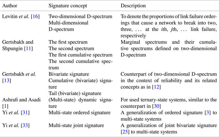
Table 1. Signature concepts for single binary-state coherent systems.

The above discussions are all for single binary-state coherent systems; for two (or more) binary-state coherent systems with shared i.i.d. components, concepts such as the joint signature were proposed; see Table 2 for details. Mohammadi [Reference Mohammadi18] considered m parallel systems and investigated the classification problem of their  $m!$ failure time permutations according to the
  $m!$ joint signatures. Furthermore, Mohammadi [Reference Mohammadi19] presented discussions for m coherent systems on related issues and the joint reliability signature of several
  $k$-out-of-
 $n$ systems was studied by Mohammadi [Reference Mohammadi20].
Table 2. Signature concepts for binary-state coherent systems with shared components.

The signature and its related concepts can be used effectively for stochastic comparisons of systems. For coherent systems with the same number of i.i.d. components, Kochar et al. [Reference Kochar, Mukerjee and Samaniego15] provided sufficient conditions for comparing the lifetimes according to the usual stochastic ordering, the hazard rate ordering, and the likelihood ratio ordering. Later, Navarro et al. [Reference Navarro, Ruiz and Sandoval22] considered coherent systems with the same number of exchangeable components and derived sufficient conditions for the comparison of their lifetimes based on the same three orders. Block et al. [Reference Block, Dugas, Samaniego, Balakrishnan, Castillo and Sarabia4] provided necessary and sufficient conditions for the three orders. For the comparison of coherent or mixed systems with different numbers of i.i.d. components (i.e., different sizes), Navarro et al. [Reference Navarro, Samaniego, Balakrishnan and Bhattacharya26] presented a transformation formula for their signatures by using the triangle rule of order statistics, and thence introduced the notion of equivalent systems. Lindqvist et al. [Reference Lindqvist, Samaniego and Huseby17] investigated the existence problem of equivalent systems of different sizes among coherent systems. For the comparison of used coherent systems with i.i.d. components, Navarro et al. [Reference Navarro, Balakrishnan and Samaniego21] presented sufficient conditions for the three orders. Burkschat and Navarro [Reference Burkschat and Navarro5] considered comparisons of systems with dependent components based on sequential order statistics.
The signature and its related concepts were first developed for binary-state systems. Later, due to the increasing importance of multi-state system modeling in practice, concepts of multi-state signatures got introduced into the literature; see Table 3 for details on multi-state coherent systems with binary-state components. Later, based on the bivariate signature in Gertsbakh et al. [Reference Gertsbakh, Shpungin and Spizzichino13], Da and Hu [Reference Da, Hu, Li and Li8] gave an equivalent definition of it from the view of probability as  ${\it{\boldsymbol{s}}}= ({s_{l,r}},1 \le l,r \le n)$ with
  ${s_{i,j}} = {{\mathbb P}}\{ {T_1} = {X_{i:n}},{T_2} = {X_{j:n}}\} \times {I_{\{ 1 \le i < j \le n\}}}$, where
  ${T_1}$ is the time that a ternary system enters state
  $1$ from state
  $2$ and
  ${T_2}$ is the later time that the same system enters state
  $0$. Ashrafi and Asadi [Reference Ashrafi and Asadi2] studied stochastic comparisons of ternary-state systems with same size or different sizes through their signature matrices. Zarezadeh et al. [Reference Zarezadeh, Asadi and Eftekhar37] discussed the joint probability density function and some information measures for system lifetimes of a multi-state system by using its signature. Recently, Yi et al. [Reference Yi, Balakrishnan and Cui32] examined some stochastic comparisons of multi-state systems of different sizes. Navarro and Spizzichino [Reference Navarro and Spizzichino27] studied stochastic comparisons of multi-state systems based on the signature and aggregation function by using decompositions of fuzzy measures.
Table 3. Signature concepts for multi-state coherent systems with binary-state components.
The above discussions were all for multi-state systems with binary-state components. For binary-state systems with multi-state components, Gertsbakh et al. [Reference Gertsbakh, Shpungin and Vaisman14] proposed the concept of ternary D-spectrum along the lines of D-spectrum for systems with binary-state components. Eryilmaz and Tuncel [Reference Eryilmaz and Tuncel10] generalized the survival signature to a certain class of multi-state systems with multi-state components that is in state j or above if j different rules get satisfied. Da Costa Bueno [Reference Da Costa Bueno9] introduced a multi-state monotone system signature for a multi-state system with multi-state components, with the lifetimes of components at different levels being all exchangeable. Yi et al. [Reference Yi, Cui and Balakrishnan36] provided a new computational method for survival signatures of multi-state consecutive-k systems with multi-state components. Yi et al. [Reference Yi, Balakrishnan and Li34] presented explicit formulas of multi-state (survival) signatures for a series/parallel/recurrent structure of given modules.
In the present work, we consider comparisons of joint signatures for binary-state and multi-state systems of different sizes along the lines of Navarro et al. [Reference Navarro, Samaniego, Balakrishnan and Bhattacharya26] and Yi et al. [Reference Yi, Balakrishnan and Cui32]. This work is of interest as one will often be interested in comparing an old structure with a new one when reconstruction is being considered in the design phase and that the two structures may then be of different sizes. To facilitate such comparisons through the use of signatures, transformation formulas between the signatures of different sizes are needed. Moreover, it is common to have systems with shared components in practice, but the comparisons of joint signatures with different sizes have not been discussed in the literature yet. Here, based on the joint signature of Navarro et al. [Reference Navarro, Samaniego and Balakrishnan25] for pairs of binary-state systems and the multi-state joint signature of Yi et al. [Reference Yi, Balakrishnan and Cui33] for pairs of multi-state systems, some transformation formulas are presented for pairs of binary-state and multi-state systems with different sizes. With these formulas, stochastic comparisons based on joint signatures become possible for any pair of systems. Results obtained here can be applied to many practical systems in reliability and network theory. For example, in the case of logistic network systems, one may be interested in the comparison of a current network structure and its past structure after the breakdown of some warehouse nodes.
This work discusses the comparison of joint signatures of different sizes. In Section 2, we first investigate the relationship between the joint signatures of two pairs of equivalent binary-state semi-coherent or mixed systems of different sizes by using a generalized triangle rule for the joint distribution of order statistics. Here, semi-coherent systems are systems whose reliabilities will not decrease with improvement of any component, which will simply be coherent systems if there is no irrelevant component in them. Also, mixed systems are stochastic mixtures of coherent systems of a given size. Next, in Section 3, we present similar discussions for multi-state systems of different sizes. The theoretical results established in Sections 2 and 3 are illustrated by means of some examples in Section 4. Finally, some conclusions and discussions are provided in Section 5.
2. Equivalency in joint signatures for binary-state systems of different sizes
In this section, we show how comparative results of joint signatures can be applied to binary-state systems of different sizes based on components with i.i.d. lifetimes. As done originally by Navarro et al. [Reference Navarro, Samaniego and Balakrishnan25], the joint signature can be defined for a pair of binary-state semi-coherent or mixed systems as follows.
Definition 2.1. Let  ${T_1}$ and
  ${T_2}$ be the lifetimes of two binary-state semi-coherent or mixed systems with m i.i.d. binary-state components, respectively. Let the lifetimes of the m components be denoted by
  ${X_1}, \ldots ,{X_m}$, and their common continuous distribution function be
  $F(x)\textrm{ }(x \ge 0)$. The matrix
  ${\it{\boldsymbol{s}}} = ({s_{i;j}},1 \le i,j \le m)$ is then called the joint signature of the two systems, where
  ${s_{i;j}} = {{\mathbb P}}\{ {T_1} = {X_{i:m}},{T_2} = {X_{j:m}}\}$, for
  $i,j = 1, \ldots ,m$, with
  ${X_{i:m}}$ and
  ${X_{j:m}}$ being the
  $ith$ and
  $jth$ order statistics among
  ${X_1}, \ldots ,{X_m}$.
Remark 2.1. The joint signature seems similar to the bivariate signature [Reference Da, Hu, Li and Li8] in formula, but they are two different concepts. The bivariate signature is for a single multi-state system and its elements  ${s_{i,j}} = 0$ for all
  $i < j$, while the joint signature is for two binary-state systems that share components and all its elements
  ${s_{i;j}}$ could be positive.
Before we consider the equivalency between two pairs of systems, the triangle rule for a single order statistic in Lemma 2.2 of Navarro et al. [Reference Navarro, Samaniego, Balakrishnan and Bhattacharya26] needs to be generalized as follows.
Lemma 2.1. Suppose the random variables  ${X_1}, \ldots ,{X_{m + 1}}$ are i.i.d. with a common continuous distribution function
  $F(x)\textrm{ }(x \ge 0)$. Then, for
  $1 \le k \le r \le m,$ the order statistic vector
  $({X_{k:m}},{X_{r:m}})$ has the same probability distribution as that of
 $$\left\{ {\begin{array}{*{20}{l}} {({X_{k + 1:m + 1}},{X_{r + 1:m + 1}})}& {with\textrm{ }probability\textrm{ }\dfrac{k}{{m + 1}},}\\ {({X_{k:m + 1}},{X_{r + 1:m + 1}})}& {with\textrm{ }probability\textrm{ }\dfrac{{r - k}}{{m + 1}},}\\ {({X_{k:m + 1}},{X_{r:m + 1}})}& {with\textrm{ }probability\textrm{ }\dfrac{{m + 1 - r}}{{m + 1}},} \end{array}} \right.$$
and for  $1 \le r < k \le m,$ the order statistic vector
  $({X_{k:m}},{X_{r:m}})$ has the same probability distribution as that of
 $$\left\{ {\begin{array}{*{20}{l}} {({X_{k + 1:m + 1}},{X_{r + 1:m + 1}})}& {with\;probability\;\dfrac{r}{{m + 1}},}\\ {({X_{k + 1:m + 1}},{X_{r:m + 1}})}& {with\;probability\;\dfrac{{k - r}}{{m + 1}},}\\ {({X_{k:m + 1}},{X_{r:m + 1}})}& {with\;probability\;\dfrac{{m + 1 - k}}{{m + 1}}.} \end{array}} \right.$$
Proof Choose a subset of size m from  $\{ {X_1}, \ldots ,{X_{m + 1}}\}$ randomly, and denote it by
  $\{ {Z_1}, \ldots ,{Z_m}\} .$ Then, in this process, each element in
  $\{ {X_1}, \ldots ,{X_{m + 1}}\}$ may be removed with probability
  $1/(m + 1)$ since
  ${X_1}, \ldots ,{X_{m + 1}}$ are i.i.d. random variables. Denote the
  $k\textrm{th}$ order statistic among
  $\{ {X_1}, \ldots ,{X_{m + 1}}\}$ as
  ${X_{k:m + 1}}$
  $(k = 1, \ldots ,m + 1)$ and the
  $k\textrm{th}$ order statistic among
  $\{ {Z_1}, \ldots ,{Z_m}\}$ as
  ${Z_{k:m}}$
  $(k = 1, \ldots ,m)$. Then, we have, for
  $1 \le k \le r \le m,$ the order statistic vector
  $({Z_{k:m}},{Z_{r:m}})$ will be distributed as
  $({X_{k + 1:m + 1}},{X_{r + 1:m + 1}})$ with probability
  $k/(m + 1)$ if the removed element is in the subset
  $\{ {X_{1:m + 1}}, \ldots ,{X_{k:m + 1}}\} ,$ will be distributed as
  $({X_{k:m + 1}},{X_{r + 1:m + 1}})$ with probability
  $(r - k)/(m + 1)$ if the removed element is in the subset
  $\{ {X_{k + 1:m + 1}}, \ldots ,{X_{r:m + 1}}\} ,$ and will be distributed as
  $({X_{k:m + 1}},{X_{r:m + 1}})$ with probability
  $(m + 1 - r)/(m + 1)$ if the removed element is in the subset
  $\{ {X_{r + 1:m + 1}}, \ldots ,{X_{m + 1:m + 1}}\} .$ Hence, the required result obtained.
As in Navarro et al. [Reference Navarro, Samaniego, Balakrishnan and Bhattacharya26], two pairs of binary-state systems are said to be equivalent if the joint distribution of system lifetimes  ${T_1},{T_2}$ in each pair is identical. Let
  ${\it{\boldsymbol{s}}} = ({s_{k;r}},1 \le k,r \le m)$ be the joint signature of two binary-state semi-coherent or mixed systems comprising m binary-state components with continuous i.i.d. lifetimes. Then, from Lemma 2.1, their equivalent system pair with
  $m + 1$ components has their joint signature vector as
 $${{\it{\boldsymbol{s}}} ^\ast } = \sum\limits_{1 \le k,r \le m} {{s_{k;r}}{\it{\boldsymbol{s}}} _{k;r:m}^\ast } ,$$
where for  $1 \le k \le r \le m$,
 $${\it{\boldsymbol{s}}} _{k;r:m}^\ast{=} \frac{k}{{m + 1}}{{\it{\boldsymbol{s}}} _{k + 1;r + 1:m + 1}} + \frac{{r - k}}{{m + 1}}{{\it{\boldsymbol{s}}} _{k;r + 1:m + 1}} + \frac{{m + 1 - r}}{{m + 1}}{{\it{\boldsymbol{s}}} _{k;r:m + 1}};$$
and for  $1 \le r < k \le m$,
 $${\it{\boldsymbol{s}}} _{k;r:m}^\ast{=} \frac{r}{{m + 1}}{{\it{\boldsymbol{s}}} _{k + 1;r + 1:m + 1}} + \frac{{k - r}}{{m + 1}}{{\it{\boldsymbol{s}}} _{k + 1,r:m + 1}} + \frac{{m + 1 - k}}{{m + 1}}{{\it{\boldsymbol{s}}} _{k,r:m + 1}}.$$
 Here,  ${\it{\boldsymbol{s}}} _{k;r:m}^\ast$ is the joint signature of the equivalent system with size
  $m + 1$ for a
  $k$-out-of-
 $m$:
$m$: $F$ system and an
  $r$-out-of-
 $m$:
$m$: $F$ system that share m i.i.d. binary-state components; also,
  ${{\it{\boldsymbol{s}}} _{k;r:m + 1}}$ is the joint signature of a
  $k$-out-of-
 $m + 1$:
 $F$ system and an
  $r$-out-of-
 $m + 1$:
 $F$ system that share
  $m + 1$ i.i.d. binary-state component, and specifically, there is only one positive element in
  ${{\it{\boldsymbol{s}}} _{k;r:m + 1}}.$ The pertinent discussion is similar to Theorem 2.2 in Yi et al. [Reference Yi, Balakrishnan and Cui32], and is, therefore, not presented here for conciseness. Then, the relationship of joint signatures can be established for two pairs of binary-state systems of different sizes as follows.
Theorem 2.1. Let  ${\it{\boldsymbol{s}}} = ({s_{k;r}},1 \le k,r \le m)$
  $(m \ge 2)$ be the joint signature of two binary-state semi-coherent or mixed systems based on the m components with continuous i.i.d. lifetimes. Then, an equivalent pair of systems with
  $m + 1$ components has their joint signature as
  ${{\it{\boldsymbol{s}}} ^\mathrm{\ast }} = (s_{i;j}^\mathrm{\ast },1 \le k,r \le m + 1)$, where
 $$s_{i;j}^\ast{=} \frac{{i \wedge j - 1}}{{m + 1}}{s_{i - 1;j - 1}} + \frac{{j - i - 1}}{{m + 1}}{s_{i;j - 1}}{I_{\{ i < j\} }} + \frac{{i - j - 1}}{{m + 1}}{s_{i - 1;j}}{I_{\{ j < i\} }} + \frac{{m + 1 - i \vee j}}{{m + 1}}{s_{i;j}}.$$
Proof From the discussions above and Theorem 2.3 in Yi et al. [Reference Yi, Balakrishnan and Cui32], we have
 $${{\it{\boldsymbol{s}}} ^\ast } = \sum\limits_{1 \le k \le r \le m} {{s_{k;r}}{\it{\boldsymbol{s}}} _{k;r:m}^\ast } \textrm{ + }\sum\limits_{1 \le r < k \le m} {{s_{k;r}}{\it{\boldsymbol{s}}} _{k;r:m}^\ast } ,$$
where the first term can be represented as
 $$\sum\limits_{1 \le k \le r \le m} {{s_{k;r}}{\it{\boldsymbol{s}}} _{k;r:m}^\ast } = \sum\limits_{1 \le i \le j \le m + 1} {\left( {\frac{{i - 1}}{{m + 1}}{s_{i - 1;j - 1}} + \frac{{j - i - 1}}{{m + 1}}{s_{i;j - 1}}{I_{\{ i < j\} }} + \frac{{m + 1 - j}}{{m + 1}}{s_{i;j}}} \right){{\it{\boldsymbol{s}}} _{i;j:m + 1}}} ,$$
and for the second term, we similarly have
 \begin{align*}\sum\limits_{1 \le r < k \le m} {{s_{k;r}}{\it{\boldsymbol{s}}} _{k;r:m}^\ast } & =\sum\limits_{1 \le r < k \le m} {{s_{k;r}}\left( {\dfrac{r}{{m + 1}}{{\it{\boldsymbol{s}}} _{k + 1;r + 1:m + 1}} + \dfrac{{k - r}}{{m + 1}}{{\it{\boldsymbol{s}}} _{k + 1;r:m + 1}} + \dfrac{{m + 1 - k}}{{m + 1}}{{\it{\boldsymbol{s}}} _{k;r:m + 1}}} \right)} \\ & =\sum\limits_{1 \le r < k \le m} {\dfrac{{r{s_{k;r}}}}{{m + 1}}{{\it{\boldsymbol{s}}} _{k + 1;r + 1:m + 1}}} + \sum\limits_{1 \le r < k \le m} {\dfrac{{(k - r){s_{k;r}}}}{{m + 1}}{{\it{\boldsymbol{s}}} _{k + 1;r:m + 1}}}\\ &\quad + \sum\limits_{1 \le r < k \le m} {\dfrac{{(m + 1 - k){s_{k;r}}}}{{m + 1}}{{\it{\boldsymbol{s}}} _{k;r:m + 1}}} \\ & =\sum\limits_{2 \le j < i \le m + 1} {\dfrac{{(j - 1){s_{i - 1;j - 1}}}}{{m + 1}}{{\it{\boldsymbol{s}}} _{i;j:m + 1}}} + \sum\limits_{1 \le j < i - 1 \le m} {\dfrac{{(i - j - 1){s_{i - 1;j}}}}{{m + 1}}{{\it{\boldsymbol{s}}} _{i;j:m + 1}}}\\ &\quad + \sum\limits_{1 \le j < i \le m} {\dfrac{{(m + 1 - i){s_{i;j}}}}{{m + 1}}{{\it{\boldsymbol{s}}} _{i;j:m + 1}}} \\ & =\sum\limits_{1 \le j < i \le m + 1} {\left( {\dfrac{{j - 1}}{{m + 1}}{s_{i - 1;j - 1}} + \dfrac{{i - j - 1}}{{m + 1}}{s_{i - 1;j}} + \dfrac{{m + 1 - i}}{{m + 1}}{s_{i;j}}} \right){{\it{\boldsymbol{s}}} _{i;j:m + 1}}} . \end{align*}
Upon combining the above two expressions, we obtain
 \begin{align*}{{\it{\boldsymbol{s}}} ^\ast }&= \sum\limits_{1 \le i,j \le m + 1} \left( {\frac{{i \wedge j - 1}}{{m + 1}}{s_{i - 1;j - 1}} + \frac{{j - i - 1}}{{m + 1}}{s_{i;j - 1}}{I_{\{ i < j\} }} + \frac{{i - j - 1}}{{m + 1}}{s_{i - 1;j}}{I_{\{ j < i\} }} + \frac{{m + 1 - i \vee j}}{{m + 1}}{s_{i;j}}} \right)\notag\\ &\quad {{\it{\boldsymbol{s}}} _{i;j:m + 1}} ,\end{align*}
which completes the proof of the theorem.
Remark 2.2. Throughout this work, we use  $i \vee j$ and
  $i \wedge j$ to denote the larger one and the smaller one among numbers i and j. Besides, terms like
  ${s_{i,j}}$ with
  $i = 0$ or
  $j = 0$ are interpreted as the probabilities for cases that one of the two system fails with no component failure, which is impossible under our assumption, so that
  ${s_{i,j}} = 0$ for
  $i = 0$ or
  $j = 0$. Note that these terms always appear with zero coefficient, which means actually they are not included in the formula of
  ${\textbf{s}^\ast }$.
In Theorem 2.1, the relationship between joint signatures is established for a pair of binary-state systems with m shared components and their equivalent pair of binary-state systems with  $m + 1$ shared components. To obtain a more general result, a general version of Lemma 2.1 is proved in the following lemma.
Lemma 2.2. Suppose the random variables  ${X_1}, \ldots ,{X_{m + l}}$ are i.i.d. with a common continuous distribution function
  $F(x)\textrm{ }(x \ge 0)$. Then, for
  $1 \le k \le r \le m < m + l$, the order statistic vector
  $({X_{k:m}},{X_{r:m}})$ has the same probability distribution as
  $({X_{i:m + l}},{X_{j:m + l}})$ with probability
 $${\left( {\begin{array}{*{20}{c}} {m + l}\\ m \end{array}} \right)^{ - 1}}\left( {\begin{array}{*{20}{c}} {i - 1}\\ {k - 1} \end{array}} \right){\left( {\begin{array}{*{20}{c}} {j - i - 1}\\ {r - k - 1} \end{array}} \right)^{{I_{\{ j > i\} }}}}\left( {\begin{array}{*{20}{c}} {m + l - j}\\ {m - r} \end{array}} \right),$$
where  $(i,j) \in {\Omega _{m,l}}(k;r) =$
  $\{ (k + a,r + b):a = 0, \ldots ,l\textrm{ and }b = a, \ldots ,l + (a - l){I_{\{ k = r\} }}\};$ and for
  $1 \le r < k \le m < m + l,$ the order statistic vector
  $({X_{k:m}},{X_{r:m}})$ has the same probability distribution as
  $({X_{i:m + l}},{X_{j:m + l}})$ with probability
 $${\left( {\begin{array}{*{20}{c}} {m + l}\\ m \end{array}} \right)^{ - 1}}\left( {\begin{array}{*{20}{c}} {j - 1}\\ {r - 1} \end{array}} \right)\left( {\begin{array}{*{20}{c}} {i - j - 1}\\ {k - r - 1} \end{array}} \right)\left( {\begin{array}{*{20}{c}} {m + l - i}\\ {m - k} \end{array}} \right),$$
where  $(i,j) \in {\Omega _{m,l}}(k;r) = \{ (k + a,r + b):a = 0, \ldots ,l\textrm{ and }b = 0, \ldots ,a\}\textrm{.}$
Proof As in Lemma 2.1, choose a subset of size m from  $\{ {X_1}, \ldots ,{X_{m + l}}\}$ randomly, and denote it by
  $\{ {Z_1}, \ldots ,{Z_m}\} .$ Then, in this process, l elements in
  $\{ {X_1}, \ldots ,{X_{m + l}}\}$ will be removed with an equal probability since
  ${X_1}, \ldots ,{X_{m + l}}$ are i.i.d. random variables. For
  $1 \le k \le r \le m,$ the order statistic vector
  $({X_{i:m + l}},{X_{j:m + l}})$ will be distributed as
  $({Z_{k:m}},{Z_{r:m}})$ with probability
 $${\left( {\begin{array}{*{20}{c}} {m + l}\\ m \end{array}} \right)^{ - 1}}\left( {\begin{array}{*{20}{c}} {i - 1}\\ {k - 1} \end{array}} \right){\left( {\begin{array}{*{20}{c}} {j - i - 1}\\ {r - k - 1} \end{array}} \right)^{{I_{\{ j > i\} }}}}\left( {\begin{array}{*{20}{c}} {m + l - j}\\ {m - r} \end{array}} \right)$$
if there are  $k - 1$ elements chosen from the subset
  $\{ {X_{1:m + l}}, \ldots ,{X_{i - 1:m + l}}\} ,$
  $r - k - 1$ elements chosen from the subset
  $\{ {X_{i + 1:m + l}}, \ldots ,{X_{j - 1:m + l}}\} , \ldots ,$
  $m - r$ elements chosen from the subset
  $\{ {X_{j + 1:m + l}}, \ldots ,{X_{m + l:m + l}}\}$, and elements
  ${X_{i:m + l}},{X_{j:m + l}}$ are chosen for sure. Here, we also have
  $(i,j) = (k + a,r + b)$ with
  $a = 0, \ldots ,l$ and
  $b = a, \ldots ,l + (a - l){I_{\{ k = r\} }}$. Thus, the required result follows.
The following theorem can then be proved directly from Lemma 2.2 for the relationship between joint signatures of a pair of binary-state systems with m shared components and their equivalent pair of binary-state systems with  $m + l$ shared components.
Theorem 2.2. Let  ${\it{\boldsymbol{s}}} = ({s_{k;r}},1 \le k,r \le m)$ be the joint signature of two binary-state semi-coherent or mixed systems comprising m binary-state components with i.i.d. lifetimes. Then, an equivalent pair of systems with
  $m + l$ components has their joint signature as
 $${{\it{\boldsymbol{s}}} ^{(l)\ast }} = \sum\limits_{1 \le k,r \le m} {{s_{k;r}}{\it{\boldsymbol{s}}} _{k;r:m}^{(l)\ast }} ,$$
where
 $${\Omega _{m,l}}(k;r) = \{ (k + a,r + b):a = 0, \ldots ,l\textrm{ }and\textrm{ }b = a{I_{\{ k \le r\} }}, \ldots ,l + (a - l){I_{\{ k \ge r\} }}\} ,$$
and
 $${\it{\boldsymbol{s}}}_{k;r:m}^{(l)\ast } = \sum\limits_{(i;j) \in {\Omega _{m,l}}(k;r)} {{{\left( {\begin{array}{*{20}{c}} {m + l}\\ m \end{array}} \right)}^{ - 1}}\left( {\begin{array}{*{20}{c}} {i \wedge j - 1}\\ {k \wedge r - 1} \end{array}} \right){{\left( {\begin{array}{*{20}{c}} {|{j - i} |- 1}\\ {|{r - k} |- 1} \end{array}} \right)}^{{I_{\{ j \ne i\} }}}}\left( {\begin{array}{*{20}{c}} {m + l - i \vee j}\\ {m - k \vee r} \end{array}} \right) \cdot {{\it{\boldsymbol{s}}} _{i;j:m + l}}}$$
is the joint signature of an equivalent pair of systems with  $m + l$ shared components for a
  $k$-out-of-
  $m$:
$m$:  $F$ system and an
  $r$-out-of-
  $m$:
$m$:  $F$ system with m shared components.
Remark 2.3. Based on the discussions above, by exchanging the order of summation, we get
 $${{\it{\boldsymbol{s}}} ^{(l)\ast }} = \sum\limits_{1 \le i,j \le m + l} {{{\it{\boldsymbol{s}}} _{i;j:m + l}}\sum\limits_{(k;r) \in \Omega _{m,l}^{ - 1}(i;j)} {{{\left( {\begin{array}{*{20}{c}} {m + l}\\ m \end{array}} \right)}^{ - 1}}\left( {\begin{array}{*{20}{c}} {i \wedge j - 1}\\ {k \wedge r - 1} \end{array}} \right){{\left( {\begin{array}{*{20}{c}} {|{j - i} |- 1}\\ {|{r - k} |- 1} \end{array}} \right)}^{{I_{\{ j \ne i\} }}}}\left( {\begin{array}{*{20}{c}} {m + l - i \vee j}\\ {m - k \vee r} \end{array}} \right){s_{k;r}}} } ,$$
where
 $$\Omega _{m,l}^{ - 1}(i;j) = \{ (i - a,j - b):a = 0, \ldots ,i \wedge l\textrm{ and }b = a{I_{\{ i \le j\} }}, \ldots ,j \wedge (l + (a - l){I_{\{ i \ge j\} }})\} .$$
 Then, we have  ${{\it{\boldsymbol{s}}} ^{(l)\ast }} = (s_{i;j}^{(l)\ast },1 \le i,j \le m + l)$, where
 $$s_{i;j}^{(l)\ast } = \sum\limits_{(k;r) \in \Omega _{m,l}^{ - 1}(i;j)} {{{\left( {\begin{array}{*{20}{c}} {m + l}\\ m \end{array}} \right)}^{ - 1}}\left( {\begin{array}{*{20}{c}} {i \wedge j - 1}\\ {k \wedge r - 1} \end{array}} \right){{\left( {\begin{array}{*{20}{c}} {|{j - i} |- 1}\\ {|{r - k} |- 1} \end{array}} \right)}^{{I_{\{ j \ne i\} }}}}\left( {\begin{array}{*{20}{c}} {m + l - i \vee j}\\ {m - k \vee r} \end{array}} \right){s_{k;r}}} .$$
 Specifically, for  $l = 1$, we have
 \begin{align*}\Omega _{m,1}^{ - 1}(i;j) =& \{ (i - a,j - b):a = 0,1\textrm{ and }b = a{I_{\{ i \le j\} }}, \ldots ,1 + (a - 1){I_{\{ i \ge j\} }}\} \\ =& {I_{\{ i < j\} }}\{ (i,j),(i,j - 1),(i - 1,j - 1)\} + {I_{\{ i = j\} }}\{ (i,j),(i - 1,j - 1)\} \\& + {I_{\{ i > j\} }}\{ (i,j),(i - 1,j),(i - 1,j - 1)\} \end{align*}
and
 \begin{align*} s_{i;j}^{(1)\ast } & =\sum\limits_{(k;r) \in \Omega _{m,1}^{ - 1}(i;j)} {\dfrac{1}{{m + 1}}\left( {\begin{array}{*{20}{c}} {i \wedge j - 1}\\ {k \wedge r - 1} \end{array}} \right){{\left( {\begin{array}{*{20}{c}} {|{j - i} |- 1}\\ {|{r - k} |- 1} \end{array}} \right)}^{{I_{\{ j \ne i\} }}}}\left( {\begin{array}{*{20}{c}} {m + 1 - i \vee j}\\ {m - k \vee r} \end{array}} \right){s_{k;r}}} \\ & =\frac{1}{{m + 1}}\left( {\begin{array}{*{20}{c}} {m + 1 - i \vee j}\\ {m - i \vee j} \end{array}} \right){s_{i;j}} + \frac{1}{{m + 1}}\left( {\begin{array}{*{20}{c}} {j - i - 1}\\ {j - i - 2} \end{array}} \right){s_{i;j - 1}}{I_{\{ i < j\} }}\\& \quad + \frac{1}{{m + 1}}\left( {\begin{array}{*{20}{c}} {i - j - 1}\\ {i - j - 2} \end{array}} \right){s_{i - 1;j}}{I_{\{ i > j\} }} + \frac{1}{{m + 1}}\left( {\begin{array}{*{20}{c}} {i \wedge j - 1}\\ {i \wedge j - 2} \end{array}} \right){s_{i - 1;j - 1}}\\& = \frac{{m + 1 - i \vee j}}{{m + 1}}{s_{i;j}}\textrm{ + }\frac{{j - i - 1}}{{m + 1}}{s_{i;j - 1}}{I_{\{ i < j\} }} + \frac{{i - j - 1}}{{m + 1}}{s_{i - 1;j}}{I_{\{ i > j\} }} + \frac{{i \wedge j - 1}}{{m + 1}}{s_{i - 1;j - 1}}, \end{align*}
which is exactly the result in Theorem 2.1.
3. Equivalency in joint signatures for multi-state systems of different sizes
In this section, the results established in the last section are generalized to multi-state systems of different sizes based on the components with i.i.d. lifetimes. As shown in Yi et al. [Reference Yi, Balakrishnan and Cui33], the (multi-state) joint signature can be defined for a pair of multi-state semi-coherent or mixed systems as follows.
Definition 3.1. Let  $T_k^{(1)}$ and
  $T_k^{(2)}$
  $(k = 1, \ldots ,n)$ be the first times that two multi-state semi-coherent or mixed systems, with state space
  $\tilde{S} = \{ 0, \ldots ,n\}$ and m i.i.d. binary-state components, enter state
  $n - k$ or below, respectively. Denote the lifetimes of the m components by
  ${X_1}, \ldots ,{X_m}$, and their common continuous distribution function by
  $F(x)\textrm{ }(x \ge 0)$. Then, the matrix
  ${\it{\boldsymbol{s}}} = ({s_{{i_1}, \ldots ,{i_n};{j_1}, \ldots ,{j_n}}},1 \le {i_1}, \ldots ,{i_n},{j_1}, \ldots ,{j_n} \le m)$ is called the multi-state joint signature of the two systems associated with
  $(T_1^{(1)}, \ldots ,T_n^{(1)},T_1^{(2)}, \ldots ,T_n^{(2)})$, where
  ${s_{{i_1}, \ldots ,{i_n};{j_1}, \ldots ,{j_n}}} = {{\mathbb P}}\{ T_k^{(1)} = {X_{{i_k}:m}},T_k^{(2)} = {X_{{j_k}:m}},k = 1, \ldots ,n\} ,$ for
  ${i_1}, \ldots ,{i_n},{j_1}, \ldots ,{j_n} \in {\{ }1, \ldots ,m\}$, with
  ${X_{{i_k}:m}}$ and
  ${X_{{j_k}:m}}$ being the
  ${i_k}th$ and
  ${j_k}th$ order statistics among
  ${X_1}, \ldots ,{X_m}$.
For comparison results based on joint signatures, a lemma similar to Lemmas 2.1 and 2.2 is as follows.
Lemma 3.1. Suppose the random variables  ${X_1}, \ldots ,{X_{m + 1}}$ are i.i.d. with a common continuous distribution function
  $F(x)\textrm{ }(x \ge 0)$. Then, for
  $1 \le {k_1} \le \cdots \le {k_n} \le m$ and
  $1 \le {r_1} \le \cdots \le {r_n} \le m,$ the order statistic vector
  $({X_{{k_1}:m}}, \ldots ,{X_{{k_n}:m}},{X_{{r_1}:m}}, \ldots ,{X_{{r_n}:m}})$ has the same probability distribution as
 $$\left\{ \begin{array}{l} ({X_{{k_1} + 1:m + 1}}, \ldots ,{X_{{k_n} + 1:m + 1}},{X_{{r_1} + 1:m + 1}}, \ldots ,{X_{{r_n} + 1:m + 1}})\ with\textrm{ }probability\textrm{ }\dfrac{{{k_1} \wedge {r_1}}}{{m + 1}}\\ ({X_{{k_1}:m + 1}}, \ldots ,{X_{{k_n}:m + 1}},{X_{{r_1}:m + 1}}, \ldots ,{X_{{r_n}:m + 1}})\ with\textrm{ }probability\textrm{ }\dfrac{{m + 1 - {k_n} \vee {r_n}}}{{m + 1}}\\ ({X_{{k_1}:m + 1}}, \ldots ,{X_{{k_j}:m + 1}},{X_{{k_{j + 1}} + 1:m + 1}}, \ldots ,{X_{{k_n} + 1:m + 1}},{X_{{r_1}:m + 1}}, \ldots ,{X_{{r_i}:m + 1}},{X_{{r_{i + 1}} + 1:m + 1}}, \ldots ,{X_{{r_n} + 1:m + 1}})\\ \quad \quad with\textrm{ }probability\textrm{ }\dfrac{{{r_{i + 1}} - {r_i}}}{{m + 1}}\textrm{ }for\textrm{ }j = 0, \ldots ,n,\textrm{ }i = {w_j} + 1, \ldots ,{w_{j + 1}} - 1\textrm{ }and\textrm{ }{w_j} + 1 < {w_{j + 1}}\\ ({X_{{k_1}:m + 1}}, \ldots ,{X_{{k_{j - 1}}:m + 1}},{X_{{k_j} + 1:m + 1}}, \ldots ,{X_{{k_n} + 1:m + 1}},{X_{{r_1}:m + 1}}, \ldots ,{X_{{r_{{w_j}}}:m + 1}},{X_{{r_{{w_j} + 1}} + 1:m + 1}}, \ldots ,{X_{{r_n} + 1:m + 1}})\\ \quad \quad with\textrm{ }probability\textrm{ }\dfrac{{{k_j} - {r_{{w_j}}}}}{{m + 1}}\textrm{ }for\textrm{ }j = 1, \ldots ,n\textrm{ }and\textrm{ }{w_{j - 1}} < {w_j}\\ ({X_{{k_1}:m + 1}}, \ldots ,{X_{{k_j}:m + 1}},{X_{{k_{j + 1}} + 1:m + 1}}, \ldots ,{X_{{k_n} + 1:m + 1}},{X_{{r_1}:m + 1}}, \ldots ,{X_{{r_{{w_j}}}:m + 1}},{X_{{r_{{w_j} + 1}} + 1:m + 1}}, \ldots ,{X_{{r_n} + 1:m + 1}})\\ \quad \quad with\textrm{ }probability\textrm{ }\dfrac{{{r_{{w_j} + 1}} - {k_j}}}{{m + 1}}\textrm{ }for\textrm{ }j = 1, \ldots ,n\textrm{ }and\textrm{ }{w_j} < {w_{j + 1}}\\ ({X_{{k_1}:m + 1}}, \ldots ,{X_{{k_j}:m + 1}},{X_{{k_{j + 1}} + 1:m + 1}}, \ldots ,{X_{{k_n} + 1:m + 1}},{X_{{r_1}:m + 1}}, \ldots ,{X_{{r_{{w_j}}}:m + 1}},{X_{{r_{{w_j} + 1}} + 1:m + 1}}, \ldots ,{X_{{r_n} + 1:m + 1}})\\ \quad \quad with\textrm{ }probability\textrm{ }\dfrac{{{k_{j + 1}} - {k_j}}}{{m + 1}}\textrm{ }for\textrm{ }j = 1, \ldots ,n - 1\textrm{ }and\textrm{ }{w_j} = {w_{j + 1}} \end{array} \right.,$$
where  ${k_{n + 1}} = m,\;{r_0} = {k_0} = 0$ and
  ${w_j},j = 0, \ldots ,n + 1$, is the largest one in
  $\{ i:{r_i} \le {k_j},i = 0, \ldots ,n\}$, and these notations will also be used in all the subsequent discussions.
Proof For  $1 \le {k_1} \le \cdots \le {k_n} \le m$ and
  $1 \le {r_1} \le \cdots \le {r_n} \le m$, let us denote
  ${k_{n + 1}} = m,{r_0} = {k_0} = 0$, and the largest one in
  $\{ i:{r_i} \le {k_j},i = 0, \ldots ,n\}$ by
  ${w_j},j = 0, \ldots ,n + 1$; see Figure 1 for a possible ordering of
  ${k_1}, \ldots ,{k_n},{r_1}, \ldots ,{r_n}$. Choose a subset of size m from
  $\{ {X_1}, \ldots ,{X_{m + 1}}\}$ randomly, and denote it by
  $\{ {Z_1}, \ldots ,{Z_m}\}$. Then, there are six cases to consider for the order statistic vector
  $({X_{{k_1}:m}}, \ldots ,{X_{{k_n}:m}},{X_{{r_1}:m}}, \ldots ,{X_{{r_n}:m}})$, as listed below:

Figure 1. A possible ordering of  ${k_1},{k_2}, \ldots ,{k_n},{r_1},{r_2}, \ldots ,{r_n}$ in Lemma 3.1.
Case 1: If the removed element is in the subset  $\{ {X_{1:m + 1}}, \ldots ,{X_{{k_1} \wedge {r_1}:m + 1}}\}$, the order statistic vector
  $({X_{{k_1}:m}}, \ldots ,{X_{{k_n}:m}},{X_{{r_1}:m}}, \ldots ,{X_{{r_n}:m}})$ will be distributed as
  $({X_{{k_1} + 1:m + 1}}, \ldots ,{X_{{k_n} + 1:m + 1}},{X_{{r_1} + 1:m + 1}}, \ldots ,{X_{{r_n} + 1:m + 1}})$ with probability
  $({k_1} \wedge {r_1})/(m + 1)$;
Case 2: If the removed element is in the subset  $\{ {X_{{k_n} \vee {r_n} + 1:m + 1}}, \ldots ,{X_{m + 1:m + 1}}\}$, the order statistic vector
  $({X_{{k_1}:m}}, \ldots ,{X_{{k_n}:m}},{X_{{r_1}:m}}, \ldots ,{X_{{r_n}:m}})$ will be distributed as
  $({X_{{k_1}:m + 1}}, \ldots ,{X_{{k_n}:m + 1}},{X_{{r_1}:m + 1}}, \ldots ,{X_{{r_n}:m + 1}})$ with probability
  $(m + 1 - {k_n} \vee {r_n})/(m + 1)$;
Case 3: If the removed element is in the subset  $\{ {X_{{r_i} + 1:m + 1}}, \ldots ,{X_{{r_{i + 1}}:m + 1}}\}$, where
  $i = {w_j} + 1, \ldots ,{w_{j + 1}} - 1,j = 0, \ldots ,n$ and
  ${w_j} + 1 < {w_{j + 1}}$ (there are at least two elements in
  ${r_i},\textrm{ }i = 1, \ldots ,n$, that satisfy
  ${k_j} < {r_i} \le {k_{j + 1}}$), the order statistic vector
  $({X_{{k_1}:m}}, \ldots ,{X_{{k_n}:m}},{X_{{r_1}:m}}, \ldots ,{X_{{r_n}:m}})$ will be distributed as
  $({X_{{k_1}:m + 1}}, \ldots ,{X_{{k_j}:m + 1}},{X_{{k_{j + 1}} + 1:m + 1}}, \ldots ,{X_{{k_n} + 1:m + 1}},{X_{{r_1}:m + 1}}, \ldots ,{X_{{r_i}:m + 1}},{X_{{r_{i + 1}} + 1:m + 1}}, \ldots ,{X_{{r_n} + 1:m + 1}})$ with probability
  $({r_{i + 1}} - {r_i})/(m + 1)$;
Case 4: If the removed element is in the subset  $\{ {X_{{r_{{w_j}}} + 1:m + 1}}, \ldots ,{X_{{k_j}:m + 1}}\}$, where
  ${w_{j - 1}} < {w_j},j = 1, \ldots ,n$ (there is at least one element in
  ${r_i},\textrm{ }i = 1, \ldots ,n$, that satisfy
  ${k_{j - 1}} < {r_i} \le {k_j}$), the order statistic vector
  $({X_{{k_1}:m}}, \ldots ,{X_{{k_n}:m}},{X_{{r_1}:m}}, \ldots ,{X_{{r_n}:m}})$ will be distributed as
  $({X_{{k_1}:m + 1}}, \ldots ,{X_{{k_{j - 1}}:m + 1}},{X_{{k_j} + 1:m + 1}}, \ldots ,{X_{{k_n} + 1:m + 1}},{X_{{r_1}:m + 1}}, \ldots ,{X_{{r_{{w_j}}}:m + 1}},{X_{{r_{{w_j} + 1}} + 1:m + 1}}, \ldots ,{X_{{r_n} + 1:m + 1}})$ with probability
  $({k_j} - {r_{{w_j}}})/(m + 1)$;
Case 5: If the removed element is in the subset  $\{ {X_{{k_j} + 1:m + 1}}, \ldots ,{X_{{r_{{w_j} + 1}}:m + 1}}\}$, where
  ${w_j} < {w_{j + 1}},j = 1, \ldots ,n$ (there is at least one element in
  ${r_i},\textrm{ }i = 1, \ldots ,n$, that satisfy
  ${k_j} < {r_i} \le {k_{j + 1}}$), the order statistic vector
  $({X_{{k_1}:m}}, \ldots ,{X_{{k_n}:m}},{X_{{r_1}:m}}, \ldots ,{X_{{r_n}:m}})$ will be distributed as
  $({X_{{k_1}:m + 1}}, \ldots ,{X_{{k_j}:m + 1}},{X_{{k_{j + 1}} + 1:m + 1}}, \ldots ,{X_{{k_n} + 1:m + 1}},{X_{{r_1}:m + 1}}, \ldots ,{X_{{r_{{w_j}}}:m + 1}},{X_{{r_{{w_j} + 1}} + 1:m + 1}}, \ldots ,{X_{{r_n} + 1:m + 1}})$ with probability
  $({r_{{w_j} + 1}} - {k_j})/(m + 1)$;
Case 6: Finally, if the removed element is in the subset  $\{ {X_{{k_j} + 1:m + 1}}, \ldots ,{X_{{k_{j + 1}}:m + 1}}\}$, where
  ${w_j} = {w_{j + 1}},j = 1, \ldots ,n - 1$ (there is no element in
  ${r_i},\textrm{ }i = 1, \ldots ,n$, that satisfies
  ${k_j} < {r_i} \le {k_{j + 1}}$), the order statistic vector
  $({X_{{k_1}:m}}, \ldots ,{X_{{k_n}:m}},{X_{{r_1}:m}}, \ldots ,{X_{{r_n}:m}})$ will be distributed as
  $({X_{{k_1}:m + 1}}, \ldots ,{X_{{k_j}:m + 1}},{X_{{k_{j + 1}} + 1:m + 1}}, \ldots ,{X_{{k_n} + 1:m + 1}},{X_{{r_1}:m + 1}}, \ldots ,{X_{{r_{{w_j}}}:m + 1}},{X_{{r_{{w_j} + 1}} + 1:m + 1}}, \ldots ,{X_{{r_n} + 1:m + 1}})$ with probability
  $({k_{j + 1}} - {k_j})/(m + 1)$.
The proof gets completed readily upon combining all the above facts.
As in Navarro et al. [Reference Navarro, Samaniego, Balakrishnan and Bhattacharya26], two pairs of multi-state systems are said to be equivalent if the joint distribution of system lifetimes  $T_1^{(1)}, \ldots ,T_n^{(1)},T_1^{(2)}, \ldots ,T_n^{(2)}$ in each pair are identical. Let
  ${\it{\boldsymbol{s}}} = ({s_{{k_1}, \ldots ,{k_n};{r_1}, \ldots ,{r_n}}},1 \le {k_1}, \ldots ,{k_n},{r_1}, \ldots ,{r_n} \le m)$
  $(m \ge 2)$ be the joint signature of two multi-state semi-coherent or mixed systems comprising m binary-state components with i.i.d. lifetimes. Then, from Lemma 3.1, an equivalent pair of systems with
  $m + 1$ components has the joint signature as
 $${{\it{\boldsymbol{s}}} ^\ast } = \sum\limits_{1 \le {k_1}, \ldots ,{k_n},{r_1}, \ldots ,{r_n} \le m} {{s_{{k_1}, \ldots ,{k_n};{r_1}, \ldots ,{r_n}}}{\it{\boldsymbol{s}}} _{{k_1}, \ldots ,{k_n};{r_1}, \ldots ,{r_n}:m}^\ast } ,$$
where  ${s_{{k_1}, \ldots ,{k_n};{r_1}, \ldots ,{r_n}}} \ne 0$ only for
  $1 \le {k_1} \le \cdots \le {k_n} \le m,1 \le {r_1} \le \cdots \le {r_n} \le m$, and
 \begin{align*} {\it{\boldsymbol{s}}} _{{k_1}, \ldots ,{k_n};{r_1}, \ldots ,{r_n}:m}^\ast = & \dfrac{{{k_1} \wedge {r_1}}}{{m + 1}}{{\it{\boldsymbol{s}}} _{{k_1} + 1, \ldots ,{k_n} + 1;{r_1} + 1, \ldots ,{r_n} + 1:m + 1}} + \dfrac{{m + 1 - {k_n} \vee {r_n}}}{{m + 1}}{{\it{\boldsymbol{s}}} _{{k_1}, \ldots ,{k_n};{r_1}, \ldots ,{r_n}:m + 1}}\\& {\kern 1pt} \textrm{ + }\sum\limits_{j = 0}^n {\sum\limits_{i = {w_j} + 1}^{{w_{j + 1}} - 1} {\dfrac{{{r_{i + 1}} - {r_i}}}{{m + 1}}{{\it{\boldsymbol{s}}} _{{k_1}, \ldots ,{k_j},{k_{j + 1}} + 1, \ldots ,{k_n} + 1;{r_1}, \ldots ,{r_i},{r_{i + 1}} + 1, \ldots ,{r_n} + 1:m + 1}}{I_{\{ {w_j} + 1 < {w_{j + 1}}\} }}} } \\& \textrm{ + }\sum\limits_{j = 1}^n {\dfrac{{{k_j} - {r_{{w_j}}}}}{{m + 1}}{{\it{\boldsymbol{s}}} _{{k_1}, \ldots ,{k_{j - 1}},{k_j} + 1, \ldots ,{k_n} + 1;{r_1}, \ldots ,{r_{{w_j}}},{r_{{w_j} + 1}} + 1, \ldots ,{r_n} + 1:m + 1}}{I_{\{ {w_{j - 1}} < {w_j}\} }}} \\& \textrm{ + }\sum\limits_{j = 1}^n {\dfrac{{{r_{{w_j} + 1}} - {k_j}}}{{m + 1}}{{\it{\boldsymbol{s}}} _{{k_1}, \ldots ,{k_j},{k_{j + 1}} + 1, \ldots ,{k_n} + 1;{r_1}, \ldots ,{r_{{w_j}}},{r_{{w_j} + 1}} + 1, \ldots ,{r_n} + 1:m + 1}}{I_{\{ {w_j} < {w_{j + 1}}\} }}} \\& \textrm{ + }\sum\limits_{j = 1}^{n - 1} {\dfrac{{{k_{j + 1}} - {k_j}}}{{m + 1}}{{\it{\boldsymbol{s}}} _{{k_1}, \ldots ,{k_j},{k_{j + 1}} + 1, \ldots ,{k_n} + 1;{r_1}, \ldots ,{r_{{w_j}}},{r_{{w_j} + 1}} + 1, \ldots ,{r_n} + 1:m + 1}}} {I_{\{ {w_j} = {w_{j + 1}}\} }}. \end{align*}
 Here,  ${\it{\boldsymbol{s}}} _{{k_1}, \ldots ,{k_n};{r_1}, \ldots ,{r_n}:m}^\ast$ is the joint signature of the pair of equivalent systems with size
  $m + 1$ for a
  $({k_n}, \ldots ,{k_1})$-out-of-
 $m$:
$m$: $F$ system and an
  $({r_n}, \ldots ,{r_1})$-out-of-
 $m$:
$m$: $F$ system with m shared components; also
  ${{\it{\boldsymbol{s}}} _{{k_1}, \ldots ,{k_n};{r_1}, \ldots ,{r_n}:m + 1}}$ is the joint signature of a
  $({k_n}, \ldots ,{k_1})$-out-of-
 $m + 1$:
 $F$ system and an
  $({r_n}, \ldots ,{r_1})$-out-of-
 $m + 1$:
 $F$ system with
  $m + 1$ shared components, and specifically, there is only one positive element in
  ${{\it{\boldsymbol{s}}} _{{k_1}, \ldots ,{k_n};{r_1}, \ldots ,{r_n}:m + 1}}$. Then, analogous to Theorem 2.1, the relationship of joint signatures of two pairs of multi-state systems of different sizes can be established as in the following theorem.
Theorem 3.1. Let  ${\it{\boldsymbol{s}}} = ({s_{{k_1}, \ldots ,{k_n};{r_1}, \ldots ,{r_n}}},1 \le {k_1}, \ldots ,{k_n},{r_1}, \ldots ,{r_n} \le m)$
  $(m \ge 2)$ be the joint signature of two multi-state semi-coherent or mixed systems based on the m binary-state components with continuous i.i.d. lifetimes. Then, an equivalent pair of systems with
  $m + 1$ binary-state components has their joint signature as
 $${{\it{\boldsymbol{s}}} ^\mathrm{\ast }} = (s_{{i_1}, \ldots ,{i_n};{j_1}, \ldots ,{j_n}}^\mathrm{\ast },\;1 \le {i_1}, \ldots ,{i_n},{j_1}, \ldots ,{j_n} \le m + 1),$$
where
 \begin{align*} s_{{i_1}, \ldots ,{i_n};{j_1}, \ldots ,{j_n}}^\ast{=} & \dfrac{{{i_1} \wedge {j_1} - 1}}{{m + 1}}{s_{{i_1} - 1, \ldots ,{i_n} - 1;{j_1} - 1, \ldots ,{j_n} - 1}}\textrm{ + }\dfrac{{m + 1 - {i_n} \vee {j_n}}}{{m + 1}}{s_{{i_1}, \ldots ,{i_n};{j_1}, \ldots ,{j_n}}}\\ & \textrm{ + }\sum\limits_{b = 0}^n {\sum\limits_{a = {w_b} + 1}^{{w_{b + 1}} - 1} {\dfrac{{{j_{a + 1}} - {j_a} - 1}}{{m + 1}}{s_{{i_1}, \ldots ,{i_b},{i_{b + 1}} - 1, \ldots ,{i_n} - 1;{j_1}, \ldots ,{j_a},{j_{a + 1}} - 1, \ldots ,{j_n} - 1}}{I_{\{ {w_b} + 1 < {w_{b + 1}},{j_a} < {j_{a + 1}}\} }}} } \\& \textrm{ + }\sum\limits_{b = 1}^n {\dfrac{{{i_b} - {j_{{w_b}}} - 1}}{{m + 1}}{s_{{i_1}, \ldots ,{i_{b - 1}},{i_b} - 1, \ldots ,{i_n} - 1;{j_1}, \ldots ,{j_{{w_b}}},{j_{{w_b} + 1}} - 1, \ldots ,{j_n} - 1}}{I_{\{ {w_{b - 1}} < {w_b},{j_{{w_b}}} < {i_b}\} }}} \\ & + \sum\limits_{b = 1}^n {\dfrac{{{j_{{w_b} + 1}} - {i_b} - 1}}{{m + 1}}{s_{{i_1}, \ldots ,{i_b},{i_{b + 1}} - 1, \ldots ,{i_n} - 1;{j_1}, \ldots ,{j_{{w_b}}},{j_{{w_b} + 1}} - 1, \ldots ,{j_n} - 1}}{I_{\{ {w_b} < {w_{b + 1}},{i_b} < {j_{{w_b} + 1}}\} }}} \\& + \sum\limits_{b = 1}^{n - 1} {\dfrac{{{i_{b + 1}} - {i_b} - 1}}{{m + 1}}{s_{{i_1}, \ldots ,{i_b},{i_{b + 1}} - 1, \ldots ,{i_n} - 1;{j_1}, \ldots ,{j_{{w_b}}},{j_{{w_b} + 1}} - 1, \ldots ,{j_n} - 1}}{I_{\{ {w_b} = {w_{b + 1}},{i_b} < {i_{b + 1}}\} }}} . \end{align*}
Proof As done in Theorem 2.1, from the discussions above, we have
 \begin{align*} {\kern 1pt} (m + 1){{\it{\boldsymbol{s}}} ^\ast } & =\sum\limits_{1 \le {k_1} \le \cdots \le {k_n} \le m,1 \le {r_1} \le \cdots \le {r_n} \le m} {{s_{{k_1}, \ldots ,{k_n};{r_1}, \ldots ,{r_n}}}(m + 1){\it{\boldsymbol{s}}} _{{k_1}, \ldots ,{k_n};{r_1}, \ldots ,{r_n}:m}^\ast } \\ & =\sum\limits_{1 \le {k_1} \le \cdots \le {k_n} \le m,1 \le {r_1} \le \cdots \le {r_n} \le m} {({k_1} \wedge {r_1}){s_{{k_1}, \ldots ,{k_n};{r_1}, \ldots ,{r_n}}} \cdot {{\it{\boldsymbol{s}}} _{{k_1} + 1, \ldots ,{k_n} + 1;{r_1} + 1, \ldots ,{r_n} + 1:m + 1}}} \\ & \quad+ \sum\limits_{1 \le {k_1} \le \cdots \le {k_n} \le m,1 \le {r_1} \le \cdots \le {r_n} \le m} {(m + 1 - {k_n} \vee {r_n}){s_{{k_1}, \ldots ,{k_n};{r_1},{r_2}, \ldots ,{r_n}}} \cdot {{\it{\boldsymbol{s}}} _{{k_1}, \ldots ,{k_n};{r_1}, \ldots ,{r_n}:m + 1}}} \\ & \quad+ \sum\limits_{\scriptstyle1 \le {k_1} \le \cdots \le {k_n} \le m, \atop \scriptstyle1 \le {r_1} \le \cdots \le {r_n} \le m} \sum\limits_{j = 0}^n \sum\limits_{i = {w_j} + 1}^{{w_{j + 1}} - 1} ({r_{i + 1}} - {r_i}){s_{{k_1}, \ldots ,{k_n};{r_1}, \ldots ,{r_n}}}\notag\\ &\quad \cdot {{\it{\boldsymbol{s}}} _{{k_1}, \ldots ,{k_j},{k_{j + 1}} + 1, \ldots ,{k_n} + 1;{r_1}, \ldots ,{r_i},{r_{i + 1}} + 1, \ldots ,{r_n} + 1:m + 1}}{I_{\{ {w_j} + 1 < {w_{j + 1}}\} }} \\ & \quad+ \sum\limits_{\scriptstyle1 \le {k_1} \le \cdots \le {k_n} \le m,\atop \scriptstyle1 \le {r_1} \le \cdots \le {r_n} \le m} \sum\limits_{j = 1}^n ({k_j} - {r_{{w_j}}}){s_{{k_1}, \ldots ,{k_n};{r_1}, \ldots ,{r_n}}}\notag\\&\quad \cdot {{\it{\boldsymbol{s}}} _{{k_1}, \ldots ,{k_{j - 1}},{k_j} + 1, \ldots ,{k_n} + 1;{r_1}, \ldots ,{r_{{w_j}}},{r_{{w_j} + 1}} + 1, \ldots ,{r_n} + 1:m + 1}} {I_{\{ {w_{j - 1}} < {w_j}\} }}\\ & \quad+ \sum\limits_{\scriptstyle1 \le {k_1} \le \cdots \le {k_n} \le m,\atop \scriptstyle1 \le {r_1} \le \cdots \le {r_n} \le m} \sum\limits_{j = 1}^n ({r_{{w_j} + 1}} - {k_j}){s_{{k_1}, \ldots ,{k_n};{r_1}, \ldots ,{r_n}}}\notag\\ &\quad \cdot {{\it{\boldsymbol{s}}} _{{k_1}, \ldots ,{k_j},{k_{j + 1}} + 1, \ldots ,{k_n} + 1;{r_1}, \ldots ,{r_{{w_j}}},{r_{{w_j} + 1}} + 1, \ldots ,{r_n} + 1:m + 1}} {I_{\{ {w_j} < {w_{j + 1}}\} }}\\ & \quad+ \sum\limits_{\scriptstyle1 \le {k_1} \le \cdots \le {k_n} \le m,\atop \scriptstyle1 \le {r_1} \le \cdots \le {r_n} \le m} \sum\limits_{j = 1}^{n - 1} ({k_{j + 1}} - {k_j}){s_{{k_1}, \ldots ,{k_n};{r_1}, \ldots ,{r_n}}}\notag\\ &\quad \cdot {{\it{\boldsymbol{s}}} _{{k_1}, \ldots ,{k_j},{k_{j + 1}} + 1, \ldots ,{k_n} + 1;{r_1}, \ldots ,{r_{{w_j}}},{r_{{w_j} + 1}} + 1, \ldots ,{r_n} + 1:m + 1}}{I_{\{ {w_j} = {w_{j + 1}}\} }} \\ & =\sum\limits_{2 \le {i_1} \le \cdots \le {i_n} \le m + 1,2 \le {j_1} \le \cdots \le {j_n} \le m + 1} {({i_1} \wedge {j_1} - 1){s_{{i_1} - 1, \ldots ,{i_n} - 1;{j_1} - 1, \ldots ,{j_n} - 1}} \cdot {{\it{\boldsymbol{s}}} _{{i_1}, \ldots ,{i_n};{j_1}, \ldots ,{j_n}:m + 1}}} \\ & \quad+ \sum\limits_{1 \le {i_1} \le \cdots \le {i_n} \le m,1 \le {j_1} \le \cdots \le {j_n} \le m} {(m + 1 - {i_n} \vee {j_n}){s_{{i_1}, \ldots ,{i_n};{j_1}, \ldots ,{j_n}}} \cdot {{\it{\boldsymbol{s}}} _{{i_1}, \ldots ,{i_n};{j_1}, \ldots ,{j_n}:m + 1}}} \\ & \quad+ \sum\limits_{b = 0}^n \sum\limits_{a = {w_b} + 1}^{{w_{b + 1}} - 1} \sum\limits_{\scriptstyle1 \le {i_1} \le \cdots \le {i_b} \le {i_{b + 1}} - 1 \le \cdots \le {i_n} - 1 \le m,\atop \scriptstyle1 \le {j_1} \le \cdots \le {j_a} \le {j_{a + 1}} - 1 \le \cdots \le {j_n} - 1 \le m} ({j_{a + 1}} - {j_a} - 1)\notag\\ &\quad \times {s_{{i_1}, \ldots ,{i_b},{i_{b + 1}} - 1, \ldots ,{i_n} - 1;{j_1}, \ldots ,{j_a},{j_{a + 1}} - 1, \ldots ,{j_n} - 1}} \cdot {{\it{\boldsymbol{s}}} _{{i_1}, \ldots ,{i_n};{j_1}, \ldots ,{j_n}:m + 1}}{I_{\{ {w_b} + 1 < {w_{b + 1}}\} }} \\ & \quad+ \sum\limits_{b = 1}^n \sum\limits_{\scriptstyle1 \le {i_1} \le \cdots \le {i_{b - 1}} \le {i_b} - 1 \le \cdots \le {i_n} - 1 \le m,\atop \scriptstyle1 \le {j_1} \le \cdots \le {j_{{w_b}}} \le {j_{{w_b} + 1}} - 1 \le \cdots \le {j_n} - 1 \le m} ({i_b} - {j_{{w_b}}} - 1)\notag \\ &\quad \times {s_{{i_1}, \ldots ,{i_{b - 1}},{i_b} - 1, \ldots ,{i_n} - 1;{j_1}, \ldots ,{j_{{w_b}}},{j_{{w_b} + 1}} - 1, \ldots ,{j_n} - 1}} \cdot {{\it{\boldsymbol{s}}} _{{i_1}, \ldots ,{i_n};{j_1}, \ldots ,{j_n}:m + 1}}{I_{\{ {w_{b - 1}} < {w_b}\} }} \\ & \quad+ \sum\limits_{b = 1}^n \sum\limits_{\scriptstyle1 \le {i_1} \le \cdots \le {i_b} \le {i_{b + 1}} - 1 \le \cdots \le {i_n} - 1 \le m,\atop \scriptstyle1 \le {j_1} \le \cdots \le {j_{{w_b}}} \le {j_{{w_b} + 1}} - 1 \le \cdots \le {j_n} - 1 \le m} ({j_{{w_b} + 1}} - {i_b} - 1)\notag\\ &\quad \times {s_{{i_1}, \ldots ,{i_b},{i_{b + 1}} - 1, \ldots ,{i_n} - 1;{j_1}, \ldots ,{j_{{w_b}}},{j_{{w_b} + 1}} - 1, \ldots ,{j_n} - 1}} \cdot {{\it{\boldsymbol{s}}} _{{i_1}, \ldots ,{i_n};{j_1}, \ldots ,{j_n}:m + 1}}{I_{\{ {w_b} < {w_{b + 1}}\} }} \\ & \quad+ \sum\limits_{b = 1}^{n - 1} \sum\limits_{\scriptstyle1 \le {i_1} \le \cdots \le {i_b} \le {i_{b + 1}} - 1 \le \cdots \le {i_n} - 1 \le m,\atop \scriptstyle1 \le {j_1} \le \cdots \le {j_{{w_b}}} \le {j_{{w_b}\textrm{ + }1}} - 1 \le \cdots \le {j_n} - 1 \le m} ({i_{b + 1}} - {i_b} - 1)\notag\\ &\quad \times{s_{{i_1}, \ldots ,{i_b},{i_{b + 1}} - 1, \ldots ,{i_n} - 1;{j_1}, \ldots ,{j_{{w_b}}},{j_{{w_b} + 1}} - 1, \ldots ,{j_n} - 1}} \cdot {{\it{\boldsymbol{s}}} _{{i_1}, \ldots ,{i_n};{j_1}, \ldots ,{j_n}:m + 1}}{I_{\{ {w_b} = {w_{b + 1}}\} }}, \end{align*}
which completes the proof of the theorem.
In Theorem 3.1, the relationship between joint signatures of a pair of multi-state systems with m shared components and an equivalent pair of multi-state systems with  $m + 1$ shared components have been established. To obtain more general results, a general version of Lemma 3.1 is proved in the following lemma.
Lemma 3.2. Suppose that the random variables  ${X_1}, \ldots ,{X_{m + l}}$ are i.i.d. with a common continuous distribution
  $F(x)\textrm{ }(x \ge 0)$. Then, for
  $1 \le {k_1} \le \cdots \le {k_n} \le m$ and
  $1 \le {r_1} \le \cdots \le {r_n} \le m,$ the order statistic vector
  $({X_{{k_1}:m}}, \ldots ,{X_{{k_n}:m}},{X_{{r_1}:m}}, \ldots ,{X_{{r_n}:m}})$ has the same probability distribution as
  $({X_{{i_1}:m + l}}, \ldots ,{X_{{i_n}:m + l}},{X_{{j_1}:m + l}}, \ldots ,{X_{{j_n}:m + l}})$ with probability
 \begin{align*}\begin{array}{l} {\left( {\begin{array}{*{20}{c}} {m + l}\\ m \end{array}} \right)^{ - 1}}\left( {\begin{array}{*{20}{c}} {{i_1} \wedge {j_1} - 1}\\ {{k_1} \wedge {r_1} - 1} \end{array}} \right)\prod\limits_{b = 0}^n {\prod\limits_{a = {w_b} + 1}^{{w_{b + 1}} - 1} {{{\left( {\begin{array}{*{20}{c}} {{j_{a + 1}} - {j_a} - 1}\\ {{r_{a + 1}} - {r_a} - 1} \end{array}} \right)}^{{I_{\{ {w_b} + 1 < {w_{b + 1}},\textrm{ }{r_a} < {r_{a + 1}}\} }}}}} }\prod\limits_{b = 1}^n {{{\left( {\begin{array}{*{20}{c}} {{i_b} - {j_{{w_b}}} - 1}\\ {{k_b} - {r_{{w_b}}} - 1} \end{array}} \right)}^{{I_{\{ {w_{b - 1}} < {w_b},\textrm{ }{r_{{w_b}}}\mathrm{\ < }{k_b}\} }}}}} \\ \quad \cdot \prod\limits_{b = 1}^n {{{\left( {\begin{array}{*{20}{c}} {{j_{{w_b} + 1}} - {i_b} - 1}\\ {{r_{{w_b} + 1}} - {k_b} - 1} \end{array}} \right)}^{{I_{\{ {w_b} < {w_{b + 1}},\textrm{ }{k_b} < {r_{{w_b} + 1}}\} }}}}} \prod\limits_{b = 1}^{n - 1} {{{\left( {\begin{array}{*{20}{c}} {{i_{b + 1}} - {i_b} - 1}\\ {{k_{b + 1}} - {k_b} - 1} \end{array}} \right)}^{{I_{\{ {w_b} = {w_{b + 1}},\textrm{ }{k_b} < \textrm{ }{k_{b + 1}}\} }}}}} \left( {\begin{array}{*{20}{c}} {m + l - {i_n} \vee {j_n}}\\ {m - {k_n} \vee {r_n}} \end{array}} \right), \end{array}\end{align*}
for  $({i_1}, \ldots ,{i_n};{j_1}, \ldots ,{j_n}) \in {\Omega _{m,l}}({k_1}, \ldots ,{k_n};{r_1}, \ldots ,{r_n})$, where
 \begin{align*}& {\Omega _{m,l}}({k_1}, \ldots ,{k_n};{r_1}, \ldots ,{r_n})\\ & \quad = \{({k_1} + {c_1}, \ldots ,{k_n} + {c_n};{r_1} + {d_1}, \ldots ,{r_n} + {d_n}):0 \le {d_{{w_0} + 1}} \le \cdots \le {d_{{w_1}}} \le {c_1} \le \cdots \le {d_{{w_{n - 1}} + 1}} \\ & \qquad \le \cdots \le {d_{{w_n}}} \le {c_n} \le {d_{{w_n} + 1}} \le \cdots \le {d_{{w_{n + 1}}}} \le l\textrm{ and }{I_{\{ {c_a} = {c_b}\} }} \le {I_{\{ {k_a} = {k_b}\} }},{I_{\{ {d_a} = {d_b}\} }}\\ & \qquad \le {I_{\{ {r_a} = {r_b}\} }},{I_{\{ {c_a} = {d_b}\} }} \le {I_{\{ {k_a} = {r_b}\} }}\textrm{ }for\textrm{ }all\textrm{ }1 \le a,b \le n\} . \end{align*}
Proof As in Lemma 3.1, choose a subset of size m from  $\{ {X_1}, \ldots ,{X_{m + l}}\}$ randomly, and denote it by
  $\{ {Z_1}, \ldots ,{Z_m}\} .$ Then, the order statistic vector
  $({X_{{k_1}:m}}, \ldots ,{X_{{k_n}:m}},{X_{{r_1}:m}}, \ldots ,{X_{{r_n}:m}})$ will be distributed as
  $({X_{{i_1}:m}}, \ldots ,{X_{{i_n}:m}},{X_{{j_1}:m}}, \ldots ,{X_{{j_n}:m}})$ with probability
 \begin{align*}& {\left( {\begin{array}{*{20}{c}} {m + l}\\ m \end{array}} \right)^{ - 1}}\left( {\begin{array}{*{20}{c}} {{i_1} \wedge {j_1} - 1}\\ {{k_1} \wedge {r_1} - 1} \end{array}} \right)\prod\limits_{b = 0}^n {\prod\limits_{a = {w_b} + 1}^{{w_{b + 1}} - 1} {{{\left( {\begin{array}{*{20}{c}} {{j_{a + 1}} - {j_a} - 1}\\ {{r_{a + 1}} - {r_a} - 1} \end{array}} \right)}^{{I_{\{ {w_b} + 1 < {w_{b + 1}},\textrm{ }{r_a} < {r_{a + 1}}\} }}}}} } \prod\limits_{b = 1}^n {{{\left( {\begin{array}{*{20}{c}} {{i_b} - {j_{{w_b}}} - 1}\\ {{k_b} - {r_{{w_b}}} - 1} \end{array}} \right)}^{{I_{\{ {w_{b - 1}} < {w_b},\textrm{ }{r_{{w_b}}}\mathrm{\ < }{k_b}\} }}}}} \\& \cdot \prod\limits_{b = 1}^n {{{\left( {\begin{array}{*{20}{c}} {{j_{{w_b} + 1}} - {i_b} - 1}\\ {{r_{{w_b} + 1}} - {k_b} - 1} \end{array}} \right)}^{{I_{\{ {w_b} < {w_{b + 1}},\textrm{ }{k_b} < {r_{{w_b} + 1}}\} }}}}} \prod\limits_{b = 1}^{n - 1} {{{\left( {\begin{array}{*{20}{c}} {{i_{b + 1}} - {i_b} - 1}\\ {{k_{b + 1}} - {k_b} - 1} \end{array}} \right)}^{{I_{\{ {w_b} = {w_{b + 1}},\textrm{ }{k_b} < \textrm{ }{k_{b + 1}}\} }}}}} \left( {\begin{array}{*{20}{c}} {m + l - {i_n} \vee {j_n}}\\ {m - {k_n} \vee {r_n}} \end{array}} \right), \end{align*}
if there are  ${k_1} \wedge {r_1} - 1$ elements chosen from the subset
  $\{ {X_{1:m + l}}, \ldots ,{X_{{i_1} \wedge {j_1} - 1:m + l}}\}$,
  $m - {k_n} \vee {r_n}$ elements chosen from the subset
  $\{ {X_{{i_n} \vee {j_n} + 1:m + l}}, \ldots ,{X_{m + l:m + l}}\}$,
  $({r_{a + 1}} - {r_a} - 1){I_{\{ {w_b} + 1 < {w_{b + 1}},{r_{a + 1}} > {r_a}\} }}$
  $(a = {w_b} + 1, \ldots ,{w_{b + 1}} - 1,\textrm{ }b = 0, \ldots ,n)$ elements chosen from the subset
  $\{ {X_{{j_a} + 1:m + 1}}, \ldots ,{X_{{j_{a + 1}} - 1:m + 1}}\}$,
  $({k_b} - {r_{{w_b}}} - 1){I_{\{ {w_{b - 1}} < {w_b},{k_b} > {r_{{w_b}}}\} }}$
  $(b = 1, \ldots ,n)$ elements chosen from the subset
  $\{ {X_{{j_{{w_b}}} + 1:m + 1}}, \ldots ,{X_{{i_b} - 1:m + 1}}\}$,
  $({r_{{w_{b + 1}}}} - {k_b} - 1){I_{\{ {w_b} < {w_{b + 1}},{r_{{w_b} + 1}} > {k_b}\} }}$
  $(b = 1, \ldots ,n)$ elements chosen from the subset
  $\{ {X_{{i_b} + 1:m + 1}}, \ldots ,{X_{{j_{{w_b} + 1}} - 1:m + 1}}\}$,
  $({k_{b + 1}} - {k_b} - 1){I_{\{ {w_b} = {w_{b + 1}},{k_{b + 1}} > {k_b}\} }}$
  $(b = 1, \ldots ,n - 1)$ elements chosen from the subset
  $\{ {X_{{i_b} + 1:m + 1}}, \ldots ,{X_{{i_{b + 1}} - 1:m + 1}}\}$, and elements
  ${X_{{i_1}:m}}, \ldots ,{X_{{i_n}:m}},{X_{{j_1}:m}}, \ldots ,{X_{{j_n}:m}}$ are chosen for certain. The proof then readily follows.
Remark 3.1. A possible ordering of  ${k_1}, \ldots ,{k_n},{r_1}, \ldots ,{r_n}$ and
  ${i_1}, \ldots ,{i_n},{j_1}, \ldots ,{j_n}$ is displayed in Figure 2.

Figure 2. A possible ordering of  ${k_s},{r_s},{i_s},{j_s}\textrm{ }(s = 1,2, \ldots ,n)$ in Lemma 3.2.
Analogous to Theorem 3.1, the following theorem can be established directly from Lemma 3.2 for the relationship between joint signatures of a pair of multi-state systems with m shared components and an equivalent pair of multi-state systems with  $m + l$ shared components.
Theorem 3.2. Let  ${\it{\boldsymbol{s}}} = ({s_{{k_1}, \ldots ,{k_n};{r_1}, \ldots ,{r_n}}},1 \le {k_1}, \ldots ,{k_n},{r_1}, \ldots ,{r_n} \le m)$ be the joint signature of two multi-state semi-coherent or mixed systems comprising m binary-state components with continuous i.i.d. lifetimes. Then, an equivalent pair of two multi-state systems with
  $m + l$ binary-state components has the joint signature as
 $${{\it{\boldsymbol{s}}}^{(l)\ast }} = \sum\limits_{1 \le {k_1} \le \cdots \le {k_n} \le m,1 \le {r_1} \le \cdots \le {r_n} \le m} {{s_{{k_1}, \ldots ,{k_n};{r_1}, \ldots ,{r_n}}}{\it{\boldsymbol{s}}}_{{k_1}, \ldots ,{k_n};{r_1}, \ldots ,{r_n}:m}^{(l)\ast }} ,$$
where
 \begin{align*} {\it{\boldsymbol{s}}}_{{k_1}, \ldots ,{k_n};{r_1}, \ldots ,{r_n}:m}^{(l)\ast } =& \sum\limits_{({i_1}, \ldots ,{i_n};{j_1}, \ldots ,{j_n}) \in {\Omega _{m,l}}({k_1}, \ldots ,{k_n};{r_1}, \ldots ,{r_n})} {{{\left( {\begin{array}{*{20}{c}} {m + l}\\ m \end{array}} \right)}^{ - 1}}\left( {\begin{array}{*{20}{c}} {{i_1} \wedge {j_1} - 1}\\ {{k_1} \wedge {r_1} - 1} \end{array}} \right)\left( {\begin{array}{*{20}{c}} {m + l - {i_n} \vee {j_n}}\\ {m - {k_n} \vee {r_n}} \end{array}} \right)} \\ & {\kern 1pt} \times \prod\limits_{b = 0}^n {\prod\limits_{a = {w_b} + 1}^{{w_{b + 1}} - 1} {{{\left( {\begin{array}{*{20}{c}} {{j_{a + 1}} - {j_a} - 1}\\ {{r_{a + 1}} - {r_a} - 1} \end{array}} \right)}^{{I_{\{ {w_b} + 1 < {w_{b + 1}},\textrm{ }{r_a}\mathrm{\ < }{r_{a + 1}}\} }}}}} } \prod\limits_{b = 1}^n {{{\left( {\begin{array}{*{20}{c}} {{i_b} - {j_{{w_b}}} - 1}\\ {{k_b} - {r_{{w_b}}} - 1} \end{array}} \right)}^{{I_{\{ {w_{b - 1}} < {w_b},\textrm{ }{r_{{w_b}}} < {k_b}\} }}}}} \\& {\kern 1pt} \times \prod\limits_{b = 1}^n {{{\left( {\begin{array}{*{20}{c}} {{j_{{w_b} + 1}} - {i_b} - 1}\\ {{r_{{w_b} + 1}} - {k_b} - 1} \end{array}} \right)}^{{I_{\{ {w_b} < {w_{b + 1}},\textrm{ }{k_b} < {r_{{w_b} + 1}}\} }}}}}\\ &\quad\times \prod\limits_{b = 1}^{n - 1} {{{\left( {\begin{array}{*{20}{c}} {{i_{b + 1}} - {i_b} - 1}\\ {{k_{b + 1}} - {k_b} - 1} \end{array}} \right)}^{{I_{\{ {w_b} = {w_{b + 1}},\textrm{ }{k_b} < {k_{b + 1}}\} }}}}} {{\it{\boldsymbol{s}}}_{{i_1}, \ldots ,{i_n};{j_1}, \ldots ,{j_n}:m + l}} \end{align*}
is the joint signature of the equivalent pair of systems with  $m + l$ shared components for a
  $({k_n}, \ldots ,{k_1})$-out-of-
  $m$:
$m$:  $F$ system and an
  $({r_n}, \ldots ,{r_1})$-out-of-
  $m$:
$m$:  $F$ system with m shared components, and
  ${\Omega _{m,l}}({k_1}, \ldots ,{k_n};{r_1}, \ldots ,{r_n})$ is as defined in Lemma 3.2.
Remark 3.2. (1) Based on the discussions above, by exchanging the order of summation, we have
 \begin{align*} {{\it{\boldsymbol{s}}}^{(l)\ast }} & =\sum\limits_{\scriptstyle1 \le {i_1} \le \cdots \le {i_n} \le m + l,\atop \scriptstyle1 \le {j_1} \le \cdots \le {j_n} \le m + l} {{{\it{\boldsymbol{s}}}_{{i_1}, \ldots ,{i_n};{j_1}, \ldots ,{j_n}:m + l}}\sum\limits_{\scriptstyle({k_1}, \ldots ,{k_n};{r_1}, \ldots ,{r_n}) \in \atop \scriptstyle\Omega _{m,l}^{ - 1}({i_1}, \ldots ,{i_n};{j_1}, \ldots ,{j_n})} {{{\left( {\begin{array}{*{20}{c}} {m + l}\\ m \end{array}} \right)}^{ - 1}}\left( {\begin{array}{*{20}{c}} {{i_1} \wedge {j_1} - 1}\\ {{k_1} \wedge {r_1} - 1} \end{array}} \right)\left( {\begin{array}{*{20}{c}} {m + l - {i_n} \vee {j_n}}\\ {m - {k_n} \vee {r_n}} \end{array}} \right)} } \\ \quad {\kern 1pt} & \quad \times \prod\limits_{b = 0}^n {\prod\limits_{a = {w_b} + 1}^{{w_{b + 1}} - 1} {{{\left( {\begin{array}{*{20}{c}} {{j_{a + 1}} - {j_a} - 1}\\ {{r_{a + 1}} - {r_a} - 1} \end{array}} \right)}^{{I_{\{ {w_b} + 1 < {w_{b + 1}},\textrm{ }{r_a} < {r_{a + 1}}\} }}}}} } \prod\limits_{b = 1}^n {{{\left( {\begin{array}{*{20}{c}} {{i_b} - {j_{{w_b}}} - 1}\\ {{k_b} - {r_{{w_b}}} - 1} \end{array}} \right)}^{{I_{\{ {w_{b - 1}} < {w_b},\textrm{ }{r_{{w_b}}} < {k_b}\} }}}}} \\ \quad {\kern 1pt} & \quad \times \prod\limits_{b = 1}^n {{{\left( {\begin{array}{*{20}{c}} {{j_{{w_b} + 1}} - {i_b} - 1}\\ {{r_{{w_b} + 1}} - {k_b} - 1} \end{array}} \right)}^{{I_{\{ {w_b} < {w_{b + 1}},\textrm{ }{k_b} < {r_{{w_b} + 1}}\} }}}}} \prod\limits_{b = 1}^{n - 1} {{{\left( {\begin{array}{*{20}{c}} {{i_{b + 1}} - {i_b} - 1}\\ {{k_{b + 1}} - {k_b} - 1} \end{array}} \right)}^{{I_{\{ {w_b} = {w_{b + 1}},\textrm{ }{k_b} < {k_{b + 1}}\} }}}}} {s_{{k_1}, \ldots ,{k_n};{r_1}, \ldots ,{r_n}}}, \end{align*}
where
 \begin{align*}& \Omega _{m,l}^{ - 1}({i_1}, \ldots ,{i_n};{j_1}, \ldots ,{j_n})\\ & = \{ ({i_1} - {c_1}, \ldots ,{i_n} - {c_n};{j_1} - {d_1}, \ldots ,{j_n} - {d_n}):0 \le {d_{{w_0} + 1}} \le \cdots \le {d_{{w_1}}} \le {c_1} \le \cdots \le {d_{{w_{n - 1}} + 1}}\\& \quad \le {\kern 1pt} \cdots \le {d_{{w_n}}} \le {c_n} \le {d_{{w_n} + 1}} \le \cdots \le {d_{{w_{n + 1}}}} \le l,\textrm{ }1 \le {j_{{w_0} + 1}} - {d_{{w_0} + 1}} \le \cdots \le {\kern 1pt} {j_{{w_1}}} - {d_{{w_1}}} \le {i_1} - {c_1}\\& \quad \le \cdots \le {j_{{w_{n - 1}} + 1}} - {d_{{w_{n - 1}} + 1}} \le \cdots \le {j_{{w_n}}} - {d_{{w_n}}} \le {i_n} - {c_n} \le {j_{{w_n} + 1}} - {d_{{w_n} + 1}} \le \cdots \le {j_{{w_{n + 1}}}} - {d_{{w_{n + 1}}}}\\& {\kern 1pt} \quad \le m\;\textrm{and}\;{I_{\{ {c_a} = {c_b}\} }} \le {I_{\{ {i_a} = {i_b}\} }},{I_{\{ {d_a} = {d_b}\} }} \le {I_{\{ {j_a} = {j_b}\} }},{I_{\{ {c_a} = {d_b}\} }} \le {I_{\{ {i_a} = {j_b}\} }} \quad \textrm{for all }1 \le a,b \le n\}.\end{align*}
 Then,  ${{\it{\boldsymbol{s}}}^{(l)\ast }} = (s_{{i_1}, \ldots ,{i_n};{j_1}, \ldots ,{j_n}}^{(l)\ast },1 \le {i_1}, \ldots ,{i_n},{j_1}, \ldots ,{j_n} \le m + l)$, where
  $s_{{i_1}, \ldots ,{i_n};{j_1}, \ldots ,{j_n}}^{(l)\ast } > 0$ is possible only for
  $1 \le {i_1} \le \cdots \le {i_n} \le m + l,1 \le {j_1} \le \cdots \le {j_n} \le m + l$, with which we observe
 \begin{align*} s_{{i_1}, \ldots ,{i_n};{j_1}, \ldots ,{j_n}}^{(l)\ast } & =\sum\limits_{({k_1}, \ldots ,{k_n};{r_1}, \ldots ,{r_n}) \in \Omega _{m,l}^{ - 1}({i_1}, \ldots ,{i_n};{j_1}, \ldots ,{j_n})} {{{\left( {\begin{array}{*{20}{c}} {m + l}\\ m \end{array}} \right)}^{ - 1}}\left( {\begin{array}{*{20}{c}} {{i_1} \wedge {j_1} - 1}\\ {{k_1} \wedge {r_1} - 1} \end{array}} \right)\left( {\begin{array}{*{20}{c}} {m + l - {i_n} \vee {j_n}}\\ {m - {k_n} \vee {r_n}} \end{array}} \right)} \\&\quad \times \prod\limits_{b = 0}^n {\prod\limits_{a = {w_b} + 1}^{{w_{b + 1}} - 1} {{{\left( {\begin{array}{*{20}{c}} {{j_{a + 1}} - {j_a} - 1}\\ {{r_{a + 1}} - {r_a} - 1} \end{array}} \right)}^{{I_{\{ {w_b} + 1 < {w_{b + 1}},\textrm{ }{r_a} < {r_{a + 1}}\} }}}}} } \prod\limits_{b = 1}^n {{{\left( {\begin{array}{*{20}{c}} {{i_b} - {j_{{w_b}}} - 1}\\ {{k_b} - {r_{{w_b}}} - 1} \end{array}} \right)}^{{I_{\{ {w_{b - 1}} < {w_b},\textrm{ }{r_{{w_b}}} < {k_b}\} }}}}} \\&\quad \times \prod\limits_{b = 1}^n {{{\left(\!{\begin{array}{*{20}{c}} {{j_{{w_b} + 1}} - {i_b} - 1}\\ {{r_{{w_b} + 1}} - {k_b} - 1} \end{array}}\!\right)}^{{I_{\{ {w_b} < {w_{b + 1}},\textrm{ }{k_b} < {r_{{w_b} + 1}}\} }}}}} \\ &\quad \times \prod\limits_{b = 1}^{n - 1} {{{\left(\!{\begin{array}{*{20}{c}} {{i_{b + 1}} - {i_b} - 1}\\ {{k_{b + 1}} - {k_b} - 1} \end{array}}\!\right)}^{{I_{\{ {w_b} = {w_{b + 1}},\textrm{ }{k_b} < {k_{b + 1}}\} }}}}} {s_{{k_1}, \ldots ,{k_n};{r_1}, \ldots ,{r_n}}}. \end{align*}
 Specifically, for  $l = 1$, we have
 \begin{align*}& \Omega _{m,1}^{ - 1}({i_1}, \ldots ,{i_n};{j_1}, \ldots ,{j_n})\\& = \{ ({i_1} - {c_1}, \ldots ,{i_n} - {c_n};{j_1} - {d_1}, \ldots ,{j_n} - {d_n}):0 \le {d_{{w_0} + 1}} \le \cdots \le {d_{{w_1}}} \le {c_1} \le \cdots \le {d_{{w_{n - 1}} + 1}}\\& \quad \le \cdots \le {d_{{w_n}}} \le {c_n} \le {d_{{w_n} + 1}} \le \cdots \le {d_{{w_{n + 1}}}} \le 1,\textrm{ }1 \le {j_{{w_0} + 1}} - {d_{{w_0} + 1}} \le \cdots \le {\kern 1pt} {j_{{w_1}}} - {d_{{w_1}}} \le {i_1} - {c_1} \\ & \quad \le \cdots \le {j_{{w_{n - 1}} + 1}} - {d_{{w_{n - 1}} + 1}} \le \cdots \le {j_{{w_n}}} - {d_{{w_n}}} \le {i_n} - {c_n} \le {j_{{w_n} + 1}} - {d_{{w_n} + 1}} \le \cdots \le {j_{{w_{n + 1}}}} - {d_{{w_{n + 1}}}}\\ & \quad \le m\;\textrm{and}\;{I_{\{ {c_a} = {c_b}\} }} \le {I_{\{ {i_a} = {i_b}\} }},{I_{\{ {d_a} = {d_b}\} }} \le {I_{\{ {j_a} = {j_b}\} }},{I_{\{ {c_a} = {d_b}\} }} \le {I_{\{ {i_a} = {j_b}\} }}\quad \textrm{for all}\;1 \le a,b \le n\}\end{align*}
and
 \begin{align*} s_{{i_1}, \ldots ,{i_n};{j_1}, \ldots ,{j_n}}^{(1)\ast } & =\sum\limits_{({k_1}, \ldots ,{k_n};{r_1}, \ldots ,{r_n}) \in \Omega _{m,1}^{ - 1}({i_1}, \ldots ,{i_n};{j_1}, \ldots ,{j_n})} {\dfrac{1}{{m + 1}}\left( {\begin{array}{*{20}{c}} {{i_1} \wedge {j_1} - 1}\\ {{k_1} \wedge {r_1} - 1} \end{array}} \right)\left( {\begin{array}{*{20}{c}} {m + 1 - {i_n} \vee {j_n}}\\ {m - {k_n} \vee {r_n}} \end{array}} \right)} \\& \times \prod\limits_{b = 0}^n {\prod\limits_{a = {w_b} + 1}^{{w_{b + 1}} - 1} {{{\left( {\begin{array}{*{20}{c}} {{j_{a + 1}} - {j_a} - 1}\\ {{r_{a + 1}} - {r_a} - 1} \end{array}} \right)}^{{I_{\{ {w_b} + 1 < {w_{b + 1}},\textrm{ }{r_a} < {r_{a + 1}}\} }}}}} } \prod\limits_{b = 1}^n {{{\left( {\begin{array}{*{20}{c}} {{i_b} - {j_{{w_b}}} - 1}\\ {{k_b} - {r_{{w_b}}} - 1} \end{array}} \right)}^{{I_{\{ {w_{b - 1}} < {w_b},\textrm{ }{r_{{w_b}}} < {k_b}\} }}}}} \\& \times \prod\limits_{b = 1}^n {{{\left( {\begin{array}{*{20}{c}} {{j_{{w_b} + 1}} - {i_b} - 1}\\ {{r_{{w_b} + 1}} - {k_b} - 1} \end{array}} \right)}^{{I_{\{ {w_b} < {w_{b + 1}},\textrm{ }{k_b} < {r_{{w_b} + 1}}\} }}}}} \prod\limits_{b = 1}^{n - 1} {{{\left( {\begin{array}{*{20}{c}} {{i_{b + 1}} - {i_b} - 1}\\ {{k_{b + 1}} - {k_b} - 1} \end{array}} \right)}^{{I_{\{ {w_b} = {w_{b + 1}},\textrm{ }{k_b} < {k_{b + 1}}\} }}}}} {s_{{k_1}, \ldots ,{k_n};{r_1}, \ldots ,{r_n}}}\\ \textrm{ = } & \frac{1}{{m + 1}}\left( {\begin{array}{*{20}{c}} {{i_1} \wedge {j_1} - 1}\\ {{i_1} \wedge {i_1} - 2} \end{array}} \right){s_{{i_1} - 1, \ldots ,{i_n} - 1;{j_1} - 1, \ldots ,{j_n} - 1}} + \frac{1}{{m + 1}}\left( {\begin{array}{*{20}{c}} {m + 1 - {i_n} \vee {j_n}}\\ {m - {k_n} \vee {r_n}} \end{array}} \right){s_{{i_1}, \ldots ,{i_n};{j_1}, \ldots ,{j_n}}}\\& + \frac{1}{{m + 1}}\sum\limits_{b = 0}^n {\sum\limits_{a = {w_b} + 1}^{{w_{b + 1}} - 1} {\left( {\begin{array}{*{20}{c}} {{j_{a + 1}} - {j_a} - 1}\\ {{j_{a + 1}} - {j_a} - 2} \end{array}} \right)} } {I_{\{ {w_b} + 1 < {w_{b + 1}},\textrm{ }{j_a} < {j_{a + 1}} - 1\} }}{s_{{i_1}, \ldots ,{i_b},{i_{b + 1}} - 1, \ldots ,{i_n} - 1;{j_1}, \ldots ,{j_a},{j_{a + 1}} - 1, \ldots ,{j_n} - 1}}\\ & {\kern 1pt} \textrm{ + }\frac{1}{{m + 1}}\sum\limits_{b = 1}^n {\left( {\begin{array}{*{20}{c}} {{i_b} - {j_{{w_b}}} - 1}\\ {{i_b} - {j_{{w_b}}} - 2} \end{array}} \right)} {I_{\{ {w_{b - 1}} < {w_b},\textrm{ }{j_{{w_b}}} < {i_b} - 1\} }}{s_{{i_1}, \ldots ,{i_{b - 1}},{i_b} - 1, \ldots ,{i_n} - 1;{j_1}, \ldots ,{j_{{w_b}}},{j_{{w_b} + 1}} - 1 \ldots ,{j_n} - 1}}\\& {\kern 1pt} + \frac{1}{{m + 1}}\sum\limits_{b = 1}^n {\left( {\begin{array}{*{20}{c}} {{j_{{w_b} + 1}} - {i_b} - 1}\\ {{j_{{w_b} + 1}} - {i_b} - 2} \end{array}} \right)} {I_{\{ {w_b} < {w_{b + 1}},\textrm{ }{i_b} < {j_{{w_b} + 1}} - 1\} }}{s_{{i_1}, \ldots ,{i_b},{i_{b + 1}} - 1, \ldots ,{i_n} - 1;{j_1}, \ldots ,{j_{{w_b}}},{j_{{w_b} + 1}} - 1 \ldots ,{j_n} - 1}}\\& {\kern 1pt} + \frac{1}{{m + 1}}\sum\limits_{b = 1}^{n - 1} {\left( {\begin{array}{*{20}{c}} {{i_{b + 1}} - {i_b} - 1}\\ {{i_{b + 1}} - {i_b} - 2} \end{array}} \right){I_{\{ {w_b} = {w_{b + 1}},\textrm{ }{i_b} < {i_{b + 1}} - 1\} }}{s_{{i_1}, \ldots ,{i_b},{i_{b + 1}} - 1, \ldots ,{i_n} - 1;{j_1}, \ldots ,{j_{{w_b}}},{j_{{w_b} + 1}} - 1 \ldots ,{j_n} - 1}}} \end{align*}
which is exactly the same as the result in Theorem 2.1.
(2) To simplify the calculation here, a procedure can be presented as follows:
Input: Joint signature matrix  ${\it{\boldsymbol{s}}} = ({s_{{k_1}, \ldots ,{k_n};{r_1}, \ldots ,{r_n}}},1 \le {k_1}, \ldots ,{k_n},{r_1}, \ldots ,{r_n} \le m)$ and positive integer l;
Output: Joint signature matrix  ${{\it{\boldsymbol{s}}}^{(l)\ast }} = (s_{{i_1}, \ldots ,{i_n};{j_1}, \ldots ,{j_n}}^{(l)\ast },1 \le {i_1}, \ldots ,{i_n},{j_1}, \ldots ,{j_n} \le m + l)$ for a pair of equivalent systems with size
  $m + l$;
Procedure:
Step 1: Set initial values  $s_{{i_1}, \ldots ,{i_n};{j_1}, \ldots ,{j_n}}^{(l)\ast } = 0$ for all
  $1 \le {i_1}, \ldots ,{i_n},{j_1}, \ldots ,{j_n} \le m + l$;
Step 2: For any  $1 \le {i_1} \le \cdots \le {i_n} \le m + l,\textrm{ }1 \le {j_1} \le \cdots \le {j_n} \le m + l$, reorder
  ${i_1}, \ldots ,{i_n},{j_1}, \ldots ,{j_n}$ as
  ${a_1}, \ldots ,{a_{2n}}$, namely,
  $1 \le {a_1} \le \cdots \le {a_{2n}} \le m + l$;
Step 3: Define sets  ${A_0} = \{ 1, \ldots ,{a_1} - 1\} {I_{\{ {a_1} = 2, \ldots ,m + l\} }} + \emptyset {I_{\{ {a_1} = 1\} }}$,
  ${A_i} = \{ {a_i} + 1, \ldots ,{a_{i + 1}} - 1\} \cdot {I_{\{ {a_{i + 1}} - {a_i} = 0,1\} }} + \emptyset {I_{\{ {a_{i + 1}} - {a_i} = 2, \ldots ,m + l - 1\} }}$ with
  $i = 1, \ldots ,2n - 1$ and
  ${A_{2n}} = \{ {a_{2n}} + 1, \ldots ,m + l\} {I_{\{ {a_{2n}} = 1, \ldots ,m + l - 1\} }} + \emptyset {I_{\{ {a_{2n}} = m + l\} }}$, where
  $\emptyset$ is the empty subset. Denote sizes of the sets
  ${A_0}, \ldots {A_{2n}}$ by
  ${u_0}, \ldots ,{u_{2n}}$, respectively;
Step 4: For all possible integers  ${b_0}, \ldots ,{b_{2n}}$ such that
  ${b_0} + \cdots + {b_{2n}} = l$ and
  ${b_0} \in \{ 0, \ldots ,{u_0}\} , \ldots ,{b_{2n}} \in \{ 0, \ldots ,{u_{2n}}\}$, successively replace
  $s_{{i_1}, \ldots ,{i_n};{j_1}, \ldots ,{j_n}}^{(l)\ast }$ with
 $$s_{{i_1}, \ldots ,{i_n};{j_1}, \ldots ,{j_n}}^{(l)\ast }\textrm{ + }{\left( {\begin{array}{*{20}{c}} {m + l}\\ l \end{array}} \right)^{ - 1}}\left[ {\prod\limits_{w = 0}^{2n} {\left( {\begin{array}{*{20}{c}} {{u_w}}\\ {{b_w}} \end{array}} \right)} } \right]{s_{{k_1}, \ldots ,{k_n};{r_1}, \ldots ,{r_n}}},$$
where  ${k_s} = {i_s} - \sum\nolimits_{w = 1}^{2n} {{b_{w - 1}}{I_{\{ {a_w} \le {i_s}\} }}}$ and
  ${r_s} = {j_s} - \sum\nolimits_{w = 1}^{2n} {{b_{w - 1}}{I_{\{ {a_w} \le {j_s}\} }}}$ for
  $s = 1, \ldots ,n$;
Step 5: Print  ${{\it{\boldsymbol{s}}}^{(l)\ast }}$ until Steps 2–4 are applied for all possible
  ${i_1}, \ldots ,{i_n},{j_1}, \ldots ,{j_n}$.
4. Illustrative examples
In this section, we present some examples to illustrate the theoretical results established in the preceding sections. In Example 4.1, given the joint signature of a pair of binary-state systems, the joint signature of the equivalent pair of systems of different sizes is calculated. Example 4.2 similarly demonstrates the joint signature of a pair of multi-state systems. In Examples 4.3 and 4.4, the associated comparisons are made for some binary-state systems of different sizes and for some multi-state systems of different sizes, respectively.
Example 4.1. Consider a pair of binary-state semi-coherent or mixed systems based on two shared i.i.d. continuous components, and suppose that they have a joint signature  ${\it{\boldsymbol{s}}} = \left( {\begin{array}{*{20}{c}} {{s_{1;1}}}& {{s_{1;2}}}\\ {{s_{2;1}}}& {{s_{2;2}}} \end{array}} \right)$. From Theorem 2.1, then an equivalent pair of systems with three i.i.d. shared components has their joint signature as
 $${{\it{\boldsymbol{s}}} ^\mathrm{\ast }} = \left( {\begin{array}{*{20}{c}} {s_{1;1}^\mathrm{\ast }}& {s_{1;2}^\mathrm{\ast }}& {s_{1;3}^\mathrm{\ast }}\\ {s_{2;1}^\mathrm{\ast }}& {s_{2;2}^\mathrm{\ast }}& {s_{2;3}^\mathrm{\ast }}\\ {s_{3;1}^\mathrm{\ast }}& {s_{3;2}^\mathrm{\ast }}& {s_{3;3}^\mathrm{\ast }} \end{array}} \right) = \frac{1}{3}\left( {\begin{array}{*{20}{c}} {2{s_{1;1}}}& {{s_{1;2}}}& {{s_{1;2}}}\\ {{s_{2;1}}}& {{s_{1;1}} + {s_{2;2}}}& {{s_{1;2}}}\\ {{s_{2;1}}}& {{s_{2;1}}}& {2{s_{2;2}}} \end{array}} \right).$$
From Theorem 2.2, an equivalent pair of systems with four i.i.d. shared components has their joint signature as
 $${{\it{\boldsymbol{s}}} ^{(2)\ast }} = \left( {\begin{array}{*{20}{c}} {s_{1;1}^{(2)\ast }}& {s_{1;2}^{(2)\ast }}& {s_{1;3}^{(2)\ast }}& {s_{1;4}^{(2)\ast }}\\ {s_{2;1}^{(2)\ast }}& {s_{2;2}^{(2)\ast }}& {s_{2;3}^{(2)\ast }}& {s_{2;4}^{(2)\ast }}\\ {s_{3;1}^{(2)\ast }}& {s_{3;2}^{(2)\ast }}& {s_{3;3}^{(2)\ast }}& {s_{3;4}^{(2)\ast }}\\ {s_{4;1}^{(2)\ast }}& {s_{4;2}^{(2)\ast }}& {s_{4;3}^{(2)\ast }}& {s_{4;4}^{(2)\ast }} \end{array}} \right) = \frac{1}{6}\left( {\begin{array}{*{20}{c}} {3{s_{1;1}}}& {{s_{1;2}}}& {{s_{1;2}}}& {{s_{1;2}}}\\ {{s_{2;1}}}& {2{s_{1;1}} + {s_{2;2}}}& {{s_{1;2}}}& {{s_{1;2}}}\\ {{s_{2;1}}}& {{s_{2;1}}}& {{s_{1;1}} + 2{s_{2;2}}}& {{s_{1;2}}}\\ {{s_{2;1}}}& {{s_{2;1}}}& {{s_{2;1}}}& {3{s_{2;2}}} \end{array}} \right).$$
 Also, the formula of  ${{\it{\boldsymbol{s}}} ^{(2)\ast }}$ here is the same as the formula derived by using Theorem 2.1 twice, that is,
 $${{\it{\boldsymbol{s}}} ^{(2)\ast }} =\frac{1}{4}\left( {\begin{array}{*{20}{c}} {3s_{1;1}^\ast }& {2s_{1;2}^\ast }& {s_{1;2}^\ast{+} s_{1;3}^\ast }& {2s_{1;3}^\ast }\\ {2s_{2;1}^\ast }& {s_{1;1}^\ast{+} 2s_{2;2}^\ast }& {s_{1;2}^\ast{+} s_{2;3}^\ast }& {s_{1;3}^\ast{+} s_{2;3}^\ast }\\ {s_{2;1}^\ast{+} s_{3;1}^\ast }& {s_{2;1}^\ast{+} s_{3;2}^\ast }& {2s_{2;2}^\ast{+} s_{3;3}^\ast }& {2s_{2;3}^\ast }\\ {2s_{3;1}^\ast }& {s_{3;1}^\ast{+} s_{3;2}^\ast }& {2s_{3;2}^\ast }& {3s_{3;3}^\ast } \end{array}} \right) = \frac{1}{6}\left( {\begin{array}{*{20}{c}} {3{s_{1;1}}}& {{s_{1;2}}}& {{s_{1;2}}}& {{s_{1;2}}}\\ {{s_{2;1}}}& {2{s_{1;1}} + {s_{2;2}}}& {{s_{1;2}}}& {{s_{1;2}}}\\ {{s_{2;1}}}& {{s_{2;1}}}& {{s_{1;1}} + 2{s_{2;2}}}& {{s_{1;2}}}\\ {{s_{2;1}}}& {{s_{2;1}}}& {{s_{2;1}}}& {3{s_{2;2}}} \end{array}} \right),$$
which provides another verification for the obtained result.
Similarly, for an equivalent pair of systems with five continuous i.i.d. shared components, we also obtain
 $${{\it{\boldsymbol{s}}} ^{(3)\ast }} = \left( {\begin{array}{*{20}{c}} {s_{1;1}^{(3)\ast }}& {s_{1;2}^{(3)\ast }}& {s_{1;3}^{(3)\ast }}& {s_{1;4}^{(3)\ast }}& {s_{1;5}^{(3)\ast }}\\[3pt] {s_{2;1}^{(3)\ast }}& {s_{2;2}^{(3)\ast }}& {s_{2;3}^{(3)\ast }}& {s_{2;4}^{(3)\ast }}& {s_{2;5}^{(3)\ast }}\\[3pt] {s_{3;1}^{(3)\ast }}& {s_{3;2}^{(3)\ast }}& {s_{3;3}^{(3)\ast }}& {s_{3;4}^{(3)\ast }}& {s_{3;5}^{(3)\ast }}\\[3pt] {s_{4;1}^{(3)\ast }}& {s_{4;2}^{(3)\ast }}& {s_{4;3}^{(3)\ast }}& {s_{4;4}^{(3)\ast }}& {s_{4;5}^{(3)\ast }}\\[3pt] {s_{5;1}^{(3)\ast }}& {s_{5;2}^{(3)\ast }}& {s_{5;3}^{(3)\ast }}& {s_{5;4}^{(3)\ast }}& {s_{5;5}^{(3)\ast }} \end{array}} \right) = \frac{1}{{10}}\left( {\begin{array}{*{20}{c}} {4{s_{1;1}}}& {{s_{1;2}}}& {{s_{1;2}}}& {{s_{1;2}}}& {{s_{1;2}}}\\[3pt] {{s_{2;1}}}& {3{s_{1;1}} + {s_{2;2}}}& {{s_{1;2}}}& {{s_{1;2}}}& {{s_{1;2}}}\\[3pt] {{s_{2;1}}}& {{s_{2;1}}}& {2{s_{1;1}} + 2{s_{2;2}}}& {{s_{1;2}}}& {{s_{1;2}}}\\[3pt] {{s_{2;1}}}& {{s_{2;1}}}& {{s_{2;1}}}& {{s_{1;1}} + 3{s_{2;2}}}& {{s_{1;2}}}\\[3pt] {{s_{2;1}}}& {{s_{2;1}}}& {{s_{2;1}}}& {{s_{2;1}}}& {4{s_{2;2}}} \end{array}} \right)$$
in both ways.
Example 4.2. Consider a pair of ternary-state semi-coherent or mixed systems with two continuous shared i.i.d. components, and suppose that they have a joint signature as
 $$\it{\boldsymbol{s}} = \left( {\begin{array}{*{20}{c}} {{s_{1,1;1,1}}}& {{s_{1,1;1,2}}}& {{s_{1,1;2,2}}}\\ {{s_{1,2;1,1}}}& {{s_{1,2;1,2}}}& {{s_{1,2;2,2}}}\\ {{s_{2,2;1,1}}}& {{s_{2,2;1,2}}}& {{s_{2,2;2,2}}} \end{array}} \right).$$
Then, from Theorem 3.1, an equivalent pair of systems with three continuous i.i.d. shared components has their joint signature as
 \begin{align*}{{\it{\boldsymbol{s}}} ^\mathrm{\ast }} &= \left( {\begin{array}{*{20}{c}} {s_{1,1;1,1}^\mathrm{\ast }}& {s_{1,1;1,2}^\mathrm{\ast }}& {s_{1,1;1,3}^\mathrm{\ast }}& {s_{1,1;2,2}^\mathrm{\ast }}& {s_{1,1;2,3}^\mathrm{\ast }}& {s_{1,1;3,3}^\mathrm{\ast }}\\[3pt] {s_{1,2;1,1}^\mathrm{\ast }}& {s_{1,2;1,2}^\mathrm{\ast }}& {s_{1,2;1,3}^\mathrm{\ast }}& {s_{1,2;2,2}^\mathrm{\ast }}& {s_{1,2;2,3}^\mathrm{\ast }}& {s_{1,2;3,3}^\mathrm{\ast }}\\[3pt] {s_{1,3;1,1}^\mathrm{\ast }}& {s_{1,3;1,2}^\mathrm{\ast }}& {s_{1,3;1,3}^\mathrm{\ast }}& {s_{1,3;2,2}^\mathrm{\ast }}& {s_{1,3;2,3}^\mathrm{\ast }}& {s_{1,3;3,3}^\mathrm{\ast }}\\[3pt] {s_{2,2;1,1}^\mathrm{\ast }}& {s_{2,2;1,2}^\mathrm{\ast }}& {s_{2,2;1,3}^\mathrm{\ast }}& {s_{2,2;2,2}^\mathrm{\ast }}& {s_{2,2;2,3}^\mathrm{\ast }}& {s_{2,2;3,3}^\mathrm{\ast }}\\[3pt] {s_{2,3;1,1}^\mathrm{\ast }}& {s_{2,3;1,2}^\mathrm{\ast }}& {s_{2,3;1,3}^\mathrm{\ast }}& {s_{2,3;2,2}^\mathrm{\ast }}& {s_{2,3;2,3}^\mathrm{\ast }}& {s_{2,3;3,3}^\mathrm{\ast }}\\[3pt] {s_{3,3;1,1}^\mathrm{\ast }}& {s_{3,3;1,2}^\mathrm{\ast }}& {s_{3,3;1,3}^\mathrm{\ast }}& {s_{3,3;2,2}^\mathrm{\ast }}& {s_{3,3;2,3}^\mathrm{\ast }}& {s_{3,3;3,3}^\mathrm{\ast }} \end{array}} \right)\notag\\ &= \frac{1}{3}\left( {\begin{array}{*{20}{c}} {2{s_{1,1;1,1}}}& {{s_{1,1;1,2}}}& {{s_{1,1;1,2}}}& {{s_{1,1;2,2}}}& 0& {{s_{1,1;2,2}}}\\ {{s_{1,2;1,1}}}& {{s_{1,2;1,2}}}& 0& {{s_{1,2;2,2}}}& 0& 0\\ {{s_{1,2;1,1}}}& 0& {{s_{1,2;1,2}}}& 0& 0& {{s_{1,2;2,2}}}\\ {{s_{2,2;1,1}}}& {{s_{2,2;1,2}}}& 0& {{s_{1,1;1,1}} + {s_{2,2;2,2}}}& {{s_{1,1;1,2}}}& {{s_{1,1;2,2}}}\\ 0& 0& 0& {{s_{1,2;1,1}}}& {{s_{1,2;1,2}}}& {{s_{1,2;2,2}}}\\ {{s_{2,2;1,1}}}& 0& {{s_{2,2;1,2}}}& {{s_{2,2;1,1}}}& {{s_{2,2;1,2}}}& {2{s_{2,2;2,2}}} \end{array}} \right).\end{align*}
 Note that the zero elements in  ${{\it{\boldsymbol{s}}} ^\mathrm{\ast }}$ are
  $s_{{k_1},{k_2};{r_1},{r_2}}^\mathrm{\ast }$ such that the subset
  $\{ {k_1},{k_2},{r_1},{r_2}\} = \{ 1,2,3\}$, which is reasonable since, according to Lemma 3.1, there is no equivalent pair of systems with two i.i.d. shared components for a pair of a
  $({k_2},{k_1})$-out-of-
 $3$:
$3$: $F$ system and an
  $({r_2},{r_1})$-out-of-
 $3$:
$3$: $F$ system with three i.i.d. shared components if subset
  $\{ {k_1},{k_2},{r_1},{r_2}\} = \{ 1,2,3\}$.
From Theorem 3.2, an equivalent pair of systems with four i.i.d. shared components has their joint signature as
 \begin{align*}\begin{array}{l} {{\it{\boldsymbol{s}}} ^{(2)\ast }} = (s_{{i_1},{i_2};{j_1},{j_2}}^{(2)\ast },1 \le {i_1} \le {i_2} \le 4,1 \le {j_1} \le {j_2} \le 4) = (s_{ij}^{(2)},1 \le i,j \le 10)\\ \textrm{ = }\left( {\begin{array}{*{20}{c}} {s_{1,1;1,1}^{(2)\ast }}& {s_{1,1;1,2}^{(2)\ast }}& {s_{1,1;1,3}^{(2)\ast }}& {s_{1,1;1,4}^{(2)\ast }}& {s_{1,1;2,2}^{(2)\ast }}& {s_{1,1;2,3}^{(2)\ast }}& {s_{1,1;2,4}^{(2)\ast }}& {s_{1,1;3,3}^{(2)\ast }}& {s_{1,1;3,4}^{(2)\ast }}& {s_{1,1;4,4}^{(2)\ast }}\\[4pt] {s_{1,2;1,1}^{(2)\ast }}& {s_{1,2;1,2}^{(2)\ast }}& {s_{1,2;1,3}^{(2)\ast }}& {s_{1,2;1,4}^{(2)\ast }}& {s_{1,2;2,2}^{(2)\ast }}& {s_{1,2;2,3}^{(2)\ast }}& {s_{1,2;2,4}^{(2)\ast }}& {s_{1,2;3,3}^{(2)\ast }}& {s_{1,2;3,4}^{(2)\ast }}& {s_{1,2;4,4}^{(2)\ast }}\\[4pt] {s_{1,3;1,1}^{(2)\ast }}& {s_{1,3;1,2}^{(2)\ast }}& {s_{1,3;1,3}^{(2)\ast }}& {s_{1,3;1,4}^{(2)\ast }}& {s_{1,3;2,2}^{(2)\ast }}& {s_{1,3;2,3}^{(2)\ast }}& {s_{1,3;2,4}^{(2)\ast }}& {s_{1,3;3,3}^{(2)\ast }}& {s_{1,3;3,4}^{(2)\ast }}& {s_{1,3;4,4}^{(2)\ast }}\\[4pt] {s_{1,4;1,1}^{(2)\ast }}& {s_{1,4;1,2}^{(2)\ast }}& {s_{1,4;1,3}^{(2)\ast }}& {s_{1,4;1,4}^{(2)\ast }}& {s_{1,4;2,2}^{(2)\ast }}& {s_{1,4;2,3}^{(2)\ast }}& {s_{1,4;2,4}^{(2)\ast }}& {s_{1,4;3,3}^{(2)\ast }}& {s_{1,4;3,4}^{(2)\ast }}& {s_{1,4;4,4}^{(2)\ast }}\\[4pt] {s_{2,2;1,1}^{(2)\ast }}& {s_{2,2;1,2}^{(2)\ast }}& {s_{2,2;1,3}^{(2)\ast }}& {s_{2,2;1,4}^{(2)\ast }}& {s_{2,2;2,2}^{(2)\ast }}& {s_{2,2;2,3}^{(2)\ast }}& {s_{2,2;2,4}^{(2)\ast }}& {s_{2,2;3,3}^{(2)\ast }}& {s_{2,2;3,4}^{(2)\ast }}& {s_{2,2;4,4}^{(2)\ast }}\\[4pt] {s_{2,3;1,1}^{(2)\ast }}& {s_{2,3;1,2}^{(2)\ast }}& {s_{2,3;1,3}^{(2)\ast }}& {s_{2,3;1,4}^{(2)\ast }}& {s_{2,3;2,2}^{(2)\ast }}& {s_{2,3;2,3}^{(2)\ast }}& {s_{2,3;2,4}^{(2)\ast }}& {s_{2,3;3,3}^{(2)\ast }}& {s_{2,3;3,4}^{(2)\ast }}& {s_{2,3;4,4}^{(2)\ast }}\\[4pt] {s_{2,4;1,1}^{(2)\ast }}& {s_{2,4;1,2}^{(2)\ast }}& {s_{2,4;1,3}^{(2)\ast }}& {s_{2,4;1,4}^{(2)\ast }}& {s_{2,4;2,2}^{(2)\ast }}& {s_{2,4;2,3}^{(2)\ast }}& {s_{2,4;2,4}^{(2)\ast }}& {s_{2,4;3,3}^{(2)\ast }}& {s_{2,4;3,4}^{(2)\ast }}& {s_{2,4;4,4}^{(2)\ast }}\\[4pt] {s_{3,3;1,1}^{(2)\ast }}& {s_{3,3;1,2}^{(2)\ast }}& {s_{3,3;1,3}^{(2)\ast }}& {s_{3,3;1,4}^{(2)\ast }}& {s_{3,3;2,2}^{(2)\ast }}& {s_{3,3;2,3}^{(2)\ast }}& {s_{3,3;2,4}^{(2)\ast }}& {s_{3,3;3,3}^{(2)\ast }}& {s_{3,3;3,4}^{(2)\ast }}& {s_{3,3;4,4}^{(2)\ast }}\\[4pt] {s_{3,4;1,1}^{(2)\ast }}& {s_{3,4;1,2}^{(2)\ast }}& {s_{3,4;1,3}^{(2)\ast }}& {s_{3,4;1,4}^{(2)\ast }}& {s_{3,4;2,2}^{(2)\ast }}& {s_{3,4;2,3}^{(2)\ast }}& {s_{3,4;2,4}^{(2)\ast }}& {s_{3,4;3,3}^{(2)\ast }}& {s_{3,4;3,4}^{(2)\ast }}& {s_{3,4;4,4}^{(2)\ast }}\\[4pt] {s_{4,4;1,1}^{(2)\ast }}& {s_{4,4;1,2}^{(2)\ast }}& {s_{4,4;1,3}^{(2)\ast }}& {s_{4,4;1,4}^{(2)\ast }}& {s_{4,4;2,2}^{(2)\ast }}& {s_{4,4;2,3}^{(2)\ast }}& {s_{4,4;2,4}^{(2)\ast }}& {s_{4,4;3,3}^{(2)\ast }}& {s_{4,4;3,4}^{(2)\ast }}& {s_{4,4;4,4}^{(2)\ast }} \end{array}} \right)\\ = \frac{1}{6}\left( {\begin{array}{*{20}{c}} {3{s_{1,1;1,1}}}& {{s_{1,1;1,2}}}& {{s_{1,1;1,2}}}& {{s_{1,1;1,2}}}& {{s_{1,1;2,2}}}& 0& 0& {{s_{1,1;2,2}}}& 0& {{s_{1,1;2,2}}}\\ {{s_{1,2;1,1}}}& {{s_{1,2;1,2}}}& 0& 0& {{s_{1,2;2,2}}}& 0& 0& 0& 0& 0\\ {{s_{1,2;1,1}}}& 0& {{s_{1,2;1,2}}}& 0& 0& 0& 0& {{s_{1,2;2,2}}}& 0& 0\\ {{s_{1,2;1,1}}}& 0& 0& {{s_{1,2;1,2}}}& 0& 0& 0& 0& 0& {{s_{1,2;2,2}}}\\ {{s_{2,2;1,1}}}& {{s_{2,2;1,2}}}& 0& 0& {2{s_{1,1;1,1}}\textrm{ + }{s_{2,2;2,2}}}& {{s_{1,1;1,2}}}& {{s_{1,1;1,2}}}& {{s_{1,1;2,2}}}& 0& {{s_{1,1;2,2}}}\\ 0& 0& 0& 0& {{s_{1,2;1,1}}}& {{s_{1,2;1,2}}}& 0& {{s_{1,2;2,2}}}& 0& 0\\ 0& 0& 0& 0& {{s_{1,2;1,1}}}& 0& {{s_{1,2;1,2}}}& 0& 0& {{s_{1,2;2,2}}}\\ {{s_{2,2;1,1}}}& 0& {{s_{2,2;1,2}}}& 0& {{s_{2,2;1,1}}}& {{s_{2,2;1,2}}}& 0& {{s_{1,1;1,1}} + 2{s_{2,2;2,2}}}& {{s_{1,1;1,2}}}& {{s_{1,1;2,2}}}\\ 0& 0& 0& 0& 0& 0& 0& {{s_{1,2;1,1}}}& {{s_{1,2;1,2}}}& {{s_{1,2;2,2}}}\\ {{s_{2,2;1,1}}}& 0& 0& {{s_{2,2;1,2}}}& {{s_{2,2;1,1}}}& 0& {{s_{2,2;1,2}}}& {{s_{2,2;1,1}}}& {{s_{2,2;1,2}}}& {3{s_{2,2;2,2}}} \end{array}} \right) \end{array}\end{align*}
 Similarly, the zero elements in  ${{\it{\boldsymbol{s}}} ^{\mathrm{(2)\ast }}}$ are
  $s_{{k_1},{k_2};{r_1},{r_2}}^{\mathrm{(2)\ast }}$ such that the subset
  $\{ {k_1},{k_2},{r_1},{r_2}\}$ has more than two different elements. Also, the formula of
  ${{\it{\boldsymbol{s}}} ^{(2)\ast }}$ here is the same as the formula obtained by using Theorem 3.1 twice, that is,
 \begin{align*}\begin{array}{l} {{\it{\boldsymbol{s}}} ^{(2)\ast }} = (s_{{i_1},{i_2};{j_1},{j_2}}^{(2)\ast },1 \le {i_1} \le {i_2} \le 4,1 \le {j_1} \le {j_2} \le 4) = (s_{ij}^{(2)},1 \le i,j \le 10)\\ \textrm{ = }\dfrac{1}{4}\left( {\begin{array}{*{20}{c}} {3s_{1,1;1,1}^\ast }& {2s_{1,1;1,2}^\ast }& {s_{1,1;1,2}^\ast{+} s_{1,1;1,3}^\ast }& {2s_{1,1;1,3}^\ast }& {2s_{1,1;2,2}^\ast }& {s_{1,1;2,3}^\ast }& {s_{1,1;2,3}^\ast }& {s_{1,1;2,2}^\ast{+} s_{1,1;3,3}^\ast }& {s_{1,1;2,3}^\ast }& {2s_{1,1;3,3}^\ast }\\[3pt] {2s_{1,2;1,1}^\ast }& {2s_{1,2;1,2}^\ast }& {s_{1,2;1,3}^\ast }& {s_{1,2;1,3}^\ast }& {2s_{1,2;2,2}^\ast }& {s_{1,2;2,3}^\ast }& {s_{1,2;2,3}^\ast }& {s_{1,2;3,3}^\ast }& 0& {s_{1,2;3,3}^\ast }\\[3pt] {s_{1,2;1,1}^\ast{+} s_{1,3;1,1}^\ast }& {s_{1,3;1,2}^\ast }& {s_{1,2;1,2}^\ast{+} s_{1,3;1,3}^\ast }& {s_{1,2;1,3}^\ast }& {s_{1,3;2,2}^\ast }& {s_{1,3;2,3}^\ast }& 0& {s_{1,2;2,2}^\ast{+} s_{1,3;3,3}^\ast }& {s_{1,2;2,3}^\ast }& {s_{1,2;3,3}^\ast }\\[3pt] {2s_{1,3;1,1}^\ast }& {s_{1,3;1,2}^\ast }& {s_{1,3;1,2}^\ast }& {2s_{1,3;1,3}^\ast }& {s_{1,3;2,2}^\ast }& 0& {s_{1,3;2,3}^\ast }& {s_{1,3;2,2}^\ast }& {s_{1,3;2,3}^\ast }& {2s_{1,3;3,3}^\ast }\\[3pt] {2s_{2,2;1,1}^\ast }& {2s_{2,2;1,2}^\ast }& {s_{2,2;1,3}^\ast }& {s_{2,2;1,3}^\ast }& {s_{1,1;1,1}^\ast{+} 2s_{2,2;2,2}^\ast }& {s_{1,1;1,2}^\ast{+} s_{2,2;2,3}^\ast }& {s_{1,1;1,3}^\ast{+} s_{2,2;2,3}^\ast }& {s_{1,1;2,2}^\ast{+} s_{2,2;3,3}^\ast }& {s_{1,1;2,3}^\ast }& {s_{1,1;3,3}^\ast{+} s_{2,2;3,3}^\ast }\\[3pt] {s_{2,3;1,1}^\ast }& {s_{2,3;1,2}^\ast }& {s_{2,3;1,3}^\ast }& 0& {s_{1,2;1,1}^\ast{+} s_{2,3;2,2}^\ast }& {s_{1,2;1,2}^\ast{+} s_{2,3;2,3}^\ast }& {s_{1,2;1,3}^\ast }& {s_{1,2;2,2}^\ast{+} s_{2,3;3,3}^\ast }& {s_{1,2;2,3}^\ast }& {s_{1,2;3,3}^\ast }\\[3pt] {s_{2,3;1,1}^\ast }& {s_{2,3;1,2}^\ast }& 0& {s_{2,3;1,3}^\ast }& {s_{1,3;1,1}^\ast{+} s_{2,3;2,2}^\ast }& {s_{1,3;1,2}^\ast }& {s_{1,3;1,3}^\ast{+} s_{2,3;2,3}^\ast }& {s_{1,3;2,2}^\ast }& {s_{1,3;2,3}^\ast }& {s_{1,3;3,3}^\ast{+} s_{2,3;3,3}^\ast }\\[3pt] {s_{2,2;1,1}^\ast{+} s_{3,3;1,1}^\ast }& {s_{3,3;1,2}^\ast }& {s_{2,2;1,2}^\ast{+} s_{3,3;1,3}^\ast }& {s_{2,2;1,3}^\ast }& {s_{2,2;1,1}^\ast{+} s_{3,3;2,2}^\ast }& {s_{2,2;1,2}^\ast{+} s_{3,3;2,3}^\ast }& {s_{2,2;1,3}^\ast }& {2s_{2,2;2,2}^\ast{+} s_{3,3;3,3}^\ast }& {2s_{2,2;2,3}^\ast }& {2s_{2,2;3,3}^\ast }\\[3pt] {s_{2,3;1,1}^\ast }& 0& {s_{2,3;1,2}^\ast }& {s_{2,3;1,3}^\ast }& {s_{2,3;1,1}^\ast }& {s_{2,3;1,2}^\ast }& {s_{2,3;1,3}^\ast }& {2s_{2,3;2,2}^\ast }& {2s_{2,3;2,3}^\ast }& {2s_{2,3;3,3}^\ast }\\[3pt] {2s_{3,3;1,1}^\ast }& {s_{3,3;1,2}^\ast }& {s_{3,3;1,2}^\ast }& {2s_{3,3;1,3}^\ast }& {s_{3,3;1,1}^\ast{+} s_{3,3;2,2}^\ast }& {s_{3,3;1,2}^\ast }& {s_{3,3;1,3}^\ast{+} s_{3,3;2,3}^\ast }& {2s_{3,3;2,2}^\ast }& {2s_{3,3;2,3}^\ast }& {3s_{3,3;3,3}^\ast } \end{array}} \right)\\ \textrm{ = }\frac{1}{4}\left( {\begin{array}{*{20}{c}} {2{s_{1,1;1,1}}}& {\dfrac{2}{3}{s_{1,1;1,2}}}& {\dfrac{2}{3}{s_{1,1;1,2}}}& {\dfrac{2}{3}{s_{1,1;1,2}}}& {\dfrac{2}{3}{s_{1,1;2,2}}}& 0& 0& {\dfrac{2}{3}{s_{1,1;2,2}}}& 0& {\dfrac{2}{3}{s_{1,1;2,2}}}\\[3pt] {\dfrac{2}{3}{s_{1,2;1,1}}}& {\dfrac{2}{3}{s_{1,2;1,2}}}& 0& 0& {\dfrac{2}{3}{s_{1,2;2,2}}}& 0& 0& 0& 0& 0\\[3pt] {\dfrac{2}{3}{s_{1,2;1,1}}}& 0& {\dfrac{2}{3}{s_{1,2;1,2}}}& 0& 0& 0& 0& {\dfrac{2}{3}{s_{1,2;2,2}}}& 0& 0\\[3pt] {\dfrac{2}{3}{s_{1,2;1,1}}}& 0& 0& {\dfrac{2}{3}{s_{1,2;1,2}}}& 0& 0& 0& 0& 0& {\dfrac{2}{3}{s_{1,2;2,2}}}\\[3pt] {\dfrac{2}{3}{s_{2,2;1,1}}}& {\dfrac{2}{3}{s_{2,2;1,2}}}& 0& 0& {\dfrac{4}{3}{s_{1,1;1,1}} + \dfrac{2}{3}{s_{2,2;2,2}}}& {\dfrac{2}{3}{s_{1,1;1,2}}}& {\dfrac{2}{3}{s_{1,1;1,2}}}& {\dfrac{2}{3}{s_{1,1;2,2}}}& 0& {\dfrac{2}{3}{s_{1,1;2,2}}}\\[3pt] 0& 0& 0& 0& {\dfrac{2}{3}{s_{1,2;1,1}}}& {\dfrac{2}{3}{s_{1,2;1,2}}}& 0& {\dfrac{2}{3}{s_{1,2;2,2}}}& 0& 0\\[3pt] 0& 0& 0& 0& {\dfrac{2}{3}{s_{1,2;1,1}}}& 0& {\dfrac{2}{3}{s_{1,2;1,2}}}& 0& 0& {\dfrac{2}{3}{s_{1,2;2,2}}}\\[3pt] {\dfrac{2}{3}{s_{2,2;1,1}}}& 0& {\dfrac{2}{3}{s_{2,2;1,2}}}& 0& {\dfrac{2}{3}{s_{2,2;1,1}}}& {\dfrac{2}{3}{s_{2,2;1,2}}}& 0& {\dfrac{2}{3}{s_{1,1;1,1}} + \dfrac{4}{3}{s_{2,2;2,2}}}& {\dfrac{2}{3}{s_{1,1;1,2}}}& {\dfrac{2}{3}{s_{1,1;2,2}}}\\[3pt] 0& 0& 0& 0& 0& 0& 0& {\dfrac{2}{3}{s_{1,2;1,1}}}& {\dfrac{2}{3}{s_{1,2;1,2}}}& {\dfrac{2}{3}{s_{1,2;2,2}}}\\[3pt] {\dfrac{2}{3}{s_{2,2;1,1}}}& 0& 0& {\dfrac{2}{3}{s_{2,2;1,2}}}& {\dfrac{2}{3}{s_{2,2;1,1}}}& 0& {\dfrac{2}{3}{s_{2,2;1,2}}}& {\dfrac{2}{3}{s_{2,2;1,1}}}& {\dfrac{2}{3}{s_{2,2;1,2}}}& {2{s_{2,2;2,2}}} \end{array}} \right), \end{array}\end{align*}
which provides another verification for the obtained result.
Similarly, for an equivalent pair of systems with five continuous i.i.d. shared components, we obtain
 \begin{align*}\begin{array}{l} {\boldsymbol{s}^{(3)\ast }} = (s_{{i_1},{i_2};{j_1},{j_2}}^{(3)\ast },1 \le {i_1} \le {i_2} \le 5,1 \le {j_1} \le {j_2} \le 5) = ({s_{ij}},1 \le i,j \le 15)\\ = \left( {\begin{array}{*{20}{c}} {s_{1,1;1,1}^{(3)\ast }}& {s_{1,1;1,2}^{(3)\ast }}& {s_{1,1;1,3}^{(3)\ast }}& {s_{1,1;1,4}^{(3)\ast }}& {s_{1,1;1,5}^{(3)\ast }}& {s_{1,1;2,2}^{(3)\ast }}& {s_{1,1;2,3}^{(3)\ast }}& {s_{1,1;2,4}^{(3)\ast }}& {s_{1,1;2,5}^{(3)\ast }}& {s_{1,1;3,3}^{(3)\ast }}& {s_{1,1;3,4}^{(3)\ast }}& {s_{1,1;3,5}^{(3)\ast }}& {s_{1,1;4,4}^{(3)\ast }}& {s_{1,1;4,5}^{(3)\ast }}& {s_{1,1;5,5}^{(3)\ast }}\\[3pt] {s_{1,2;1,1}^{(3)\ast }}& {s_{1,2;1,2}^{(3)\ast }}& {s_{1,2;1,3}^{(3)\ast }}& {s_{1,2;1,4}^{(3)\ast }}& {s_{1,2;1,5}^{(3)\ast }}& {s_{1,2;2,2}^{(3)\ast }}& {s_{1,2;2,3}^{(3)\ast }}& {s_{1,2;2,4}^{(3)\ast }}& {s_{1,2;2,5}^{(3)\ast }}& {s_{1,2;3,3}^{(3)\ast }}& {s_{1,2;3,4}^{(3)\ast }}& {s_{1,2;3,5}^{(3)\ast }}& {s_{1,2;4,4}^{(3)\ast }}& {s_{1,2;4,5}^{(3)\ast }}& {s_{1,2;5,5}^{(3)\ast }}\\[3pt] {s_{1,3;1,1}^{(3)\ast }}& {s_{1,3;1,2}^{(3)\ast }}& {s_{1,3;1,3}^{(3)\ast }}& {s_{1,3;1,4}^{(3)\ast }}& {s_{1,3;1,5}^{(3)\ast }}& {s_{1,3;2,2}^{(3)\ast }}& {s_{1,3;2,3}^{(3)\ast }}& {s_{1,3;2,4}^{(3)\ast }}& {s_{1,3;2,5}^{(3)\ast }}& {s_{1,3;3,3}^{(3)\ast }}& {s_{1,3;3,4}^{(3)\ast }}& {s_{1,3;3,5}^{(3)\ast }}& {s_{1,3;4,4}^{(3)\ast }}& {s_{1,3;4,5}^{(3)\ast }}& {s_{1,3;5,5}^{(3)\ast }}\\[3pt] {s_{1,4;1,1}^{(3)\ast }}& {s_{1,4;1,2}^{(3)\ast }}& {s_{1,4;1,3}^{(3)\ast }}& {s_{1,4;1,4}^{(3)\ast }}& {s_{1,4;1,5}^{(3)\ast }}& {s_{1,4;2,2}^{(3)\ast }}& {s_{1,4;2,3}^{(3)\ast }}& {s_{1,4;2,4}^{(3)\ast }}& {s_{1,4;2,5}^{(3)\ast }}& {s_{1,4;3,3}^{(3)\ast }}& {s_{1,4;3,4}^{(3)\ast }}& {s_{1,4;3,5}^{(3)\ast }}& {s_{1,4;4,4}^{(3)\ast }}& {s_{1,4;4,5}^{(3)\ast }}& {s_{1,4;5,5}^{(3)\ast }}\\[3pt] {s_{1,5;1,1}^{(3)\ast }}& {s_{1,5;1,2}^{(3)\ast }}& {s_{1,5;1,3}^{(3)\ast }}& {s_{1,5;1,4}^{(3)\ast }}& {s_{1,5;1,5}^{(3)\ast }}& {s_{1,5;2,2}^{(3)\ast }}& {s_{1,5;2,3}^{(3)\ast }}& {s_{1,5;2,4}^{(3)\ast }}& {s_{1,5;2,5}^{(3)\ast }}& {s_{1,5;3,3}^{(3)\ast }}& {s_{1,5;3,4}^{(3)\ast }}& {s_{1,5;3,5}^{(3)\ast }}& {s_{1,5;4,4}^{(3)\ast }}& {s_{1,5;4,5}^{(3)\ast }}& {s_{1,5;5,5}^{(3)\ast }}\\[3pt] {s_{2,2;1,1}^{(3)\ast }}& {s_{2,2;1,2}^{(3)\ast }}& {s_{2,2;1,3}^{(3)\ast }}& {s_{2,2;1,4}^{(3)\ast }}& {s_{2,2;1,5}^{(3)\ast }}& {s_{2,2;2,2}^{(3)\ast }}& {s_{2,2;2,3}^{(3)\ast }}& {s_{2,2;2,4}^{(3)\ast }}& {s_{2,2;2,5}^{(3)\ast }}& {s_{2,2;3,3}^{(3)\ast }}& {s_{2,2;3,4}^{(3)\ast }}& {s_{2,2;3,5}^{(3)\ast }}& {s_{2,2;4,4}^{(3)\ast }}& {s_{2,2;4,5}^{(3)\ast }}& {s_{2,2;5,5}^{(3)\ast }}\\[3pt] {s_{2,3;1,1}^{(3)\ast }}& {s_{2,3;1,2}^{(3)\ast }}& {s_{2,3;1,3}^{(3)\ast }}& {s_{2,3;1,4}^{(3)\ast }}& {s_{2,3;1,5}^{(3)\ast }}& {s_{2,3;2,2}^{(3)\ast }}& {s_{2,3;2,3}^{(3)\ast }}& {s_{2,3;2,4}^{(3)\ast }}& {s_{2,3;2,5}^{(3)\ast }}& {s_{2,3;3,3}^{(3)\ast }}& {s_{2,3;3,4}^{(3)\ast }}& {s_{2,3;3,5}^{(3)\ast }}& {s_{2,3;4,4}^{(3)\ast }}& {s_{2,3;4,5}^{(3)\ast }}& {s_{2,3;5,5}^{(3)\ast }}\\[3pt] {s_{2,4;1,1}^{(3)\ast }}& {s_{2,4;1,2}^{(3)\ast }}& {s_{2,4;1,3}^{(3)\ast }}& {s_{2,4;1,4}^{(3)\ast }}& {s_{2,4;1,5}^{(3)\ast }}& {s_{2,4;2,2}^{(3)\ast }}& {s_{2,4;2,3}^{(3)\ast }}& {s_{2,4;2,4}^{(3)\ast }}& {s_{2,4;2,5}^{(3)\ast }}& {s_{2,4;3,3}^{(3)\ast }}& {s_{2,4;3,4}^{(3)\ast }}& {s_{2,4;3,5}^{(3)\ast }}& {s_{2,4;4,4}^{(3)\ast }}& {s_{2,4;4,5}^{(3)\ast }}& {s_{2,4;5,5}^{(3)\ast }}\\[3pt] {s_{2,5;1,1}^{(3)\ast }}& {s_{2,5;1,2}^{(3)\ast }}& {s_{2,5;1,3}^{(3)\ast }}& {s_{2,5;1,4}^{(3)\ast }}& {s_{2,5;1,5}^{(3)\ast }}& {s_{2,5;2,2}^{(3)\ast }}& {s_{2,5;2,3}^{(3)\ast }}& {s_{2,5;2,4}^{(3)\ast }}& {s_{2,5;2,5}^{(3)\ast }}& {s_{2,5;3,3}^{(3)\ast }}& {s_{2,5;3,4}^{(3)\ast }}& {s_{2,5;3,5}^{(3)\ast }}& {s_{2,5;4,4}^{(3)\ast }}& {s_{2,5;4,5}^{(3)\ast }}& {s_{2,5;5,5}^{(3)\ast }}\\[3pt] {s_{3,3;1,1}^{(3)\ast }}& {s_{3,3;1,2}^{(3)\ast }}& {s_{3,3;1,3}^{(3)\ast }}& {s_{3,3;1,4}^{(3)\ast }}& {s_{3,3;1,5}^{(3)\ast }}& {s_{3,3;2,2}^{(3)\ast }}& {s_{3,3;2,3}^{(3)\ast }}& {s_{3,3;2,4}^{(3)\ast }}& {s_{3,3;2,5}^{(3)\ast }}& {s_{3,3;3,3}^{(3)\ast }}& {s_{3,3;3,4}^{(3)\ast }}& {s_{3,3;3,5}^{(3)\ast }}& {s_{3,3;4,4}^{(3)\ast }}& {s_{3,3;4,5}^{(3)\ast }}& {s_{3,3;5,5}^{(3)\ast }}\\[3pt] {s_{3,4;1,1}^{(3)\ast }}& {s_{3,4;1,2}^{(3)\ast }}& {s_{3,4;1,3}^{(3)\ast }}& {s_{3,4;1,4}^{(3)\ast }}& {s_{3,4;1,5}^{(3)\ast }}& {s_{3,4;2,2}^{(3)\ast }}& {s_{3,4;2,3}^{(3)\ast }}& {s_{3,4;2,4}^{(3)\ast }}& {s_{3,4;2,5}^{(3)\ast }}& {s_{3,4;3,3}^{(3)\ast }}& {s_{3,4;3,4}^{(3)\ast }}& {s_{3,4;3,5}^{(3)\ast }}& {s_{3,4;4,4}^{(3)\ast }}& {s_{3,4;4,5}^{(3)\ast }}& {s_{3,4;5,5}^{(3)\ast }}\\[3pt] {s_{3,5;1,1}^{(3)\ast }}& {s_{3,5;1,2}^{(3)\ast }}& {s_{3,5;1,3}^{(3)\ast }}& {s_{3,5;1,4}^{(3)\ast }}& {s_{3,5;1,5}^{(3)\ast }}& {s_{3,5;2,2}^{(3)\ast }}& {s_{3,5;2,3}^{(3)\ast }}& {s_{3,5;2,4}^{(3)\ast }}& {s_{3,5;2,5}^{(3)\ast }}& {s_{3,5;3,3}^{(3)\ast }}& {s_{3,5;3,4}^{(3)\ast }}& {s_{3,5;3,5}^{(3)\ast }}& {s_{3,5;4,4}^{(3)\ast }}& {s_{3,5;4,5}^{(3)\ast }}& {s_{3,5;5,5}^{(3)\ast }}\\[3pt] {s_{4,4;1,1}^{(3)\ast }}& {s_{4,4;1,2}^{(3)\ast }}& {s_{4,4;1,3}^{(3)\ast }}& {s_{4,4;1,4}^{(3)\ast }}& {s_{4,4;1,5}^{(3)\ast }}& {s_{4,4;2,2}^{(3)\ast }}& {s_{4,4;2,3}^{(3)\ast }}& {s_{4,4;2,4}^{(3)\ast }}& {s_{4,4;2,5}^{(3)\ast }}& {s_{4,4;3,3}^{(3)\ast }}& {s_{4,4;3,4}^{(3)\ast }}& {s_{4,4;3,5}^{(3)\ast }}& {s_{4,4;4,4}^{(3)\ast }}& {s_{4,4;4,5}^{(3)\ast }}& {s_{4,4;5,5}^{(3)\ast }}\\[3pt] {s_{4,5;1,1}^{(3)\ast }}& {s_{4,5;1,2}^{(3)\ast }}& {s_{4,5;1,3}^{(3)\ast }}& {s_{4,5;1,4}^{(3)\ast }}& {s_{4,5;1,5}^{(3)\ast }}& {s_{4,5;2,2}^{(3)\ast }}& {s_{4,5;2,3}^{(3)\ast }}& {s_{4,5;2,4}^{(3)\ast }}& {s_{4,5;2,5}^{(3)\ast }}& {s_{4,5;3,3}^{(3)\ast }}& {s_{4,5;3,4}^{(3)\ast }}& {s_{4,5;3,5}^{(3)\ast }}& {s_{4,5;4,4}^{(3)\ast }}& {s_{4,5;4,5}^{(3)\ast }}& {s_{4,5;5,5}^{(3)\ast }}\\[3pt] {s_{5,5;1,1}^{(3)\ast }}& {s_{5,5;1,2}^{(3)\ast }}& {s_{5,5;1,3}^{(3)\ast }}& {s_{5,5;1,4}^{(3)\ast }}& {s_{5,5;1,5}^{(3)\ast }}& {s_{5,5;2,2}^{(3)\ast }}& {s_{5,5;2,3}^{(3)\ast }}& {s_{5,5;2,4}^{(3)\ast }}& {s_{5,5;2,5}^{(3)\ast }}& {s_{5,5;3,3}^{(3)\ast }}& {s_{5,5;3,4}^{(3)\ast }}& {s_{5,5;3,5}^{(3)\ast }}& {s_{5,5;4,4}^{(3)\ast }}& {s_{5,5;4,5}^{(3)\ast }}& {s_{5,5;5,5}^{(3)\ast }} \end{array}} \right) \end{array}\end{align*}
 $$\textrm{ = }\frac{1}{{10}}\left( {\begin{array}{*{20}{c}} {4{s_{1,1;1,1}}}& {{s_{1,1;1,2}}}& {{s_{1,1;1,2}}}& {{s_{1,1;1,2}}}& {{s_{1,1;1,2}}}& {{s_{1,1;2,2}}}& 0& 0& 0& {{s_{1,1;2,2}}}& 0& 0& {{s_{1,1;2,2}}}& 0& {{s_{1,1;2,2}}}\\ {{s_{1,2;1,1}}}& {{s_{1,2;1,2}}}& 0& 0& 0& {{s_{1,2;2,2}}}& 0& 0& 0& 0& 0& 0& 0& 0& 0\\ {{s_{1,2;1,1}}}& 0& {{s_{1,2;1,2}}}& 0& 0& 0& 0& 0& 0& {{s_{1,2;2,2}}}& 0& 0& 0& 0& 0\\ {{s_{1,2;1,1}}}& 0& 0& {{s_{1,2;1,2}}}& 0& 0& 0& 0& 0& 0& 0& 0& {{s_{1,2;2,2}}}& 0& 0\\ {{s_{1,2;1,1}}}& 0& 0& 0& {{s_{1,2;1,2}}}& 0& 0& 0& 0& 0& 0& 0& 0& 0& {{s_{1,2;2,2}}}\\ {{s_{2,2;1,1}}}& {{s_{2,2;1,2}}}& 0& 0& 0& {3{s_{1,1;1,1}} + {s_{2,2;2,2}}}& {{s_{1,1;1,2}}}& {{s_{1,1;1,2}}}& {{s_{1,1;1,2}}}& {{s_{1,1;2,2}}}& 0& 0& {{s_{1,1;2,2}}}& 0& {{s_{1,1;2,2}}}\\ 0& 0& 0& 0& 0& {{s_{1,2;1,1}}}& {{s_{1,2;1,2}}}& 0& 0& {{s_{1,2;2,2}}}& 0& 0& 0& 0& 0\\ 0& 0& 0& 0& 0& {{s_{1,2;1,1}}}& 0& {{s_{1,2;1,2}}}& 0& 0& 0& 0& {{s_{1,2;2,2}}}& 0& 0\\ 0& 0& 0& 0& 0& {{s_{1,2;1,1}}}& 0& 0& {{s_{1,2;1,2}}}& 0& 0& 0& 0& 0& {{s_{1,2;2,2}}}\\ {{s_{2,2;1,1}}}& 0& {{s_{2,2;1,2}}}& 0& 0& {{s_{2,2;1,1}}}& {{s_{2,2;1,2}}}& 0& 0& {2{s_{1,1;1,1}} + 2{s_{2,2;2,2}}}& {{s_{1,1;1,2}}}& {{s_{1,1;1,2}}}& {{s_{1,1;2,2}}}& 0& {{s_{1,1;2,2}}}\\ 0& 0& 0& 0& 0& 0& 0& 0& 0& {{s_{1,2;1,1}}}& {{s_{1,2;1,2}}}& 0& {{s_{1,2;2,2}}}& 0& 0\\ 0& 0& 0& 0& 0& 0& 0& 0& 0& {{s_{1,2;1,1}}}& 0& {{s_{1,2;1,2}}}& 0& 0& {{s_{1,2;2,2}}}\\ {{s_{2,2;1,1}}}& 0& 0& {{s_{2,2;1,2}}}& 0& {{s_{2,2;1,1}}}& 0& {{s_{2,2;1,2}}}& 0& {{s_{2,2;1,1}}}& {{s_{2,2;1,2}}}& 0& {{s_{1,1;1,1}} + 3{s_{2,2;2,2}}}& {{s_{1,1;1,2}}}& {{s_{1,1;2,2}}}\\ 0& 0& 0& 0& 0& 0& 0& 0& 0& 0& 0& 0& {{s_{1,2;1,1}}}& {{s_{1,2;1,2}}}& {{s_{1,2;2,2}}}\\ {{s_{2,2;1,1}}}& 0& 0& 0& {{s_{2,2;1,2}}}& {{s_{2,2;1,1}}}& 0& 0& {{s_{2,2;1,2}}}& {{s_{2,2;1,1}}}& 0& {{s_{2,2;1,2}}}& {{s_{2,2;1,1}}}& {{s_{2,2;1,2}}}& {4{s_{2,2;2,2}}} \end{array}} \right)$$
in both ways.
Example 4.3. Consider a pair of logistic systems  $\phi = ({\phi _1},{\phi _2})$ having four warehouses, say,
  $1,2,3,4,$ and three shipping lines
  ${x_1},{x_2},{x_3}.$ Suppose that the subsystem
  ${\phi _1} = \min ({x_1},{x_2})$ guarantees the connection of warehouses
  $1$ and
  $3$, and the subsystem
  ${\phi _2} = \min ({x_2},{x_3})$ guarantees the connection of warehouses
  $2$ and
  $4$. To improve the performance, the company is considering adding two new shipping lines
  ${x_4},{x_5}$ to the pair of systems, following which a new pair of logistic systems
  $\tilde{\phi } = ({\tilde{\phi }_1},{\tilde{\phi }_2})$ will be obtained. Here, the new subsystem
  ${\tilde{\phi }_1} = \max ({x_5},\min ({x_1},{x_2}),\min ({x_1},{x_3},{x_4}))$ guarantees the connection of warehouses
  $1$ and
  $3$, while the new subsystem
  ${\tilde{\phi }_2} = \max ({x_4},\min ({x_2},{x_3}),\min ({x_1},{x_3},{x_5}))$ guarantees the connection of warehouses
  $2$ and
  $4$. The structural block diagrams of the pairs of systems
  $\phi$ and
  $\tilde{\phi }$ are presented in Figure 3.

Figure 3. Structural block diagrams of the pairs of systems  $\phi$ and
  $\tilde{\phi }$ in Example 4.3.
Suppose that shipping lines  ${x_1},{x_2},{x_3},{x_4},{x_5}$ have only two states, namely, a working state
  $1$ and a failure state
  $0$, and they have i.i.d. continuous lifetimes
  ${X_1},{X_2},{X_3},{X_4},{X_5}$, respectively. For comparing the two structures
  $\phi$ and
  $\tilde{\phi }$ of different sizes, the results presented in Section 2 are essential for the ensuing discussion.
For the system pair  $\phi$, denote the
  $r\textrm{th}$ order statistic among
  ${X_1},{X_2},{X_3}$ by
  ${X_{r:3}}$ for any
  $r = 1,2,3$, and denote the lifetimes of subsystems
  ${\phi _i}$ by
  ${T_i}$, with
  $i = 1,2$. Then, we observe the following:
(1) If the first failed component is
 ${x_1}$, then ${T_1} = {X_{1:3}},{T_2} = {X_{2:3}}$;
(2) If the first failed component is
${x_2}$, then ${T_1} = {X_{1:3}},{T_2} = {X_{1:3}}$;(3) If the first failed component is
${x_3}$, then ${T_1} = {X_{2:3}},{T_2} = {X_{1:3}}$.


Then, the joint signature of the pair of systems  $\phi = ({\phi _1},{\phi _2})$ can be given as
 $${\it{\boldsymbol{s}}} = \left( {\begin{array}{*{20}{c}} {{s_{1;1}}}& {{s_{1;2}}}& {{s_{1;3}}}\\ {{s_{2;1}}}& {{s_{2;2}}}& {{s_{2;3}}}\\ {{s_{3;1}}}& {{s_{3;2}}}& {{s_{3;3}}} \end{array}} \right) = \left( {\begin{array}{*{20}{c}} {1/3}& {1/3}& 0\\ {1/3}& 0& 0\\ 0& 0& 0 \end{array}} \right).$$
Next, as in Example 4.1, we can obtain the joint signature of an equivalent pair of systems with five shared shipping lines as
 $${{\it{\boldsymbol{s}}} ^{(2)\ast }} = \left( {\begin{array}{*{20}{c}} {s_{1;1}^{(2)\ast }}& {s_{1;2}^{(2)\ast }}& {s_{1;3}^{(2)\ast }}& {s_{1;4}^{(2)\ast }}& {s_{1;5}^{(2)\ast }}\\[4pt] {s_{2;1}^{(2)\ast }}& {s_{2;2}^{(2)\ast }}& {s_{2;3}^{(2)\ast }}& {s_{2;4}^{(2)\ast }}& {s_{2;5}^{(2)\ast }}\\[4pt] {s_{3;1}^{(2)\ast }}& {s_{3;2}^{(2)\ast }}& {s_{3;3}^{(2)\ast }}& {s_{3;4}^{(2)\ast }}& {s_{3;5}^{(2)\ast }}\\[4pt] {s_{4;1}^{(2)\ast }}& {s_{4;2}^{(2)\ast }}& {s_{4;3}^{(2)\ast }}& {s_{4;4}^{(2)\ast }}& {s_{4;5}^{(2)\ast }}\\[4pt] {s_{5;1}^{(2)\ast }}& {s_{5;2}^{(2)\ast }}& {s_{5;3}^{(2)\ast }}& {s_{5;4}^{(2)\ast }}& {s_{5;5}^{(2)\ast }} \end{array}} \right) = \frac{1}{{30}}\left( {\begin{array}{*{20}{c}} 6& 3& 2& 1& 0\\ 3& 3& 2& 1& 0\\ 2& 2& 1& 1& 0\\ 1& 1& 1& 0& 0\\ 0& 0& 0& 0& 0 \end{array}} \right).$$
 For the system pair  $\tilde{\phi }$, denote the
  $r\textrm{th}$ order statistic among
  ${X_1},{X_2},{X_3},{X_4},{X_5}$ by
  ${X_{r:5}}$, for any
  $r = 1,2,3,4,5$, and denote the lifetimes of subsystems
  ${\tilde{\phi }_i}$ by
  ${\tilde{T}_i}$, with
  $i = 1,2$. To obtain the joint signature of
  $\tilde{\phi }$, we consider ten different cases based on the first two failed shipping lines (see Figure 4 for pertinent details), and the corresponding possible distributions of
  ${\tilde{T}_1},{\tilde{T}_2}$ for all the ten cases are presented in Table 4.

Figure 4. Possible structures of the pair of systems  $\tilde{\phi }$ after the first two failed shipping lines.
Table 4. Possible distributions of  ${\tilde{T}_1},{\tilde{T}_2}$ corresponding to the ten cases in Figure 3.

From the above results, we obtain the joint signature of the pair of systems  $\tilde{\phi } = ({\tilde{\phi }_1},{\tilde{\phi }_2})$ as follows:
 \begin{align*}\tilde{{\it{\boldsymbol{s}}}} &= \left( {\begin{array}{*{20}{c}} {{{\tilde{s}}_{1;1}}}& {{{\tilde{s}}_{1;2}}}& {{{\tilde{s}}_{1;3}}}& {{{\tilde{s}}_{1;4}}}& {{{\tilde{s}}_{1;5}}}\\ {{{\tilde{s}}_{2;1}}}& {{{\tilde{s}}_{2;2}}}& {{{\tilde{s}}_{2;3}}}& {{{\tilde{s}}_{2;4}}}& {{{\tilde{s}}_{2;5}}}\\ {{{\tilde{s}}_{3;1}}}& {{{\tilde{s}}_{3;2}}}& {{{\tilde{s}}_{3;3}}}& {{{\tilde{s}}_{3;4}}}& {{{\tilde{s}}_{3;5}}}\\ {{{\tilde{s}}_{4;1}}}& {{{\tilde{s}}_{4;2}}}& {{{\tilde{s}}_{4;3}}}& {{{\tilde{s}}_{4;4}}}& {{{\tilde{s}}_{4;5}}}\\ {{{\tilde{s}}_{5;1}}}& {{{\tilde{s}}_{5;2}}}& {{{\tilde{s}}_{5;3}}}& {{{\tilde{s}}_{5;4}}}& {{{\tilde{s}}_{5;5}}} \end{array}} \right)\\ &= \frac{1}{{10}}\left( {\begin{array}{*{20}{c}} 0& 0& 0& 0& 0\\ 0& 0& 0& {\dfrac{2}{3}}& {\dfrac{1}{3}}\\ 0& 0& {\dfrac{1}{3} + \dfrac{1}{3} + \dfrac{1}{3}}& {\dfrac{1}{6} \times 3 + \dfrac{1}{3} + \dfrac{1}{3} + \dfrac{1}{3} + \dfrac{1}{3}}& {\dfrac{1}{6} \times 3 + \dfrac{1}{3} + \dfrac{1}{3}}\\ 0& {\dfrac{2}{3}}& {\dfrac{1}{6} \times 3 + \dfrac{1}{3} + \dfrac{1}{3} + \dfrac{1}{3} + \dfrac{1}{3}}& 0& {\dfrac{1}{6} \times 3}\\ 0& {\dfrac{1}{3}}& {\dfrac{1}{6} \times 3 + \dfrac{1}{3} + \dfrac{1}{3}}& {\dfrac{1}{6} \times 3}& 0 \end{array}} \right) = \frac{1}{{60}}\left( {\begin{array}{*{20}{c}} 0& 0& 0& 0& 0\\ 0& 0& 0& 4& 2\\ 0& 0& 6& {11}& 7\\ 0& 4& {11}& 0& 3\\ 0& 2& 7& 3& 0 \end{array}} \right).\end{align*}
 According to Definition 3.2 in Navarro et al. [Reference Navarro, Samaniego and Balakrishnan25], for two matrices  ${\it{\boldsymbol{A}}} = {({a_{i,j}})_{n \times m}}$ and
  ${{\it{\boldsymbol{A}}}^\ast } = {(a_{i,j}^\ast )_{n \times m}}$ with the same total mass, A is said to be less than
  ${{\it{\boldsymbol{A}}} ^\ast }$ in the south-east shift order (
 ${\it{\boldsymbol{A}}} { \le _{S/E \to }}{{\it{\boldsymbol{A}}}^\ast }$) if
  ${{\it{\boldsymbol{A}}} ^\ast }$ can be obtained from A through a finite sequence of transformations in which a positive mass is moved from a term
  ${a_{i,j}}$ to another term
  ${a_{r,s}}$ with
  $r \ge i,s \ge j$. With this definition, we have
 $${{\it{\boldsymbol{s}}} ^{(2)\ast }} = \frac{1}{{60}}\left( {\begin{array}{*{20}{c}} {12}& 6& 4& 2& 0\\ 6& 6& 4& 2& 0\\ 4& 4& 2& 2& 0\\ 2& 2& 2& 0& 0\\ 0& 0& 0& 0& 0 \end{array}} \right){ \le _{S/E \to }}\frac{1}{{60}}\left( {\begin{array}{*{20}{c}} 0& 0& 0& 0& 0\\ 0& 0& 0& 4& 2\\ 0& 0& 6& {11}& 7\\ 0& 4& {11}& 0& 3\\ 0& 2& 7& 3& 0 \end{array}} \right) = \tilde{{\it{\boldsymbol{s}}}},$$
which means that the new pair of systems  $\tilde{\phi }$ is better than the old pair of systems
  $\phi$ in the sense of the south-east shift order. Based on the above discussions, together with Theorems 3.2 and 3.3 in Navarro et al. [Reference Navarro, Samaniego and Balakrishnan25], decision makers of the company should support the reconstruction from the structure efficiency viewpoint.
Example 4.4. Consider another pair of logistic systems  $\phi = ({\phi _1},{\phi _2})$ having four warehouses, say,
  $1,2,3,4,$ and four shipping lines
  ${x_1},{x_2},{x_3},{x_4}$. Suppose that the subsystem
  ${\phi _1} = \min ({x_1},{x_2}) + \min ({x_3},{x_4})$ guarantees the connection of warehouses
  $1$ and
  $3$, and the subsystem
  ${\phi _2} = \min ({x_2},{x_3}) + \min ({x_1},{x_4})$ guarantees the connection of warehouses
  $2$ and
  $4$. To improve the performance, the company is considering rebuilding the shipping line
  ${x_4}$ and adding a new shipping line
  ${x_5}$ to the pair of systems, after which a new pair of logistic systems
  $\tilde{\phi } = ({\tilde{\phi }_1},{\tilde{\phi }_2})$ will be obtained. Here, the new subsystem
  ${\tilde{\phi }_1} = \min ({x_5} + \min ({x_1},{x_2}) + \min ({x_1},{x_3},{x_4}),2)$ guarantees the connection of warehouses
  $1$ and
  $3$, and the new subsystem
  ${\tilde{\phi }_2} = \min ({x_4} + \min ({x_2},{x_3}) + \min ({x_1},{x_3},{x_5}),2)$ guarantees the connection of warehouses
  $2$ and
  $4$. The structural block diagrams of the pairs of systems
  $\phi$ and
  $\tilde{\phi }$ are presented in Figure 5.

Figure 5. Structural block diagrams of the pairs of systems  $\phi$ and
  $\tilde{\phi }$ in Example 4.4.
Assume that shipping lines  ${x_1},{x_2},{x_3},{x_4},{x_5}$ have only two states, namely, a working state
  $1$ and a failure state
  $0$, and that they have continuous i.i.d. lifetimes
  ${X_1},{X_2},{X_3},{X_4},{X_5}$, respectively. For comparing the two structures
  $\phi$ and
  $\tilde{\phi }$ of different sizes, the results presented in Section 3 become essential in the ensuing discussion.
For the pair of systems  $\phi$, denote the
  $r\textrm{th}$ order statistic among
  ${X_1},{X_2},{X_3},{X_4}$ by
  ${X_{r:4}}$, for any
  $r = 1,2,3,4$, and denote the first times that subsystems
  ${\phi _i},\textrm{ }i = 1,2$, enter state
  $1$ or below and enter state
  $0$ by
  ${T_{i1}},{T_{i2}}$, respectively. Then, we observe the following:
(1) If the first two failed components are
${x_1},{x_2}$ or ${x_3},{x_4}$, then ${T_{11}} = {X_{1:4}},{T_{12}} = {X_{3:4}},{T_{21}} = {X_{1:4}},{T_{22}} = {X_{2:4}}$;(2) If the first two failed components are
${x_1},{x_4}$ or ${x_2},{x_3}$, then ${T_{11}} = {X_{1:4}},{T_{12}} = {X_{2:4}},{T_{21}} = {X_{1:4}},{T_{22}} = {X_{3:4}}$;(3) If the first two failed components are
${x_1},{x_3}$ or ${x_2},{x_4}$, then ${T_{11}} = {X_{1:4}},{T_{12}} = {X_{2:4}},{T_{21}} = {X_{1:4}},{T_{22}} = {X_{2:4}}$.


Then, the joint signature of the pair of systems  $\phi = ({\phi _1},{\phi _2})$ can be given as
 $${\it{\boldsymbol{s}}} = ({s_{{i_1},{i_2};{j_1},{j_2}}},1 \le {i_1} \le {i_2} \le 4,1 \le {j_1} \le {j_2} \le 4),$$
where  ${s_{1,3;1,2}} = {s_{1,2;1,3}} = {s_{1,2;1,2}} = \frac{1}{3}$ and
  ${s_{{i_1},{i_2};{j_1},{j_2}}} = 0$ for all other cases. As in Example 4.2, we can obtain the joint signature of an equivalent pair of systems with five shared shipping lines as
  ${{\it{\boldsymbol{s}}} ^\mathrm{\ast }} = (s_{{i_1},{i_2};{j_1},{j_2}}^\mathrm{\ast },1 \le {i_1} \le {i_2} \le 5,1 \le {j_1} \le {j_2} \le 5),$ where
 \begin{align*} & s_{1,2;1,2}^\ast{=} \dfrac{3}{5}{s_{1,2;1,2}} = \dfrac{1}{5},\quad s_{1,2;1,3}^\ast{=} \dfrac{2}{5}{s_{1,2;1,3}} = \dfrac{2}{{15}},\quad s_{1,2;1,4}^\ast{=} \dfrac{1}{5}{s_{1,2;1,3}} + \dfrac{1}{5}{s_{1,2;1,4}} = \dfrac{1}{{15}},\\& s_{1,3;1,2}^\ast{=} \dfrac{2}{5}{s_{1,3;1,2}} = \dfrac{2}{{15}},\quad s_{1,3;1,3}^\ast{=} \dfrac{1}{5}{s_{1,2;1,2}} + \dfrac{2}{5}{s_{1,3;1,3}} = \dfrac{1}{{15}},\ s_{1,3;1,4}^\ast{=} \dfrac{1}{5}{s_{1,2;1,3}} + \dfrac{1}{5}{s_{1,3;1,4}} = \dfrac{1}{{15}},\\& s_{1,4;1,2}^\ast{=} \dfrac{1}{5}{s_{1,3;1,2}} + \dfrac{1}{5}{s_{1,4;1,2}} = \dfrac{1}{{15}},\ s_{1,4;1,3}^\ast{=} \dfrac{1}{5}{s_{1,3;1,2}} + \dfrac{1}{5}{s_{1,4;1,3}} = \dfrac{1}{{15}},\ s_{2,3;2,3}^\ast{=} \dfrac{1}{5}{s_{1,2;1,2}} + \dfrac{2}{5}{s_{2,3;2,3}} = \dfrac{1}{{15}},\\& s_{2,3;2,4}^\ast{=} \dfrac{1}{5}{s_{1,2;1,3}} + \dfrac{1}{5}{s_{2,3;2,4}} = \dfrac{1}{{15}},\quad s_{2,4;2,3}^\ast{=} \dfrac{1}{5}{s_{1,3;1,2}} + \dfrac{1}{5}{s_{2,4;2,3}} = \dfrac{1}{{15}}, \end{align*}
and  $s_{{i_1},{i_2};{j_1},{j_2}}^\ast{=} 0$ all other cases, that is,
 $${{\it{\boldsymbol{s}}}^\ast } = \frac{1}{{15}}\left( {\begin{array}{*{20}{ccccc|cccc|ccc|cc|c}} 0& 0& 0& 0& 0& 0& 0& 0& 0& 0& 0& 0& 0& 0& 0\\ 0& 3& 2& 1& 0& 0& 0& 0& 0& 0& 0& 0& 0& 0& 0\\ 0& 2& 1& 1& 0& 0& 0& 0& 0& 0& 0& 0& 0& 0& 0\\ 0& 1& 1& 0& 0& 0& 0& 0& 0& 0& 0& 0& 0& 0& 0\\ 0& 0& 0& 0& 0& 0& 0& 0& 0& 0& 0& 0& 0& 0& 0\\ \hline 0& 0& 0& 0& 0& 0& 0& 0& 0& 0& 0& 0& 0& 0& 0\\ 0& 0& 0& 0& 0& 0& 1& 1& 0& 0& 0& 0& 0& 0& 0\\ 0& 0& 0& 0& 0& 0& 1& 0& 0& 0& 0& 0& 0& 0& 0\\ 0& 0& 0& 0& 0& 0& 0& 0& 0& 0& 0& 0& 0& 0& 0\\ \hline 0& 0& 0& 0& 0& 0& 0& 0& 0& 0& 0& 0& 0& 0& 0\\ 0& 0& 0& 0& 0& 0& 0& 0& 0& 0& 0& 0& 0& 0& 0\\ 0& 0& 0& 0& 0& 0& 0& 0& 0& 0& 0& 0& 0& 0& 0\\ \hline 0& 0& 0& 0& 0& 0& 0& 0& 0& 0& 0& 0& 0& 0& 0\\ 0& 0& 0& 0& 0& 0& 0& 0& 0& 0& 0& 0& 0& 0& 0\\ \hline 0& 0& 0& 0& 0& 0& 0& 0& 0& 0& 0& 0& 0& 0& 0 \end{array}} \right).$$
 For the pair of systems  $\tilde{\phi }$, denote the
  $r\textrm{th}$ order statistic among
  ${X_1},{X_2},{X_3},{X_4},{X_5}$ by
  ${X_{r:5}}$, for any
  $r = 1,2,3,4,5$, and denote the first times that subsystems
  ${\tilde{\phi }_i},\textrm{ }i = 1,2$, enter state
  $1$ or below and enter state
  $0$ by
  ${\tilde{T}_{i1}},{\tilde{T}_{i2}}$, respectively. Then, for obtaining the joint signature of
  $\tilde{\phi }$, we consider five different cases based on the first failed shipping line (see Figure 6 for details), and obtain the possible distributions of
  ${\tilde{T}_1},{\tilde{T}_2}$ for all the five cases in Tables 5–9.

Figure 6. Possible structures of the pair of systems  $\tilde{\phi }$ after the first failed shipping line.
Table 5. Possible distributions of  ${\tilde{T}_{11}},{\tilde{T}_{12}},{\tilde{T}_{21}},{\tilde{T}_{22}}$ for Case (1) in Figure 6.

Table 6. Possible distributions of  ${\tilde{T}_{11}},{\tilde{T}_{12}},{\tilde{T}_{21}},{\tilde{T}_{22}}$ for Case (2) in Figure 6.

Table 7. Possible distributions of  ${\tilde{T}_{11}},{\tilde{T}_{12}},{\tilde{T}_{21}},{\tilde{T}_{22}}$ for Case (3) in Figure 6.

Table 8. Possible distributions of  ${\tilde{T}_{11}},{\tilde{T}_{12}},{\tilde{T}_{21}},{\tilde{T}_{22}}$ for Case (4) in Figure 6.

Table 9. Possible distributions of  ${\tilde{T}_{11}},{\tilde{T}_{12}},{\tilde{T}_{21}},{\tilde{T}_{22}}$ for Case (5) in Figure 6.

As shown in the first item (row 2, columns 1–5) of Reference Burkschat and NavarroTable 5, if the first failed shipping line is  ${x_1}$ and the failure ordering of the remaining shipping lines is
  $2345$, that is,
  ${X_1} < {X_2} < {X_3} < {X_4} < {X_5}$, we have
  ${\tilde{T}_{11}} = {X_{1:5}},{\tilde{T}_{12}} = {X_{5:5}},{\tilde{T}_{21}} = {X_{2:5}},{\tilde{T}_{22}} = {X_{4:5}}$. Other entries in Tables 5–9 can be interpreted in a similar manner, and based on these results, we can obtain the joint signature for the pair of systems
  $\tilde{\phi }$ as
 $$\tilde{{\it{\boldsymbol{s}}} } = ({\tilde{s}_{{i_1},{i_2};{j_1},{j_2}}},1 \le {i_1} \le {i_2} \le 5,1 \le {j_1} \le {j_2} \le 5),$$
where
 \begin{align*}\begin{array}{l} {{\tilde{s}}_{1,2;3,4}} = \dfrac{1}{{15}},\quad {{\tilde{s}}_{1,2;3,5}} = \dfrac{1}{{30}},\quad {{\tilde{s}}_{1,3;2,3}} = \dfrac{1}{{30}},\quad {{\tilde{s}}_{1,3;2,4}} = \dfrac{1}{{12}},\quad {{\tilde{s}}_{1,3;2,5}} = \dfrac{1}{{20}},\quad {{\tilde{s}}_{1,4;2,3}} = \dfrac{1}{{15}},\\ {{\tilde{s}}_{1,4;2,5}} = \dfrac{1}{{60}},\quad {{\tilde{s}}_{1,5;2,3}} = \dfrac{1}{{30}},\quad {{\tilde{s}}_{1,5;2,4}} = \dfrac{1}{{60}},\quad {{\tilde{s}}_{2,3;1,3}} = \dfrac{1}{{30}},\quad {{\tilde{s}}_{2,3;1,4}} = \dfrac{1}{{15}},\quad {{\tilde{s}}_{2,3;1,5}} = \dfrac{1}{{30}},\\ {{\tilde{s}}_{2,3;2,3}} = \dfrac{1}{{30}},\quad {{\tilde{s}}_{2,3;2,4}} = \dfrac{1}{{30}},\quad {{\tilde{s}}_{2,3;2,5}} = \dfrac{1}{{30}},\quad {{\tilde{s}}_{2,4;1,3}} = \dfrac{1}{{12}},\quad {{\tilde{s}}_{2,4;1,5}} = \dfrac{1}{{60}},\quad {{\tilde{s}}_{2,4;2,3}} = \dfrac{1}{{30}},\\ {{\tilde{s}}_{2,4;2,5}} = \dfrac{1}{{60}},\quad {{\tilde{s}}_{2,5;1,3}} = \dfrac{1}{{20}},\quad {{\tilde{s}}_{2,5;1,4}} = \dfrac{1}{{60}}, {{\tilde{s}}_{2,5;2,3}} = \dfrac{1}{{30}},\quad {{\tilde{s}}_{2,5;2,4}} = \dfrac{1}{{60}},\quad {{\tilde{s}}_{3,4;1,2}} = \dfrac{1}{{15}},\\ {{\tilde{s}}_{3,5;1,2}} = \dfrac{1}{{30}}, \end{array}\end{align*}
and  ${\tilde{s}_{{i_1},{i_2};{j_1},{j_2}}} = 0$ for all other cases, that is,
 $$\tilde{{\it{\boldsymbol{s}}} } = \frac{1}{{60}}\left( {\begin{array}{*{20}{ccccc|cccc|ccc|cc|c}} 0& 0& 0& 0& 0& 0& 0& 0& 0& 0& 0& 0& 0& 0& 0\\ 0& 0& 0& 0& 0& 0& 0& 0& 0& 0& 4& 2& 0& 0& 0\\ 0& 0& 0& 0& 0& 0& 2& 5& 3& 0& 0& 0& 0& 0& 0\\ 0& 0& 0& 0& 0& 0& 4& 0& 1& 0& 0& 0& 0& 0& 0\\ 0& 0& 0& 0& 0& 0& 2& 1& 0& 0& 0& 0& 0& 0& 0\\ \hline 0& 0& 0& 0& 0& 0& 0& 0& 0& 0& 0& 0& 0& 0& 0\\ 0& 0& 2& 4& 2& 0& 2& 2& 2& 0& 0& 0& 0& 0& 0\\ 0& 0& 5& 0& 1& 0& 2& 0& 1& 0& 0& 0& 0& 0& 0\\ 0& 0& 3& 1& 0& 0& 2& 1& 0& 0& 0& 0& 0& 0& 0\\ \hline 0& 0& 0& 0& 0& 0& 0& 0& 0& 0& 0& 0& 0& 0& 0\\ 0& 4& 0& 0& 0& 0& 0& 0& 0& 0& 0& 0& 0& 0& 0\\ 0& 2& 0& 0& 0& 0& 0& 0& 0& 0& 0& 0& 0& 0& 0\\ \hline 0& 0& 0& 0& 0& 0& 0& 0& 0& 0& 0& 0& 0& 0& 0\\ 0& 0& 0& 0& 0& 0& 0& 0& 0& 0& 0& 0& 0& 0& 0\\ \hline 0& 0& 0& 0& 0& 0& 0& 0& 0& 0& 0& 0& 0& 0& 0 \end{array}} \right).$$
 According to Definition 3.2 in Yi et al. [Reference Yi, Balakrishnan and Cui33], for two matrices  ${\it{\boldsymbol{A}}} = ({a_{{i_1}, \ldots ,{i_n};{j_1}, \ldots ,{j_n}}})$ and
  ${{\it{\boldsymbol{A}}} ^\ast } = (a_{{i_1}, \ldots ,{i_n};{j_1}, \ldots ,{j_n}}^\ast )$ with the same dimension
  $\underbrace{{m \times \cdots \times m}}_{{2n}}$ and the same total mass, A is said to be less than
  ${{\it{\boldsymbol{A}}} ^\ast }$ in the south-east shift order (
 ${\it{\boldsymbol{A}}} { \le _{S/E \to }}{{\it{\boldsymbol{A}}} ^\ast }$) if
  ${{\it{\boldsymbol{A}}} ^\ast }$ can be obtained from A through a finite sequence of transformations in which a positive mass is moved from a term
  ${a_{{i_1}, \ldots ,{i_n};{j_1}, \ldots ,{j_n}}}$ to another term
  ${a_{{r_1}, \ldots ,{r_n};{r_1}, \ldots ,{r_n}}}$ with
  ${r_1} \ge {i_1}, \ldots ,{r_n} \ge {i_n},{s_1} \ge {j_1}, \ldots ,{s_n} \ge {j_n},$. With this definition, we have
 \begin{align*}\begin{array}{l} {{\it{\boldsymbol{s}}} ^\ast } = \dfrac{1}{{60}}\left( {\begin{array}{*{20}{ccccc|cccc|ccc|cc|c}} 0& 0& 0& 0& 0& 0& 0& 0& 0& 0& 0& 0& 0& 0 & 0\\ 0& {12}& 8& 4& 0 & 0& 0& 0& 0 & 0& 0& 0 & 0& 0 & 0\\ 0& 8& 4& 4& 0 & 0& 0& 0& 0 & 0& 0& 0 & 0& 0 & 0\\ 0& 4& 4& 0& 0 & 0& 0& 0& 0 & 0& 0& 0 & 0& 0 & 0\\ 0& 0& 0& 0& 0 & 0& 0& 0& 0 & 0& 0& 0 & 0& 0 & 0\\ \hline 0& 0& 0& 0& 0 & 0& 0& 0& 0 & 0& 0& 0 & 0& 0 & 0\\ 0& 0& 0& 0& 0 & 0& 4& 4& 0 & 0& 0& 0 & 0& 0 & 0\\ 0& 0& 0& 0& 0 & 0& 4& 0& 0 & 0& 0& 0 & 0& 0 & 0\\ 0& 0& 0& 0& 0 & 0& 0& 0& 0 & 0& 0& 0 & 0& 0 & 0\\ \hline 0& 0& 0& 0& 0 & 0& 0& 0& 0 & 0& 0& 0 & 0& 0 & 0\\ 0& 0& 0& 0& 0 & 0& 0& 0& 0 & 0& 0& 0 & 0& 0 & 0\\ 0& 0& 0& 0& 0 & 0& 0& 0& 0 & 0& 0& 0 & 0& 0 & 0\\ \hline 0& 0& 0& 0& 0 & 0& 0& 0& 0 & 0& 0& 0 & 0& 0 & 0\\ 0& 0& 0& 0& 0 & 0& 0& 0& 0 & 0& 0& 0 & 0& 0 & 0\\ \hline 0& 0& 0& 0& 0 & 0& 0& 0& 0 & 0& 0& 0 & 0& 0 & 0 \end{array}} \right){ \le _{S/E \to }}\frac{1}{{60}}\left( {\begin{array}{*{20}{ccccc|cccc|ccc|cc|c}} 0& 0& 0& 0& 0 & 0& 0& 0& 0 & 0& 0& 0 & 0& 0 & 0\\ 0& {12}& 8& 4& 0 & 0& 0& 0& 0 & 0& 0& 0 & 0& 0 & 0\\ 0& 8& 4& 4& 0 & 0& 0& 0& 0 & 0& 0& 0 & 0& 0 & 0\\ 0& 4& 4& 0& 0 & 0& 0& 0& 0 & 0& 0& 0 & 0& 0 & 0\\ 0& 0& 0& 0& 0 & 0& 0& 0& 0 & 0& 0& 0 & 0& 0 & 0\\ \hline 0& 0& 0& 0& 0 & 0& 0& 0& 0 & 0& 0& 0 & 0& 0 & 0\\ 0& 0& 0& 0& 0 & 0& 2& 2& 2 & 0& 0& 0 & 0& 0 & 0\\ 0& 0& 0& 0& 0 & 0& 2& 0& 1 & 0& 0& 0 & 0& 0 & 0\\ 0& 0& 0& 0& 0 & 0& 2& 1& 0 & 0& 0& 0 & 0& 0 & 0\\ \hline 0& 0& 0& 0& 0 & 0& 0& 0& 0 & 0& 0& 0 & 0& 0 & 0\\ 0& 0& 0& 0& 0 & 0& 0& 0& 0 & 0& 0& 0 & 0& 0 & 0\\ 0& 0& 0& 0& 0 & 0& 0& 0& 0 & 0& 0& 0 & 0& 0 & 0\\ \hline 0& 0& 0& 0& 0 & 0& 0& 0& 0 & 0& 0& 0 & 0& 0 & 0\\ 0& 0& 0& 0& 0 & 0& 0& 0& 0 & 0& 0& 0 & 0& 0 & 0\\ \hline 0& 0& 0& 0& 0 & 0& 0& 0& 0 & 0& 0& 0 & 0& 0 & 0 \end{array}} \right)\\ { \le _{S/E \to }}\frac{1}{{60}}\left( {\begin{array}{*{20}{ccccc|cccc|ccc|cc|c}} 0& 0& 0& 0& 0 & 0& 0& 0& 0 & 0& 0& 0 & 0& 0 & 0\\ 0& 0& 0& 0& 0 & 6& 6& 0& 0 & 2& 4& 0 & 0& 0 & 0\\ 0& 0& 0& 0& 0 & 0& 2& 4& 0 & 0& 0& 0 & 0& 0 & 0\\ 0& 0& 0& 0& 0 & 0& 0& 0& 0 & 0& 0& 0 & 0& 0 & 0\\ 0& 0& 0& 0& 0 & 0& 0& 0& 0 & 0& 0& 0 & 0& 0 & 0\\ \hline 0& 6& 0& 0& 0 & 0& 0& 0& 0 & 0& 0& 0 & 0& 0 & 0\\ 0& 6& 2& 0& 0 & 0& 2& 2& 2 & 0& 0& 0 & 0& 0 & 0\\ 0& 0& 4& 0& 0 & 0& 2& 0& 1 & 0& 0& 0 & 0& 0 & 0\\ 0& 0& 0& 0& 0 & 0& 2& 1& 0 & 0& 0& 0 & 0& 0 & 0\\ \hline 0& 2& 0& 0& 0 & 0& 0& 0& 0 & 0& 0& 0 & 0& 0 & 0\\ 0& 4& 0& 0& 0 & 0& 0& 0& 0 & 0& 0& 0 & 0& 0 & 0\\ 0& 0& 0& 0& 0 & 0& 0& 0& 0 & 0& 0& 0 & 0& 0 & 0\\ \hline 0& 0& 0& 0& 0 & 0& 0& 0& 0 & 0& 0& 0 & 0& 0 & 0\\ 0& 0& 0& 0& 0 & 0& 0& 0& 0 & 0& 0& 0 & 0& 0 & 0\\ \hline 0& 0& 0& 0& 0 & 0& 0& 0& 0 & 0& 0& 0 & 0& 0 & 0 \end{array}} \right){ \le _{S/E \to }}\frac{1}{{60}}\left( {\begin{array}{*{20}{ccccc|cccc|ccc|cc|c}} 0& 0& 0& 0& 0 & 0& 0& 0& 0 & 0& 0& 0 & 0& 0 & 0\\ 0& 0& 0& 0& 0 & 0& 0& 0& 0 & 0& 4& 2 & 0& 0 & 0\\ 0& 0& 0& 0& 0 & 0& 2& 5& 3 & 0& 0& 0 & 0& 0 & 0\\ 0& 0& 0& 0& 0 & 0& 4& 0& 1 & 0& 0& 0 & 0& 0 & 0\\ 0& 0& 0& 0& 0 & 0& 2& 1& 0 & 0& 0& 0 & 0& 0 & 0\\ \hline 0& 0& 0& 0& 0 & 0& 0& 0& 0 & 0& 0& 0 & 0& 0 & 0\\ 0& 0& 2& 4& 2 & 0& 2& 2& 2 & 0& 0& 0 & 0& 0 & 0\\ 0& 0& 5& 0& 1 & 0& 2& 0& 1 & 0& 0& 0 & 0& 0 & 0\\ 0& 0& 3& 1& 0 & 0& 2& 1& 0 & 0& 0& 0 & 0& 0 & 0\\ \hline 0& 0& 0& 0& 0 & 0& 0& 0& 0 & 0& 0& 0 & 0& 0 & 0\\ 0& 4& 0& 0& 0 & 0& 0& 0& 0 & 0& 0& 0 & 0& 0 & 0\\ 0& 2& 0& 0& 0 & 0& 0& 0& 0 & 0& 0& 0 & 0& 0 & 0\\ \hline 0& 0& 0& 0& 0 & 0& 0& 0& 0 & 0& 0& 0 & 0& 0 & 0\\ 0& 0& 0& 0& 0 & 0& 0& 0& 0 & 0& 0& 0 & 0& 0 & 0\\ \hline 0& 0& 0& 0& 0 & 0& 0& 0& 0 & 0& 0& 0 & 0& 0 & 0 \end{array}} \right) = \tilde{{\it{\boldsymbol{s}}} }, \end{array}\end{align*}
which means that the new pair of systems  $\tilde{\phi }$ is better than the old pair of systems
  $\phi$ in the sense of the south-east shift order. Based on the above discussions, together with Theorems 3.1 and 3.2 in Yi et al. [Reference Yi, Balakrishnan and Cui33], decision makers of the company should support the reconstruction from the structure efficiency viewpoint.
5. Concluding remarks
In this work, we have considered the joint signature of a pair of binary-state semi-coherent or mixed systems consisting of continuous i.i.d. binary-state components as defined in Navarro et al. [Reference Navarro, Samaniego and Balakrishnan25] and the joint signature of a pair of multi-state semi-coherent or mixed systems consisting of continuous i.i.d. binary-state components as defined in Yi et al. [Reference Yi, Balakrishnan and Cui33]. For the comparison of pairs of binary-state systems of different sizes, transformation formulas of their joint signatures have been derived along the lines of Navarro et al. [Reference Navarro, Samaniego, Balakrishnan and Bhattacharya26]. Similar discussions have also been presented for pairs of multi-state systems of different sizes along the lines of Yi et al. [Reference Yi, Balakrishnan and Cui32]. Some examples have also been provided to illustrate the theoretical results established here. In this paper, all the components are assumed to be i.i.d., but actually this assumption can be relaxed to exchangeable for all the lemmas given for joint order statistics since related probabilities will remain the same under exchangeability, which means all the theorems can also be generalized accordingly. As an extension of this work, we are currently working on the comparison of multi-state systems with multi-state components and different sizes and we hope to report the findings in a future paper.
Acknowledgments
This work is supported by the National Natural Science Foundation of China (Nos. 72001016, 71931001, and 71722007), the Funds for First-class Discipline Construction (XK18025), and the Fundamental Research Funds for the Central Universities (buctrc202102).
Competing interests
The authors declare that they no conflict of interest.


