1. INTRODUCTION
Many research works have addressed the issue of increasing navigation efficiency in inland ports and waterways, mostly through the application of simulation techniques. Some of these works look at specific parts of the port operation system, like Janssens' (Reference Janssens2000) optimisation of the operation of a dual lock by modelling the planning process as a packing problem, or Arango et al.'s (Reference Arango, Cortés, Muñuzuri and Onieva2011) identification of potential improvements in the berth allocation process. Also, some other works focus on the entire (or most of the) port system, seeking to build decision-making tools that consider the whole chain of operations: Cortés et al. (Reference Cortés, Muñuzuri, Ibáñez and Guadix2007) simulated lock operation, berths and logistics activities, whereas Almaz and Altiok (Reference Almaz and Altiok2012) incorporated vessel calls, barge operations and tidal and navigational rules. With respect to mathematical models and algorithms, they are often limited to optimising the efficiency of lock-governed channel networks (Duviella et al., Reference Duviella, Bako, Sayed-Mouchaweh, Blesa, Bolea, Puig and Chuquet2013). Lomónaco and Medina (Reference Lomónaco and Medina2005) analysed the process of designing and maintaining a port entrance, considering the navigation requirements as well as the stochastic character of the different dynamics of the coastal processes.
In terms of scheduling vessel navigation, only Kelareva et al. (Reference Kelareva, Brand, Kilby, Thiébaux and Wallace2012) addressed the problem of assigning arrival and departure times to a fleet of ships in a port subject to tides. They presented mathematical models to maximise total port throughput subject to berth, tugboat and sailing draught availability. Xinyu et al. (Reference Xinyu, Jun, Zijian and Tieshu2016) scheduled vessels in port channels taking into account berth coordination but without considering water depth restrictions or tidal effects. However, to the best of our knowledge, the literature lacks references where the problem addressed corresponds to scheduling navigation through an inland waterway subject to tidal waves, seeking to maximise the level of service for vessels calling at an inland port infrastructure. The waterway considered here is a tidal river which connects the open sea with the port; in these cases, the availability of water depth, together with the deep draught, particularly of cargo vessels, can impose significant restrictions to navigation on the waterway (Backalic and Maslaric, Reference Backalic and Maslaric2012). Also, in the case of very long or wide vessels there may also be safety issues when they cross or overtake one another depending on the width of the navigation channel (Abd Kader and Suleiman, Reference Abd Kader and Suleiman2006).
Given the complexity of the problem, we have developed an algorithmic approach that can be used to optimise the navigation plan, using an exhaustive search when the number of vessels to schedule during the planning horizon is relatively small and incorporating heuristic procedures as that number grows. The approach is generic, and applicable to any inland waterway subject to tidal variations in depth, even though we will illustrate its application with examples taken from the Seville Port, located in the south of Spain and one of the main inland intermodal terminals in Europe, with total traffic figures above 1·3 million tons and 100,000 Twenty-foot Equivalent Units (TEUs) per year. The port is connected to the Atlantic Ocean by the Guadalquivir waterway, a 90 km tidal river connection.
The following section contains a description of the problem and an overview of our approach, with the different modules contained in it described thereafter with a higher level of detail. The paper ends with the validation of the procedure with a set of test problems and the conclusions section.
2. PROBLEM DESCRIPTION AND PROCESS OVERVIEW
The scheduling of vessel navigation through a tidal river is applied every day to a different set of vessels, some of which need to travel upstream from the ocean to an inland port, and the rest need to reach the ocean traveling downstream from the port. Each vessel has a different size (draught, length and beam) and average speed, and is ready to start its journey through the waterway at a different time. The navigation channel changes in width along the river and changes in depth due to the bathymetric profile of the waterway, defining a series of critical points which correspond to the points where the water depth is most restrictive for the passage of vessels. Finally, the depth of the navigation channel also changes with time because of tides on the waterway.
Under these conditions, the scheduling process consists of determining the best navigation plan, that is, the best sequence of vessels to navigate through the waterway either upstream or downstream, assigning them time slots to initiate their journey and to pass through the different critical points along the way without raising safety issues. This process should consider the fact that crossing or overtaking manoeuvres can only take place when the width of the navigation channel is sufficient, and that in any case vessels above a certain size cannot be overtaken or crossed by any other while navigating on the waterway. We will refer to these vessels as oversized, which in the case of the Guadalquivir River are vessels longer than 160 m. Additionally, it is also possible to identify anchoring areas in the river, which will serve as traffic buffers in case a vessel may not be able to complete the navigation process while the water depth is still sufficient. These anchoring areas can be described as those where the water depth should be sufficient for any vessel through the whole tidal range. For these reasons, the planning horizon for the scheduling process should include more than one tidal cycle, as vessels may be forced to stop their journey and wait in one of these areas for the tide to rise again.
Our proposed approach to solve this scheduling problem consists of several modules that operate sequentially, as shown in Figure 1, to determine the navigation plan for the planning horizon. This plan contains the navigation sequence and the time when each upstream and downstream vessel should enter the waterway and pass each critical point, as well as a series of speed change recommendations due to the expected crossing and overtaking operations. The procedure was implemented using Matlab™ and is currently installed and operating at the Control Centre of the Seville Port Authority. A brief description of the different modules follows in the remainder of this section.

Figure 1. Schematic description of the modules included in the proposed approach.
2.1. Maximum draught estimation
The first module of the system is the estimation of the available depth in the waterway, which is divided into two basic components: the bathymetric profile of the navigable channel and the effect of the tidal wave. Figure 2 shows the addition of these two components to estimate the maximum permissible draught at each point of the navigation channel. This will be expressed as h i(x, t) for each vessel i, since it depends on not only location but also on time, given the effect of tides along the waterway. With respect to its two components, h 1(x) is the available depth between the reference level and the channel bed, considered constant throughout the planning horizon, disregarding the sedimentation process (Lomónaco and Medina, Reference Lomónaco and Medina2005). On the other hand, h 2(x, t) is the water depth between the water surface and the same reference level, and depends both on location and time, due to the dynamic nature of the tidal wave. The maximum draught is then calculated for each instant and each point along the navigation channel as  $h_{i}\lpar x\comma \; t\rpar = h_{1}\lpar x\rpar +h_{2}\lpar x\comma \; t\rpar -c_{i}$, where c i is the under-keel clearance, considered constant for each vessel. The reference level of the waterway also changes with x along the waterway due to altitude variations; in the case of the Guadalquivir River, it is measured with respect to the Spanish Reference Sea Level, ranging from 35 cm at the river mouth to 53 cm at Seville.
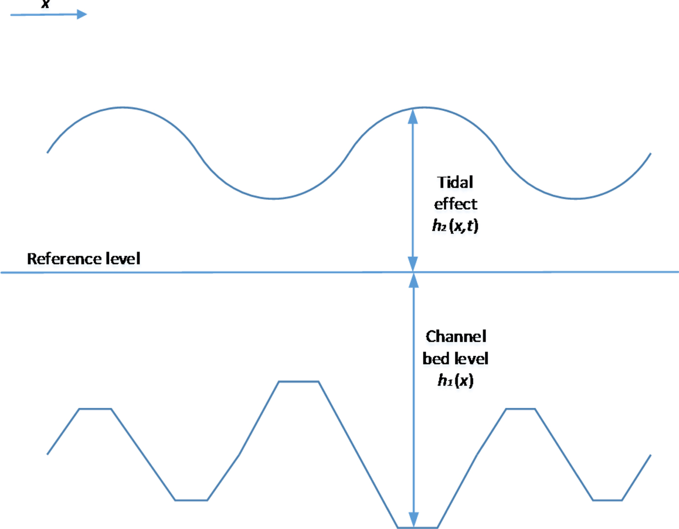
Figure 2. Components of water depth estimation.
2.1.1. Bathymetric profile of the navigable channel
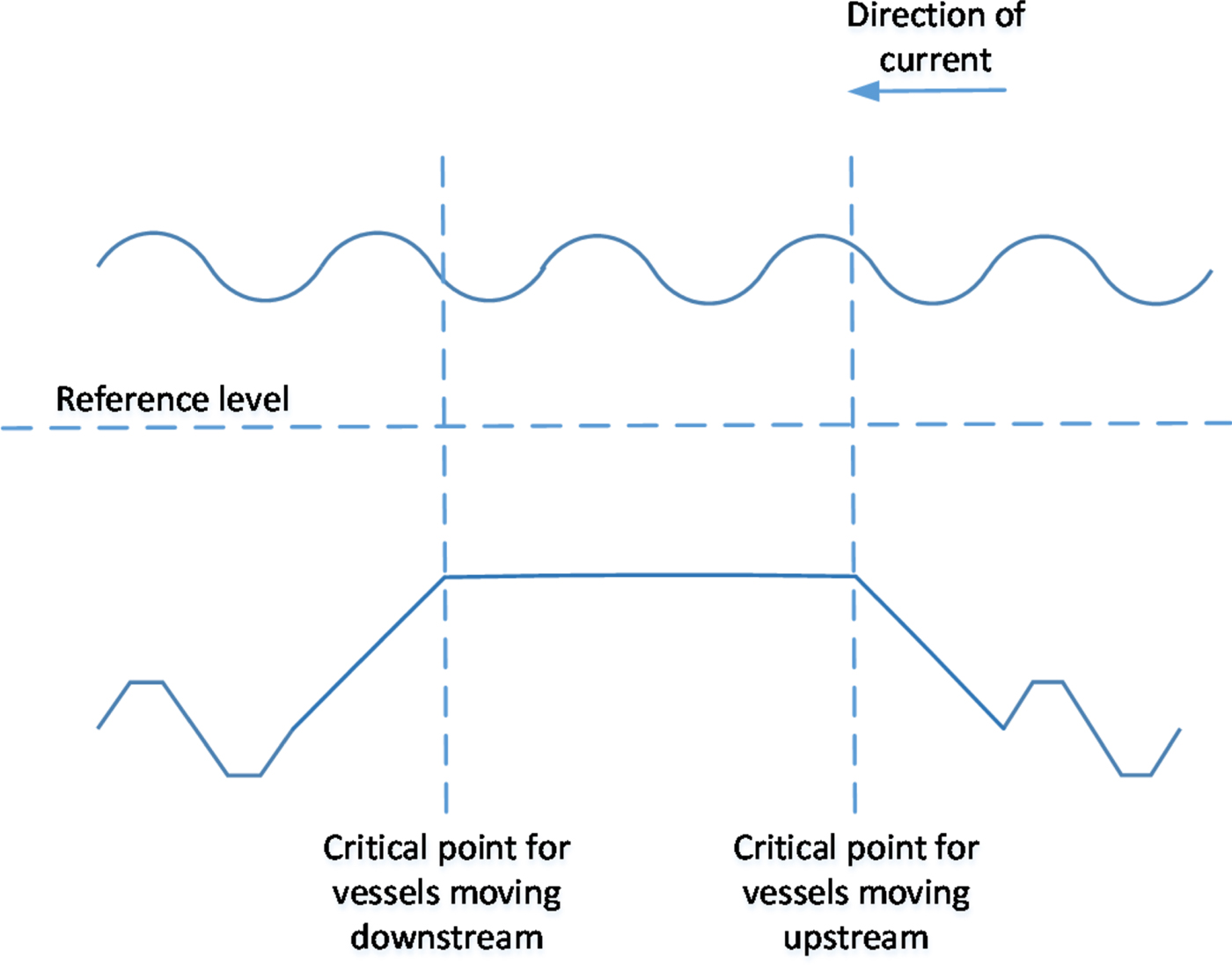
The first component of the maximum draught is the channel bed level, obtained from the bathymetric profile provided by the sonar scanning of the waterway bed along the navigable channel. The bathymetric profile allows us to determine the number and location of critical points, where the distance between the waterbed and the reference level is minimal. Figure 3 shows the layout of the 90 km Guadalquivir waterway leading from the Seville Port to the Atlantic Ocean, indicating all the independent bathymetry areas along the river, and Figure 4 represents the bathymetric profile of the navigable channel, with the critical points and anchoring areas identified. In the case of the Guadalquivir waterway, six critical points were identified as individual points on the longitudinal axis of the navigable channel, but the case may occur where the bathymetric profile presents a restrictive area or plateau instead of a single point. In this case, depicted in Figure 5, two critical points would be defined at both ends of the restrictive area: one for vessels moving upstream and the other one for vessels moving downstream. The rationale behind this is that any vessel crossing a critical point at any time should be able to continue navigating safely past that zone even on a falling tide. Anchoring areas, on the other hand, can, without loss of generality, be defined as points in the navigation channel where any given number of anchoring vessels can be hosted at any state of the tide.

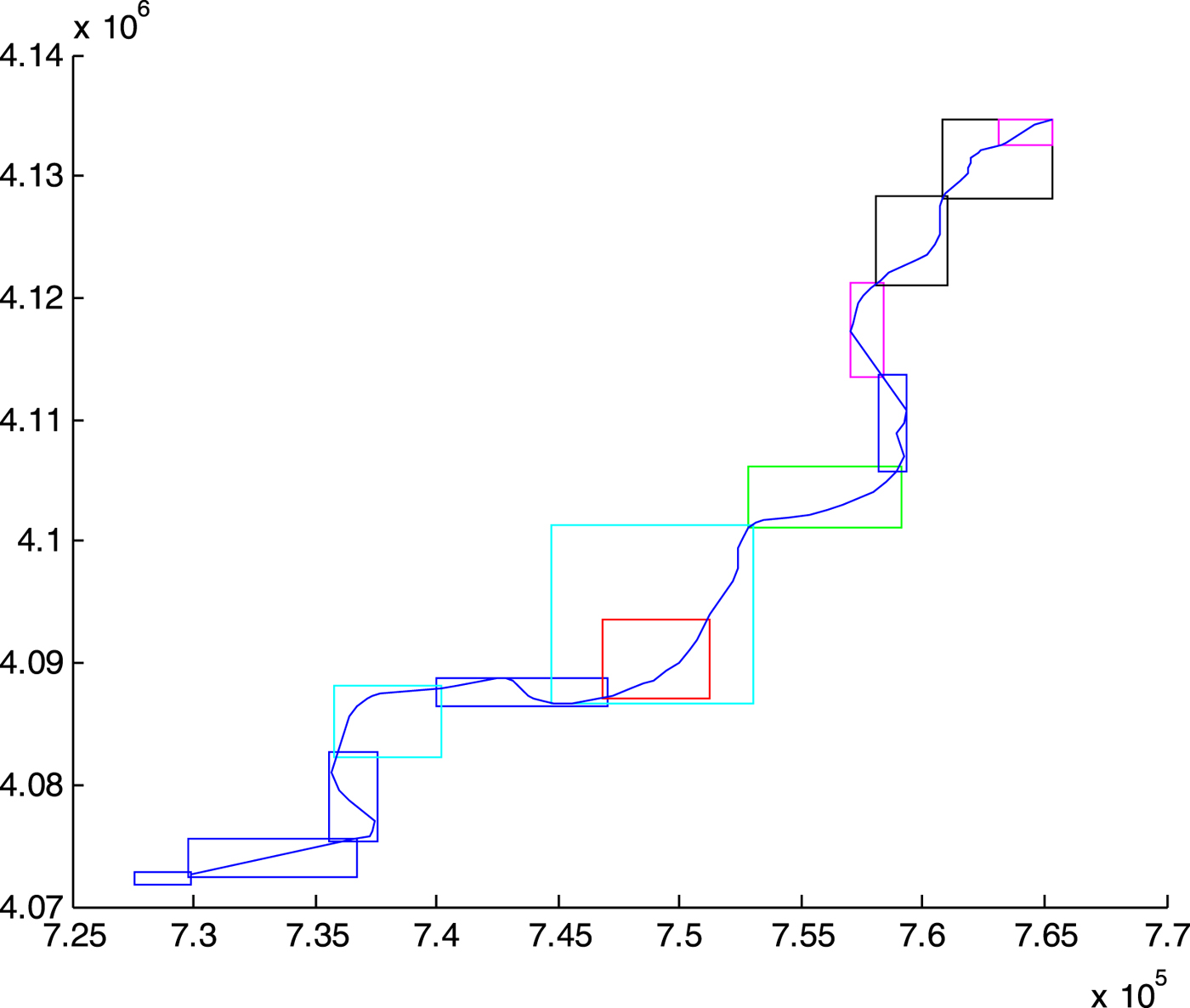
Figure 3. Layout of the Guadalquivir inland waterway, leading from the Seville Port (upper right hand) to the Atlantic Ocean (bottom left hand). This navigable waterway has a length of approximately 90 km (the coordinate values shown on the axes are expressed in metres).

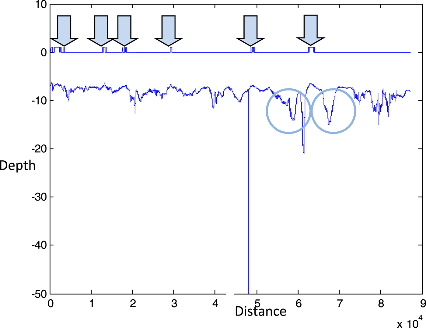
Figure 4. Bathymetric profile of the navigable channel along the Guadalquivir waterway, with the critical points marked by arrows and the anchoring areas by circles. The values on the axes are expressed in metres.

Figure 5. Definition of two critical points, one for upstream vessels and another for downstream vessels, in the event of a bottleneck plateau.
2.1.2. Effect of the tidal wave
The second component of the maximum draught estimation is the tidal wave forecast, which represents the dynamic component of the available water depth. This tidal wave may be estimated using a time series resulting from empirical samples and high- and low-tide hourly forecasts (Matte et al., Reference Matte, Jay and Zaron2013; Tamura et al., Reference Tamura, Bacopoulos, Wang, Hagen and Kubatko2014; Wei et al., Reference Wei, Yang, Song, Abbaspour and Xu2013), but in our case, it was obtained from the linear superimposition of harmonic functions with different frequency, amplitude and phase shift, calibrated with the data obtained from eight mareographs (see Figure 6) distributed along the waterway (Díez-Minguito et al., Reference Díez-Minguito, Baquerizo, Ortega-Sánchez, Navarro and Losada2012; Losada et al., Reference Losada, Díez-Minguito and Reyes-Merlo2017). Then, the tidal wave function h 2(x, t) at each critical point and anchoring area was obtained through linear interpolation between the two closest mareographs.

Figure 6. Location of mareographs along the Guadalquivir River.
The time-dependent available water depth was then estimated as the sum of both magnitudes, the channel bed level h 1(x) and the tidal wave h 2(x, t). Figure 7 shows an example of real-time available depth for the two anchoring areas and the six critical points distributed along the Guadalquivir waterway. The maximum draught for navigation was then determined by subtracting the under-keel clearance c i from this available depth for each vessel i.

Figure 7. Real-time available depth for the two anchoring areas (in blue circles) and the six critical points of the Guadalquivir waterway. The vertical axis is expressed in metres and the horizontal axis in 15-minute intervals.
2.2. Determination of vessel time windows
This second step of the procedure follows the estimation of the maximum draught h i(x j, t) for each vessel i at the different critical navigation points j along the waterway, and seeks to determine the time intervals during which each vessel may navigate through each critical point. The time windows through individual critical points then allow us to calculate the overall feasible intervals for each vessel along the whole waterway, which are determined by passing through the most restrictive critical point.
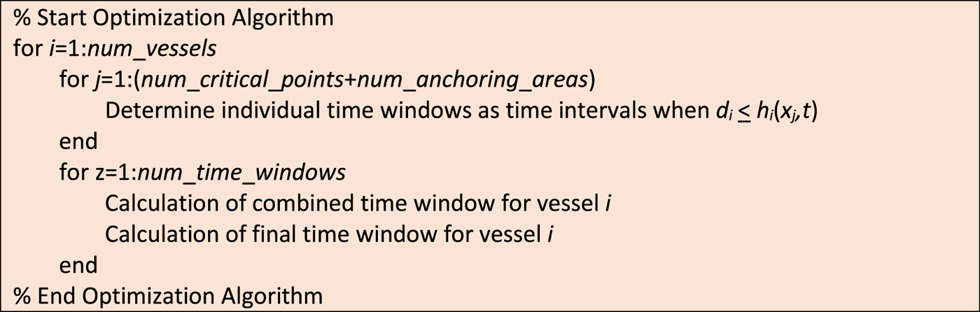
The main parameters for this module are the number of vessels to schedule (num_vessels), the number of critical points along the waterway (num_critical_points) and kilometre mark of each one, and the number of anchoring areas along the waterway (num_anchoring_areas) and kilometre mark of each one. Additionally, the data needed for each vessel i includes its Estimated Time of Arrival (ETA i) or Departure (ETD i), depending on whether the vessel is travelling upstream or downstream, and its draught d i and average speed v i. The algorithm (see Figure 8) starts with the determination of the individual navigation time windows [it ije, it ijl] for each vessel i through each critical point j. Specifically, the calculations are as follows:

Figure 8. Basic pseudo-code for the optimisation algorithm.
 $$\eqalign{{it}_{ije} &=t\ \hbox{when}\ d_{i}=h_{i}(x_{j},t)\ \hbox{and}\ h_{2}(x_{j},t) > h_{2}(x_{j},t-1) \cr {it}_{ijl} &=t\ \hbox{when}\ d_{i}=h_{i}(x_{j},t)\ \hbox{and}\ h_{2}(x_{j},t) < h_{2}(x_{j},t-1)}$$
Since the planning horizon comprises several tide cycles (we included four tide cycles in the planning horizon for our Guadalquivir River calculations), each vessel is likely to have more than one time window for each critical point, typically one per cycle. The number of individual time windows thus obtained for each vessel is num_time_windows. Once the individual time windows are calculated, they are used to determine the combined time window [ct ije, ct ijl] for each vessel i and critical point j. These combined time windows correspond to the time intervals during which each vessel needs to pass through each critical point in order to guarantee that it will complete its navigation process passing also though all the other critical points within the determined time windows. The determination of these time windows is carried out in a backtracking sequence, described in Figure 9, where num_points = num_critical_points + num_anchoring_areas + 2 (to include the two points corresponding to the river mouth and the port entry gate). In this sequence, vessel_direction can be either “upstream” or “downstream”, and the calculation of time windows is different for each case.

Figure 9. Pseudo-code for the procedure implemented to determine the combined time windows, both for upstream and downstream vessels.
We have illustrated the operation of the algorithm with the example shown in Figure 10, corresponding to a vessel traveling downstream through a waterway with two Critical Points (CP). Assume the individual time window for the vessel in CP1 is [4·5, 13·8], and [3, 8·8] in CP2. Then, calculations for CP1 indicate that, in order to pass CP1 between 4·5 and 13·8, the vessel must leave the port between 4·4 and 13·7 (displaced lower and upper bound), and will then pass CP2 between 6·7 and 16·0 and reach the ocean between 7·5 and 16·8. On the other hand, calculations for CP2 indicate that, in order to pass CP2 between 3 and 8·8, the vessel must leave the port between 0·7 and 6·5 and pass CP1 between 0·8 and 6·6. It would then reach the ocean between 3·8 and 9·6. Then, the combined time windows for the vessel for the start and end of its waterway navigation and for each CP are determined using the most restrictive values in each case, that is, the latest start (or largest displaced lower bound) and the earliest finish (or smallest displaced upper bound) of the different time windows.
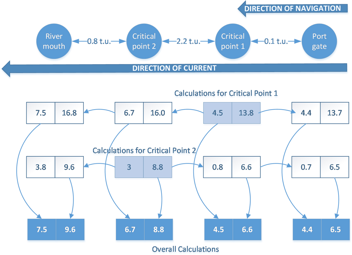
Figure 10. Example of determination of combined vessel time windows (t.u. = time units).
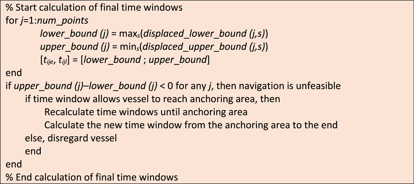
Finally, the combined time windows are modified if necessary when vessels cannot complete their journey through the waterway due to insufficient water depth, and are forced to anchor in one of the pre-specified areas and wait for the next tide rise. Should this happen (see Figure 11), the algorithm dissects the journey in two parts, one from the origin to the anchoring area and another one from there to the destination, and recalculates the time windows for each part. This is not habitual for vessels navigating upstream on the Guadalquivir waterway, since they move along with the tidal wave at a similar speed, but may happen when moving downstream, when they may run out of water depth before reaching the ocean.

Figure 11. Pseudo-code for the procedure implemented to determine the final time windows.
After this routine is concluded, the final time windows [t ije, t ijl] for each vessel i and critical point j are defined.
2.3. Multi-criteria fitness evaluation
Before moving on to how the different navigation sequences are generated, this section describes how they are evaluated, determining a level of fitness for each sequence. The decision on what should be the objective function to evaluate the result of the planning process is an essential step in the procedure (Ivančić et al., Reference Ivančić, Kasum and Pavič2013), given that this evaluation could be based either on time, on fuel consumption, on overall cost, or on a combination of several criteria, etc. In our case, due to the complex characteristics of inland navigation through a tidal waterway, we incorporated a multi-criteria objective function, whereby the best schedule will be the one with the smallest fitness value, which includes four different aspects:
Number of vessels included in the schedule (incl_vessels): if the procedure cannot find a feasible solution that contemplates all the active vessels it will leave one or more unscheduled, which should be penalised in the evaluation.
Waterway occupation time (occ_time): a schedule is better when the time elapsing since the first vessel in the sequence enters the waterway until the last one leaves it is as small as possible. The occupation time is determined as the time difference between those two events, calculated using the function DateNumber in Matlab\textsuperscript\textregistered. Thus, a total occupation time adding up to several hours is required for occ_time to take value 1 or higher.
Vessel waiting time (wait_time): also calculated using DateNumber, this criterion corresponds to the sum of differences between the ETA or ETD of each vessel and the time they enter the waterway to start their journey.
Number of overtaking and crossing operations (num_over): these operations entail a certain level of risk, and thus for safety reasons a schedule is better when it contains less of them. This normally means that faster vessels should be scheduled first.
The evaluation process also considers specifically the number of oversized vessels that are excluded in the solution (excl_oversize). These vessels, which due to their size cannot cross or be overtaken by others while in the waterway, result in a strong tendency of the sequencing algorithm to leave them unscheduled, when they often happen to be the most relevant or profitable ones for the port. Taking all the above into account, the objective function is as follows:
 $$\eqalign{{Fitness} &= w_{1}\cdot incl{\_}vessels + w_{2} \cdot occ{\_}time + w_{3} \cdot wait{\_}time \cr &\quad + w_{4} \cdot num{\_}over + w_{5} \cdot excl{\_}oversize}$$
where w i are the weights associated to each criterion, which need to be calibrated by the planner. Section 3 contains a description of the calibration experiments we carried out, and the justification for the weight values we selected for the application of the procedure in the Seville Port.
2.4. Proposed optimisation routine
The proposed optimisation routine used to optimise the vessel sequence along the waterway uses four new parameters in the analysis:
The number of vessels that need to travel upstream, from the ocean to the port (num_up)
The number of vessels that need to travel downstream, from the port to the ocean (num_down)
The number of oversized vessels (num_oversize)
The maximum number of vessels to use as a threshold in the exhaustive search process (max_num)
Using this data plus the time window information already calculated, our procedure works with four possible alternatives:
a) If num_up + num_down < max_num, the algorithm carries out an exhaustive search with all the possible combinations, and returns the best one. The number of possible combinations is (num_up + num_down)!
b) If num_up + num_down > max_num but num_oversize =0, num_up < max_num and num_down < max_num, then both directions (upstream and downstream) are planned independently with the same type of exhaustive search.
c) If num_up + num_down > max_num and num_oversize =0, but num_up > max_num and/or num_down > max_num, then each direction is planned independently, and the vessels going in each direction are clustered according to their ETAs or ETDs in a divide-and-conquer procedure (Smith, Reference Smith1985). Each cluster should contain an equal, or as equal as possible, number of vessels, smaller than max_num. Then, each cluster is sequenced with an exhaustive search analysis.
d) If num_up + num_down > max_num and num_oversize >0, then both directions need to be planned jointly (as oversized vessels impede crossings). Vessels are clustered according to their ETAs and ETDs (allowing both upstream and downstream vessels inside each cluster), and each cluster is then sequenced with an exhaustive search analysis.
When evaluating each vessel sequence, the procedure assigns each vessel the earliest possible starting time for its journey, depending on its time windows. Despite the application of exhaustive search techniques, this procedure does not guarantee the optimality of the final solution, but the tests we have carried out show significant improvements with respect to other alternative techniques, as described in Section 3.
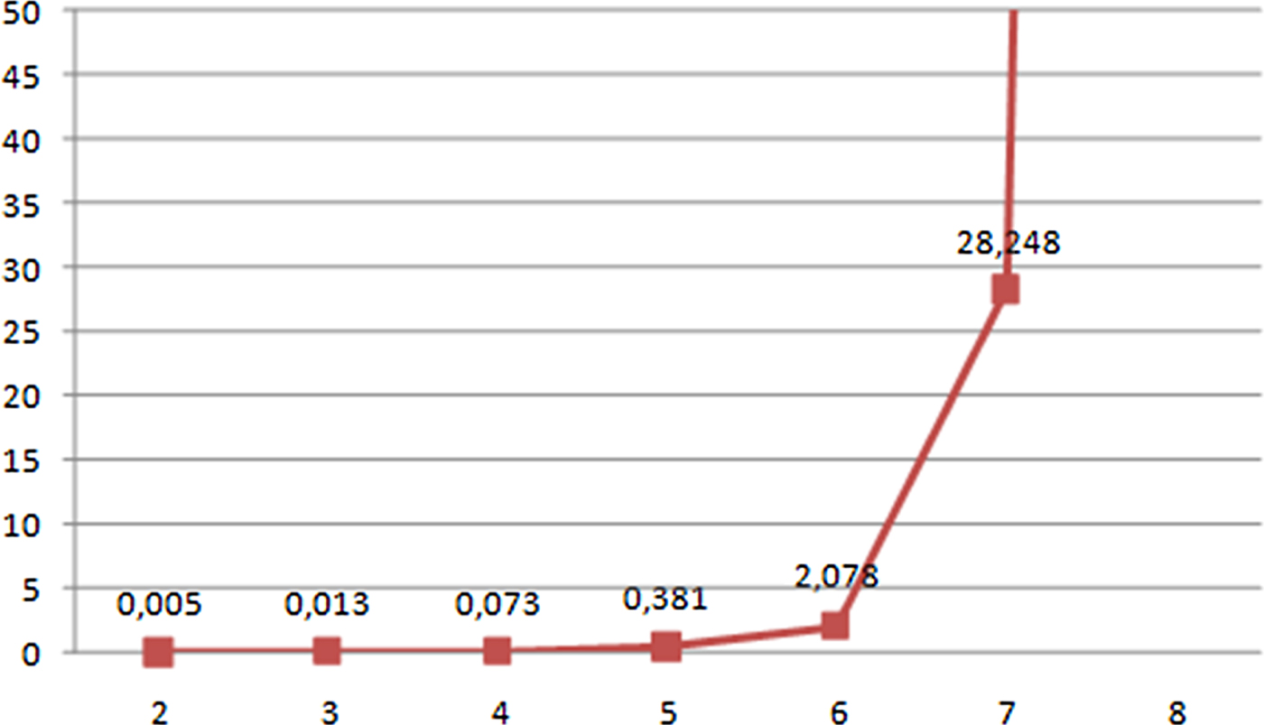
On the other hand, the computational time required to build a navigation plan based on exhaustive search depends on the number of vessels involved, but the experiments carried out have shown how this computational time remains relatively low (for a navigation planning problem) until a certain threshold number of vessels is reached and then increases rapidly. This number of vessels should provide the value for the max_num parameter. Figure 12 shows the time required to solve an exhaustive search procedure on the Guadalquivir River depending on the number of vessels involved, which explains why our chosen threshold value for max_num was equal to six. This keeps the overall computational time reasonably low (see Table 3), which also allows for recalculations, in case the planner wants to test different alternative solutions with different weight values, or in case new vessels are dynamically added to the system due to unforeseen navigation requests.

Figure 12. Computational time (expressed in minutes) required to complete an exhaustive search on the Guadalquivir River depending on the number of vessels involved.
2.5. Management of crossing and overtaking operations
Once the navigation plan has been determined, the procedure ends with the identification of problematic overtaking or crossing operations between vessels. Due to the bends or width variations in the navigation channel, some areas are not appropriate for these operations; these areas must be located in advance, and identified by their beginning and end kilometre points on the longitudinal axis of the navigation channel.
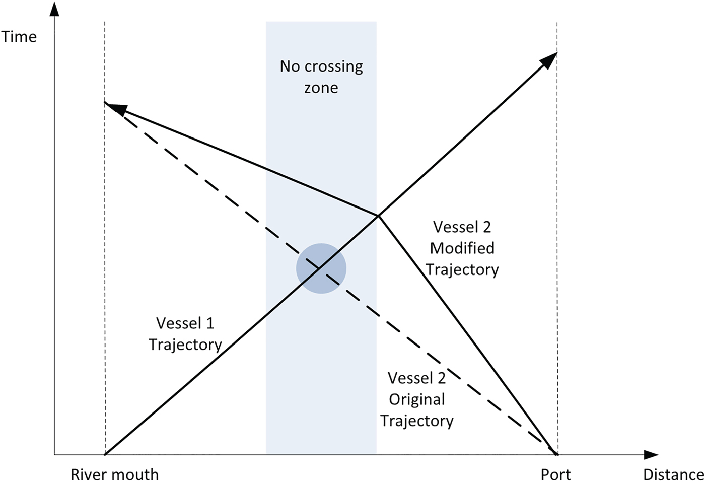
Figure 13 shows an example of this type of situation, with two vessels, one traveling upstream and the other downstream, expected to meet inside a no-crossing zone. In that case, the plan for the lighter of the two vessels will undergo a modification consisting of slightly increasing or reducing its speed in order to cross the other vessel outside the zone. The same operation would be carried out in the case of an overtaking manoeuvre.

Figure 13. Example of modified navigation plan due to the existence of a vessel crossing in an inappropriate zone.
3. APPLICATION RESULTS
This section contains the validation of our optimisation procedure through its application on one hand to a series of real problems taken from actual operation days at the Seville port and on the other hand to several test problems whose conditions are complicated through the introduction of an unusually large number of vessels. When solving these problems, we compared the results returned by our proposed optimisation routine with other techniques, including the ETA/ETD-based sequence, where vessels are sequenced on a first-come, first-served basis; the size-based sequence, where vessels are scheduled in ascending order of their size to benefit from the rising of the tide; and an adaptation of the savings algorithm (Clarke and Wright, Reference Clarke and Wright1964).
For the validation experiments, we assumed a five-minute minimum safety distance between vessels, and the weight values w i for the computation of the multi-criteria objective function were determined by a calibration routine where four weight scenarios were tested (see Table 1). The first scenario does not privilege any criterion, and in the second one the exclusion of oversized vessels is heavily penalised, which is equivalent to a soft constraint (Rossi et al., Reference Rossi, Van Beek and Walsh2006). The third scenario is safety-oriented, with larger weights allocated to the number of overtaking and crossing operations and, to a lesser degree, to the waterway occupation resulting from the navigation plan. Finally, the fourth scenario is efficiency-oriented, where the focus is instead on the number of vessels included in the plan and their waiting times.
Table 1. Weight scenarios contemplated in the calibration tests.
Table 2 shows the results of one of the calibration tests, with four vessels (one of them oversized) moving upstream and two moving downstream, where the differences between the four weight scenarios are evident. In the first one, with equal weights, the oversized vessel is excluded from the navigation plan, which does not happen in the second one, where this type of exclusion is directly penalised. The safety-oriented scenario returns no crossing or overtaking operations and a reduced value for the waterway occupation time, but this happened because only one vessel was included in the navigation plan. On the other hand, the efficiency-oriented set of weights included as many as four vessels with a reduced overall waiting time, but causing one crossing operation and occupying the waterway for many hours.
Table 2. Results obtained from the calibration example with four vessels moving upstream, one of them oversized, and two moving downstream.

The optimisation tool installed at the Seville Port Authority is fully configurable, so the planner can test several different weight options before choosing the definitive navigation plan. In any case, after analysing the results of the calibration tests, our recommendation was to use the second weight scenario to plan daily operations. We have used this combination of weights hereafter, to solve the set of real and test problems and compare the results provided by our procedure with other optimisation techniques. The description of the problem set, including the computational time required in each case by our algorithm, is shown in Table 3, and Table 4 contains a comparison of the results.
Table 3. Description of the set of validation problems, including the computational time required by our algorithm to solve each one of them.
Table 4. Comparison of results obtained for the validation problems using four different sequencing techniques. The sequence with best fitness value obtained for each problem is marked in bold.

These tables show that the exhaustive search sequence always obtains the best results, even when the number of vessels is high and they have to be clustered. In the real operation scenarios (1-24), the savings algorithm almost always equals the best solution found, in a similar computational time. With respect to the time- and size-based heuristics, their computational times are always less than one second, but the quality of the solutions is usually worse: the size-based sequence (traditionally used at the Seville Port) only equals the best solution in nine scenarios, and the ETA/ETD-based sequence in 11. On the other hand, the exhaustive search procedure clearly outperforms the other heuristics in the larger test scenarios (25-30), both in terms of computational times (with respect to the savings algorithm) and of solution quality.
As a result, our proposed procedure, based on exhaustive search, has proved the best alternative for the optimisation of navigation plans on the Guadalquivir River, both in terms of solution quality and computational time, obtaining the best solution for all the problem instances in typically less than a minute, even for the larger instances where the problem has to be partitioned as described in Section 2.4.
4. CONCLUSIONS
The sequencing of vessels for navigation along a tidal waterway is a complex problem influenced by many aspects: bathymetric profile of the waterway, characteristics of the tidal wave, size and speed of the vessels, arrival and departure times, etc. Also, there is not a single criterion with respect to which the best navigation sequence can be determined. We have described a multi-criteria procedure to design that sequence, considering the number of vessels included in the schedule, the waterway occupation and waiting times, and the level of safety measured as the number of dangerous operations expected. The sequence is determined by means of an exhaustive search procedure, even if the number of vessels to schedule is very high and they should be previously clustered according to their estimated arrival and departure times.
The application of the procedure to a series of real and test problems in the Seville Port has proved that the above methodology constitutes an efficient decision-support system for navigation planning. The system is currently running at the port, increasing the efficiency of navigation plans and significantly reducing the operator time required to build them. In any case, the system is flexible enough to be used in any tidal waterway, ensuring smooth operations with a high level of safety. Nevertheless, future research directions should contemplate the integration of waterway navigation with other port scheduling problems, such as the allocation of berths or the operation of pilots, cranes or stowage crews.
ACKNOWLEDGMENTS
The authors wish to acknowledge the financial support of projects Tecnoport2025 (Ref. FIUS-2284) and Ecotransit (Ref. TEC2013-47286-C3-3-R) for the completion of this work. We also thank the three anonymous reviewers for their constructive and rigorous comments.