
Informal institutions are ‘socially shared rules, usually unwritten, that are created, communicated, and enforced outside of officially sanctioned channels’.Footnote 1 Our interest here is in the evolution of one particular informal institution, the study of which yields general methodological lessons for scholars of comparative politics: the rule that in Westminster systems, the ‘Shadow Cabinet’ – the group of frontbench spokespersons from the official opposition – forms the executive when the party currently in opposition next enters government. This relationship is at the core of Westminster democracy for reasons that are obvious from any textbook account of those systems.Footnote 2 Yet it has never been part of statute law, and was not always the case in practice: in the eighteenth and early nineteenth centuries, leaders of governments (prime ministers) were implicitly or explicitly selected directly by the crown,Footnote 3 and later by some decision-making process within the majority party.Footnote 4 Prior to modern times, the presence of competing formal and informal institutions meant that conflicts over exactly which set of rules and actors had precedence were common.Footnote 5
In modern Westminster systems, where partisan voting is the normFootnote 6 and majoritarian electoral systems deliver disproportionate government numerical superiority in parliament,Footnote 7 along with disciplined backbenchers,Footnote 8 the leadership of the winning party can expect comparatively long durations in government, and the ability to propose and enact legislation close to its ideal point.Footnote 9 Thus the identity of the government in waiting, and the fact that it will become the executive once in office, has profound implications for almost all actors in the system, including voters and legislators. This is quite apart from other significant roles that the Shadow Cabinet plays: inter alia, organizing opposition to the government’s legislative plans in the division lobbies,Footnote 10 holding ministers to account in debates,Footnote 11 and providing a formal link between the parliamentary party and its grassroots.Footnote 12 Yet in stark contrast to the Cabinet,Footnote 13 and with exceptions,Footnote 14 there has been little work on the opposition per se. This is especially true in the literature on the origins and development of the Shadow Cabinet and the informal institution to which it is vital.
While competition for votes provides the incentive for the teams of current and would-be ministers to organize themselves into coherent party groups today, it is far from obvious that this was the original motivation for their formation. Indeed, the dominant explanation of the origins of the Cabinet – that of CoxFootnote 15 – focuses on the specifically procedural problems that the organization emerged to counteract: in particular, resolving a parliamentary ‘tragedy of the commons’ after the First Reform Act. Thus one plausible explanation for the evolution of the Shadow Cabinet is that it corrected some functional misfiring at the center of Westminster life, and did so in a way that improved the efficiency of the institution as a whole. In this sense, the emergence of the government in waiting is an endogenous process, and a response to other forces in parliament – rather than the direct product of some exogenous shock.Footnote 16 In contrast to such a theoretical position, scholars have been quick to recognize the importance of the Second Reform Act in ushering in a more modern period characterized by a ‘triumph of partisan politics’,Footnote 17 in which parties began to lay out more coherent ideological positions and turned to more disciplined, hierarchical organizational forms both insideFootnote 18 and outsideFootnote 19 Parliament. From this perspective, the Shadow Cabinet might be seen as the product of electoral forces unleashed after franchise extension: a strategy – or the consequences of a strategy – by which (opposition) Members of Parliament (MPs) could win working-class votes at the ballot box. That is, the Shadow Cabinet is the product of a competition problem, rather than a procedural problem.
At base, determining which of these theoretical positions is most plausible – or in what combination – requires us to accurately characterize the timing and nature of the emergence of the Shadow Cabinet. If it came into being in something approximating its modern form around the time of the rationalizations that CoxFootnote 20 describes – that is, shortly after the 1830s – we have evidence in line with a procedural theory. In stark contrast, if its emergence is clearly post-Second Reform Act (and to boot, relatively shortly after), we are on firmer ground with a competition story. Of course, the reality of historical change stretched out over a 100-year period of reform means that the researcher is rarely in a position to speak in absolutes: that one account is correct while the other is wrong. A more sensible strategy is thus to weigh the relative heft that might be given to the differing accounts.
With such an approach in mind, an immediate problem is that executing any large-n studies of informal institutions is extremely difficult,Footnote 21 not least because (almost by definition) they leave less of a paper trail of official documentation. In the specific case of the Shadow Cabinet, only in very recent times have its membership or activities been recorded for outside observers.Footnote 22 The result is that researchers must make more uncertain inferences about who, exactly, constitutes the body itself and what it is doing. This problem is compounded in Westminster systems by the fact that the opposition per se is procedurally weak and hard to observe in action: the usual metrics for examining the strength of opposition organization – like roll ratesFootnote 23 or the strategic use of committee controlFootnote 24 in the US Congress – are either very consistently zero or simply non-existent. Put more succinctly, since oppositions almost always lose against governments – in terms of what gets onto the legislative agenda and what becomes law – there is seemingly little variation in legislative output to explain or explore over time.Footnote 25 Consequently, studying the opposition and its role in informal institutions is extremely challenging.
Here we attempt to improve matters by describing informal institutions in a way that is familiar to political methodologists in comparative politics: by using a latent variable representation in which an observed variable for a given unit (speech contents) may be used to make inferences about an unobserved one (Shadow Cabinet management) and its relationship with an outcome of interest (Cabinet membership).Footnote 26 As suggested by this strategy, a second contribution below is to provide a text-as-data measurement strategyFootnote 27 using the almost one million utterances between the approximate dates of the First and Fourth Reform Acts (1832–1918) in which the relevant informal institution first emerged and then evolved. We model these speeches using a measure that considers the ‘burstiness’Footnote 28 of different (government and opposition) actors over time: specifically, we introduce a validated method for scoring individuals via their spoken contributions to debate in the House of Commons. This metric relies on the relative spike in activity around particular terms that MPs use, in order to measure members’ latent agenda-setting abilities. By comparing the estimated abilities of opposition members, we can infer when and how the Shadow Cabinet emerged and thus contribute to the debate about its origins sketched above.
We find that, while the First Reform Act made the Cabinet, the Second Reform Act made the Shadow Cabinet. More subtly, we provide theory and evidence to suggest that the 1867 Second Reform Act, and its associated introduction of a ‘party-orientated electorate’ (in the sense of CoxFootnote 29 ) was crucial for the establishment of a hierarchical opposition leadership, with small numbers of senior individuals increasingly dominating exchanges from the 1870s and 1880s onwards. We show that after the 1870s, (a) the opposition as a whole was able to wrestle back some noticeable control of the agenda from the Cabinet, (b) a small group of opposition individuals emerged who, relative to their co-partisan colleagues, increasingly dominated debates and (c) the relationship between being one of these individuals and taking a role in the next Cabinet controlled by their party was increasingly strong. In explaining these findings, we expend some effort to validate our measure and demonstrate its strength over potentially misleading alternatives. These steps help more evenly balance the literature on British political development – including the work on the export of its governance arrangementsFootnote 30 – by appropriately focusing on both government and its alternative.
SHADOW CABINET: LITERATURE AND ORIENTATION
Students of British political development typically focus on the period of profound transformation between the First (1832) and Fourth (1918) Reform Acts, and our study does the same. Discussion of changes in Parliament during this time can be found in many sources,Footnote 31 but several key developments are as follows: first, as per Cox,Footnote 32 the cabinet as the agenda setter emerged in the 1830s as an attempt to solve a common resource problem – too many MPs were taking up too much time with self-promoting minutiae – in the aftermath of the Great Reform Act. Secondly, as the century progressed, parties showed increasing cohesion in their division voting;Footnote 33 the period of the Corn LawsFootnote 34 and their immediate aftermath was one of unusual disunity and party realignment. Executive dominance was arguably complete in its modern sense with the coming of the ‘Railway Timetable’, introduced by Prime Minister Balfour in 1902,Footnote 35 which gave governments clear precedence to introduce (and pass) their legislation with little opportunity for the opposition to overturn such plans on the floor or division lobbies in the House of Commons.
Not least because it plays a larger role in policy making, and has done for a longer period, the Cabinet has attracted much more scholarly attention than its opposition counterpart. As noted, the CoxFootnote 36 account dominates and suggests that the emergence of the Cabinet as an organizational force, whatever its later expanded role in public policy, occurred as a solution to a procedural problem. A puzzle that arises from this accepted assertion is the timing and precise form of the Shadow Cabinet’s emergence as a de facto organization. On the one hand, we might expect it to (begin to) arise fairly soon after this, motivated perhaps by the sudden threat of institutional dominance by a powerful executive or, more charitably, stimulated by some other potential efficiency gain. This might include the requirement to provide swift and acceptable transitions of power after elections,Footnote 37 or to safeguard backbencher rights in general. Certainly, scholars of other Westminster institutional developments – like the advent of (aggressive) parliamentary questions – have made the case that they arose relatively quickly from non-Cabinet members’ need to keep the executive in check.Footnote 38 Similarly, certain institutional behaviors, such as cohesive division voting against the government’s legislation and the commensurate use of government whipping to make executive bills into parliamentary acts,Footnote 39 started not long after the rationalization noted by Cox.Footnote 40
On the other hand, historians suggest that the notion of the informal institution of government in waiting did not emerge until much later: after the Second Reform Act (1867). This suffrage expansion and the ‘triumph of partisan politics’Footnote 41 it induced was commensurate with a decline in personalized, patronage appeals.Footnote 42 An alternative argument, then, is that the Shadow Cabinet emerged as a collection of opposition leaders with specific designs on governmental roles, putting forth a more unified policy-based appeal than had been previously used in elections. Here, analysts have pointed to early campaigning efforts by Liberal leader William Gladstone in the late 1870s as the start of this process.Footnote 43 The observational implication of this position is that we should not see the evolution of an opposition leadership until after suffrage expanded.
While qualitative scholars have documented changes in how opposition leaders acted and, more broadly, how they strategized, they have not provided a systematic assessment of such claims. In particular, they have been unable – mostly due to data limitations – to link parliamentary activity to both opposition organization and subsequent government formation. Though we will shortly discuss our data-driven attempt to resolve this debate, two points of circumspection are worth making here. First, our ‘testing’ of the procedural vs. competition theory relies on relative timing after 1832. This is justifiable insofar as the most well-cited and widely accepted account – that of CoxFootnote 44 – portrays the Great Reform Act as the key impetus for the formation of the Cabinet, and that all other sources we have seen claim this institution predated the Shadow Cabinet.Footnote 45 A second, related, issue is that we assume that changes in the legislative and electoral environment take at least a little time to take effect on MP behavior. Naturally, such caveats mean that sharp inference is difficult, a position that we believe is philosophically in line with our comments above about the importance of a measured approach to weighing the evidence for the theories.
A Methodological Problem
As with much of Westminster constitution making, formal de jure recognition of entities with political power and importance has traditionally come much later (if at all) than their de facto existence as a force. Thus the informal practice by which a parliamentary opposition critiques the government has a long history: it was well underway by the 1720s, with the present-day term of the ‘His Majesty’s loyal Opposition’ first appearing in debate in 1826.Footnote 46 Turning to statute to characterize the hierarchical structure of the opposition is of little help – indeed, as with many other informal institutions at Westminster, it is only with respect to salary commitments that the leader of the opposition is mentioned in law.Footnote 47 The term Shadow Cabinet was used as early as the 1880s, though not with any legal basis, and it initially referred to a set of ex-ministers, now out of office as their party was no longer in government.Footnote 48 Initial meetings of the Shadow Cabinet were more informal than modern practice (and records of them are scant), but in the post-Second World War period in Britain, opposition parties gave chosen senior MPs specific policy responsibilities and titles with the expectation that they would fulfill a similar ministerial role should their party win a subsequent general election.Footnote 49 All told, there are few official records of opposition that we can call upon to answer our question of interest.
This problem is made harder still because, as alluded to above, oppositions – and Shadow Cabinets – are weak in procedural terms: Westminster governments are typically single party,Footnote 50 and face few serious institutional impediments to imposing their will.Footnote 51 A consequence is that the opposition rarely achieves legislative victories, and thus one cannot usefully measure outcomes that would be seen in other parliaments, such as roll rates, successful legislation sponsoringFootnote 52 or negative agenda control.Footnote 53 Since these measures take a value of (near) zero at Westminster, they cannot tell us much about who is organizing opposition to the government. Yet this is a key element of exploring the particular informal institution of interest here. What we do have is speeches, and we return to their use below.
Thinking in a more general way, informal institutions are difficult to analyze because they are rules that connote probabilistic statistical relationships between inputs (X) and outcomes (Y), but for which X and/or Y are not directly observable.Footnote 54 Typically, when faced with a latent variable that is an important part of a data-generating process (as X is here), political methodologists in comparative politics attempt to infer its values from other, observed variables.Footnote 55 To keep matters simple, suppose that there is one such observed variable, denoted Z, and that for the units in the study, their (latent) value of X probabilistically determines their (observed) value of Z, but that Z has no direct relationship with Y itself. In what follows, we will take precisely the route implied by our comments about X, Y and Z. For us, Y is the status of an MP as part of the Cabinet in a particular time period. This is observable. Meanwhile, X is his/her status (or not) as a member of the Shadow Cabinet in the prior parliament, which occurs prior to Y. For our period, this is latent, and cannot be directly observed. Below, Z will be an MP’s agenda-setting ability, derived from observational data on his/her speeches via a particular metric that we will define in some detail. Thus an MP’s speeches will help us infer whether he/she was a member of the Shadow Cabinet (along with other details on the Shadow Cabinet’s evolution), and we will then study the relationship between this shadow status and promotion to the Cabinet once his/her party is in power. In this way, we can assess the changing nature of an informal institution that is vital to the functioning of Westminster democracy.
DATA
The data we use are described in Eggers and Spirling,Footnote 56 but the essence is this: we have access to 856,405 House of Commons speeches recorded by Hansard between 1832 and 1915.Footnote 57 Each speaker has been identified, which in turn has been matched to a unique MP identity. Other information pertaining to these MPs includes their party affiliation in any given parliament, along with their ministerial service record. The speech records are machine readable, and can be processed using software tools discussed below.
For our purposes, the speeches are organized by parliamentary session, a period with a mean length of around 200 days. The period between two general elections (usually comprising several sessions, each starting about a year apart) is referred to as a parliament. We obtained dates for the sessions from the usual sources for the period: Cook and Keith and Butler and Butler.Footnote 58 Thus for any given day, we know the identity of the government and opposition parties, and thus any contemporary MPs. In what follows, we will limit our analysis to MPs running in general elections under either a Conservative or Liberal label (as originally demarcated by Craig, Craig and Walker),Footnote 59 the two parties that held ministerial positions during this time, and thus for whom the concept Shadow Cabinet makes the most sense.Footnote 60
As a quick overview of the general trends in our data, consider Figures 1 and 2. Figure 1 reports the number of government (top panel) and opposition (bottom panel) MPs in our data over time (note that the total membership of the Commons is essentially constant: around 650–70 MPs). The solid line in both plots reports (on the right y-axis) the total number of speeches given by the government and opposition. It can be seen that the number of government MPs is approximately constant over time (at around 350), while the total number of opposition MPs falls slightly (in part owing to other – that is, non-Conservative, non-Liberal – opposition parties entering the fray). Meanwhile, the total number of speeches by government MPs rises after around 1880, reaching a peak toward the end of the data of around 16,000 speeches for the session. The total number of opposition speeches also increases very slightly over time, similarly peaking at the turn of the twentieth century.

Fig. 1 Summary of data: number of government party MPs and the number of speeches they made (top panel) and number of opposition MPs and speeches they made (bottom panel). Note: points refer to the left y-axis and are MP numbers; the solid line(s) are numbers of speeches for which the y-axis is to the right of the plots. In the top (bottom) plot, square points connote the Liberals (Conservatives) in government; round points connote the Conservatives (Liberals) in government.

Fig. 2 Summary of data: points are number of words per speech in the House of Commons (left axis); line is number of speeches per MP (right axis). Note: round points connote Conservatives in government; square points connote Liberals in government.
Figure 2 reports (on the left axis) the mean number of words per speech over time, while the right y-axis gives the mean number of speeches per MP during the period under study. We see a secular fall in the average length of speeches from a high of around 600 words to around 200. By contrast, the number of speeches given per MP rises both in mean and variance terms, and reaches a peak at the end of the data.
The patterns seen in the plots are evidence of a general tightening of executive control over proceedings in the House of Commons, and the expectation that more speeches would be questions or answers to those questions.Footnote 61 This trend of focusing on government business was joined by powers given to the House in the 1880s (in the face of Irish obstructionism) allowing it to ‘close’ debate, and speaker rulings that gave that officer a new ability to control overly long or irrelevant statements in the House. In the face of these changing control structures and totals, our approach below avoids absolute measures of opposition performance, instead comparing within oppositions and then in relative terms with respect to governments.Footnote 62
METHODS
While our X, membership of the Shadow Cabinet, is latent, we can observe members making speeches that can inform us about X via our observed variable Z. Each MP also has an observable set of covariates pertaining to their current role in the government (that is, Y) if they are part of the governing party. Our central concern is understanding which MPs ‘lead’ debate in parliament. Our strategy trades on the idea that influential individuals will raise concerns, terms, topics and issues that MPs will subsequently talk about in that and subsequent debates.Footnote 63
Concept and Measurement
One way to approach this measurement problem is to see speeches in the House of Commons as analogous to a stream of arriving data, the contents of which require modeling. In computer science, a popular way to examine such streams is to consider their ‘burstiness’, in the sense of Kleinberg.Footnote 64 The idea is to model the arrival times at which certain words – considered as a type of event – appear. Words that surge in use suddenly are said to ‘burst’ or to be ‘bursty’, which in practice means that they experience periods in which the typical gaps between occurrences become much shorter than is usual for that word. Depending on the nature of the stream process, there are different statistical models that may be fit to the data to determine burstiness.
When data arrive as a continuous process – rather than as, say, batches every year – KleinbergFootnote
65
suggests an ‘infinite-state model’ in which bursts are state transitions in a hidden Markov process. For a given term, we begin with a ‘base rate’ calculated as
 $${n \over T}$$
, where n is the number of speeches that uses a particular word and T is the total number of speeches in the session. Thus if there were 100 mentions of the term ‘boundary’ and 10,000 speeches, the base rate is
$${n \over T}$$
, where n is the number of speeches that uses a particular word and T is the total number of speeches in the session. Thus if there were 100 mentions of the term ‘boundary’ and 10,000 speeches, the base rate is
 $$\alpha _{0} \,{\equals}\,{{100} \over {10,000}}{\equals}\,0.01$$
, corresponding to a mean wait time of
$$\alpha _{0} \,{\equals}\,{{100} \over {10,000}}{\equals}\,0.01$$
, corresponding to a mean wait time of
 $${1 \over {0.01}}\,{\equals}\,100$$
speeches.Footnote
66
With the base rate in mind, we ask how the gaps between occurrences of the relevant term are changing as the session unfolds. In particular, the Markov process assumes that when in state i, gap times, x, are exponentially distributed with pdf
$${1 \over {0.01}}\,{\equals}\,100$$
speeches.Footnote
66
With the base rate in mind, we ask how the gaps between occurrences of the relevant term are changing as the session unfolds. In particular, the Markov process assumes that when in state i, gap times, x, are exponentially distributed with pdf
 $$f(x)\,{\equals}\,\alpha _{i} e^{{{\minus}\alpha _{i} x}} $$
where
$$f(x)\,{\equals}\,\alpha _{i} e^{{{\minus}\alpha _{i} x}} $$
where
 $$\alpha _{i} $$
is the rate, such that larger values of α imply smaller expected values for the wait time (
$$\alpha _{i} $$
is the rate, such that larger values of α imply smaller expected values for the wait time (
 $${1 \over \alpha }$$
) until the next event occurs.
$${1 \over \alpha }$$
) until the next event occurs.
Setting up the estimation problem continues by making
 $$\alpha _{i} \,{\equals}\,{n \over T}s^{i} $$
, meaning that the rate is proportional to a quantity s
i
. In keeping with the original KleinbergFootnote
67
presentation, s will be fixed at 2 for our purposes but i will be estimated as an integer greater than or equal to 1, and will be different at different times for the same word (depending on the state of the system). Put very crudely, the idea is to observe the series of gaps between uses of a term, and then to find values of i that (when plugged into the previous formula) will fit the data, with respect to the (exponentially distributed) wait times that were seen in practice. To see how this might work, and remembering that s is fixed, suppose we saw wait times of 20,20,10,5,10…. We can see that the third wait time (10) is half of the second (20), implying an increased value of i. Similarly, the fourth wait time (5) is half the previous one, implying that i has increased even further. The fifth wait time (10) suggests that i has declined, since the wait time has doubled. We will ultimately have a series of ‘states’ that describes our data, which is simply the vector of i values that we estimated.
$$\alpha _{i} \,{\equals}\,{n \over T}s^{i} $$
, meaning that the rate is proportional to a quantity s
i
. In keeping with the original KleinbergFootnote
67
presentation, s will be fixed at 2 for our purposes but i will be estimated as an integer greater than or equal to 1, and will be different at different times for the same word (depending on the state of the system). Put very crudely, the idea is to observe the series of gaps between uses of a term, and then to find values of i that (when plugged into the previous formula) will fit the data, with respect to the (exponentially distributed) wait times that were seen in practice. To see how this might work, and remembering that s is fixed, suppose we saw wait times of 20,20,10,5,10…. We can see that the third wait time (10) is half of the second (20), implying an increased value of i. Similarly, the fourth wait time (5) is half the previous one, implying that i has increased even further. The fifth wait time (10) suggests that i has declined, since the wait time has doubled. We will ultimately have a series of ‘states’ that describes our data, which is simply the vector of i values that we estimated.
To reiterate, i is the exponent of s: for a fixed s=2, an increasing i means that a geometric decrease must have been seen in wait times: that is, to go from our base rate model to s 1 to s 2 to s 3 requires at least a halving of the gap (and more than a halving if s were chosen to be larger than 2). Clearly, there will be a great many terms that never exhibit any bursts (they are ‘not bursty’) because their arrival rate is simply too uniform. Thus if the term ‘bill’ occurs exactly every 100 speeches, then the gaps between observations are not changing. As a result, the term exhibits no bursts in use. This logic potentially extends to any word, no matter how common. For example, the word ‘the’ might be used uniformly in every speech, and thus will demonstrate no bursts. In this case, the base rate, which is very high, will be a perfectly adequate model for the data.
This process has a second component: a cost term, denoted as γ, which essentially imposes a penalty when the system seems to move ‘up’ in intensity in terms of the underlying rate – no cost is imposed for the system to move down in intensity.Footnote 68 A larger γ is associated with relatively few upward transitions. Meanwhile, the exponential component (determined by s) encourages fitting a model to the data that reflects the actual sequence of gaps observed. The resulting minimization problem takes both parts into account, and thus attempts to fit the data with as few transitions as possible. Note that the bursts in this model are nested: that is, bursts of higher intensity occur within periods of lower-intensity activity. As per the original presentation, γ is set to 1 for our work here.Footnote 69
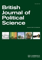
Conceived in the usual way, burstiness is a property of streams of events. One example is words in speeches (or MPs in debates, as explained below). We can, for example, examine the burst pertaining to the word ‘Ireland’ or ‘boundary’, and in Figure 3 we picture the latter of these terms for the 1884 session in which the Redistribution of Seats Act – which dealt with the redrawing of districts – was discussed: note the levels (literally, the states of the Markov process – the exponential distributions delivering the gap times – where 0 is the base rate) of the bursts that the word went through, and the varying lengths of those bursty episodes. In principle, we can do this for every term and every session.
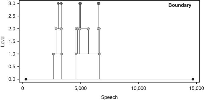
Fig. 3 Burst levels and burst durations for the word ‘boundary’ in the final session of the 1880 parliament (1884).Note: burst levels indicate the state of the Markov process at that point.
Our innovation is now to use these burstiness estimates to compare MPs with each other. To do that, we need a metric that allows us to compute a score for each member, taking into account the relative burstiness of their contributions. For us, this is a weighted sum. For each MP, a burst that begins with a speech made by him or her is scored as the length of that burst (literally, the number of speeches that occur while at the particular value of i) multiplied by its intensity. All such bursts are then summed into a total score. For example, consider an MP who made 100 speeches. Suppose that a word from one of these speeches launches a burst of intensity level 2 for a time period of 30, and a different word from the same speech launches a burst of intensity level 3 for a time period of 4. Meanwhile, a word from another speech launches a burst of intensity level 3 for a time period of 5. The overall burstiness is thus calculated as
 $$(2{\times}30){\plus}(3{\times}4){\plus}(3{\times}5)\,{\equals}\,87$$
. Note that bursts are hierarchical: a burst of level n can only occur within a burst of level m, where m < n. A consequence is that MPs cannot be given ‘credit’ for decreasing the intensity with which a particular word is used relative to the current period in which they are speaking. Note further that, if one MP boosts a term’s use to level 2, while a second MP boosts it further to level 3, the first MP receives ‘credit’ only for the level 2 burst, while the second receives credit only for the level 3 burst. This is simply a measurement strategy that accords with our notion of MPs building on the points of others; our metric thus rewards MPs who introduce terms, topics or ideas that subsequent speakers take up.
$$(2{\times}30){\plus}(3{\times}4){\plus}(3{\times}5)\,{\equals}\,87$$
. Note that bursts are hierarchical: a burst of level n can only occur within a burst of level m, where m < n. A consequence is that MPs cannot be given ‘credit’ for decreasing the intensity with which a particular word is used relative to the current period in which they are speaking. Note further that, if one MP boosts a term’s use to level 2, while a second MP boosts it further to level 3, the first MP receives ‘credit’ only for the level 2 burst, while the second receives credit only for the level 3 burst. This is simply a measurement strategy that accords with our notion of MPs building on the points of others; our metric thus rewards MPs who introduce terms, topics or ideas that subsequent speakers take up.
In terms of preprocessing, we do nothing to our texts except remove punctuation and convert everything to lowercase. We do not remove stop words, since their use, if they are indeed stop words in the typical sense, should remain relatively uniform over time and will not be bursty. Nor do we stem the terms, since we wish to observe particular uses of terms rather than generic concepts that can be spoken in several ways. In Appendix A, we give some pseudo-code to clarify the algorithm we used.
Validation
We claim that our burstiness metric captures some notion of ‘agenda setting’ by MPs and ‘agenda content’ in terms of the words that come up in debate. We now validate our approach by demonstrating that: (a) during given periods, the ‘right’ words are bursty, (b) for given words, the ‘right’ sessions show them to be bursty at that time and (c) the ‘right’ individual MPs are bursty at the ‘right’ times. By ‘right’, we mean ‘in ways that are congruent with our expectations and knowledge of the period’. Beginning with our first validation exercise, consider Table 1. We report three particular sessions – in 1846, 1866 and 1885 – and terms that appeared near the top of the burstiness rank order for those periods. We see immediately from the first column that MPs were discussing (in a bursty way) ‘wheat’ (ranked 3) and ‘grain’ (ranked 5) during a period when the Corn Laws were under serious discussion. Similarly, just prior to the Second Reform Act of 1867, they raised issues pertaining to the franchise and the earlier 1832 Great Reform Act. In 1885, the time of the controversial Government of Ireland Bill that would have delivered home rule to Ireland, we see surges of terms like ‘Irishmen’ and their leader ‘[P]arnell’ along with other terms specific to the discussion.
Table 1 Very Bursty (Highly Ranked) Terms from Various Sessions in the Nineteenth Century

Note: the columns refer to the periods pertaining to the Corn Laws, the Second Reform Act and the Government of Ireland Bill, respectively.
It is worth contrasting the exercise that produced Table 1 with the use of ‘topic models’ in political science.Footnote 70 In our approach, terms are rewarded if they suddenly appear with relative intensity; in this way, a specific term used consistently in every session, such as ‘budget’ or ‘trade’ or ‘education’, would not necessarily be bursty. By contrast, a topic model would almost certainly have a topic allocated to, or defined by, such concepts. That is, topic models do a good job of summarizing ‘what’ was discussed in some general way, while burstiness captures which terms dominate the agenda for spurts of time.Footnote 71
Moving on with our validation, we want to see that certain terms are bursty when we expect them to be. Consider Figure 4, which reports four terms with distinct burstiness ‘signatures’ over time. In each case, the y-axis is the burstiness of the word, calculated as its levels multiplied by the durations of those levels.Footnote 72 This is then rescaled, or standardized, between 0 and 1 within a given session. Thus as terms approach a burstiness value of 1, they are the most bursty term that session; the second-most bursty term would typically have a score just shy of 1 (for example, 0.98), the third-most bursty term just below that and so on. The x-axis labels correspond to the beginnings of the various parliaments (largely following general elections) over the period. The dots are the transformed scores per session, and the solid lines are lowess curves. In the first panel, we consider the term ‘tariff’, which was used repeatedly and intensively in two different periods: first, during the Corn Laws debates of the 1840s, and then at the start of the twentieth century, when Joseph Chamberlain in particular argued for a system of ‘imperial preference’ for Empire goods.Footnote 73 The term ‘zulu’ appears high on the parliamentary agenda in the early and mid-1880s – when the British were at war with this group – and then disappears. The word ‘Ireland’ is bursty throughout the entire Victorian era, which seems entirely reasonable given that the ‘Irish Question’, and Irish MPs, were a constant concern during this time. Finally, in the last panel, we note that the word ‘gentlemen’ is similarly constantly on the agenda though its burstiness is very low – implying that its use is not especially intense. This makes sense for a generally procedural word that is used fairly consistently over time.

Fig. 4 The burstiness profile of different terms over time. Note: the y-axis of the plots is the ‘standardized’ burstiness of the term, a rescaled metric where a value of 1 corresponds to the most bursty term that session, while a value of 0 refers to the least bursty term. The x-axis labels correspond to the beginnings of the various parliaments during the period. The dots are the actual standardized scores, and the solid lines are lowess curves.
As the third part of our validation exercise, we considered MPs’ burstiness (results reported in Figure 5). William Gladstone and Benjamin Disraeli are both bursty during periods that they dominated the Commons (including as prime minister). The Irish parliamentary leader and strategist Charles Parnell appears especially bursty during the 1880s, as expected. Finally, Samuel Plimsoll (MP for Derby) has a small but marked impact after the 1868 election, when he was responsible for pressuring the then government to introduce legislation to mandate waterlines on merchant ships.
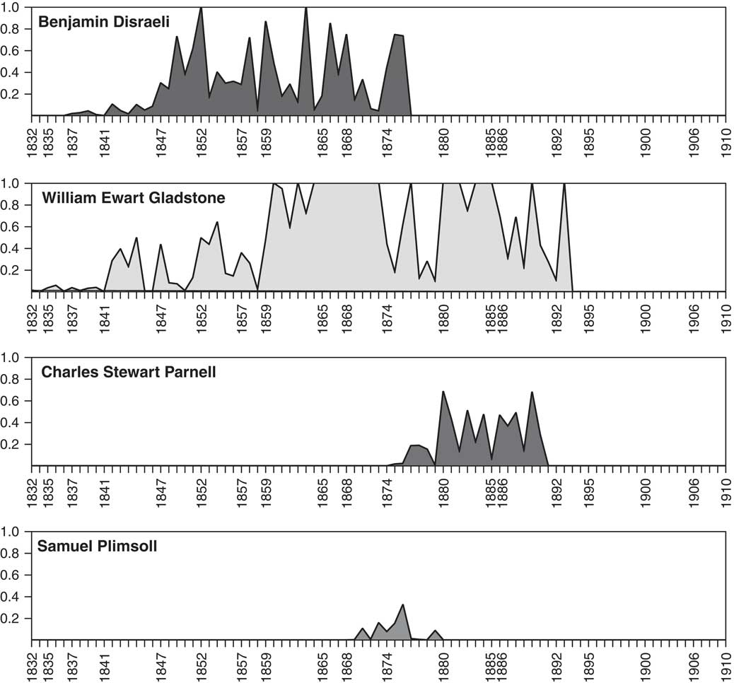
Fig. 5 Burstiness profile of MPs over time. Note: the y-axis of the plots is the ‘standardized’ burstiness of the term, a rescaled metric where a value of 1 corresponds to the most bursty MP that session, while a value of 0 refers to the least bursty MP. The x-axis labels correspond to the beginnings of the various parliaments during the period.
Alternative Measures: ‘Speechiness’
One concern readers may have is that burstiness is simply a stand-in (that is, a proxy) for ‘speechiness’: that is, our metric measures nothing more than the varying ability or willingness of MPs to make speeches. This is not the case: the correlation between the burstiness of opposition MPs and the number of speeches they make varies between 0.19 (1892) and 0.90 (1847) over the sessions as a whole, with a mean of 0.63. These variables are not measuring the same thing: while it is true that an MP may be non-bursty because he makes no speeches, making lots of speeches is no guarantee of being bursty. In particular, an MP who makes (perhaps thousands of) speeches that are simple responses, or contain terms that are not picked up by others, will not be bursty.Footnote 74
More philosophically, another reason to eschew speechiness as a measure is that it over-rewards procedural responsibility and opportunity relative to actual agenda-setting ability. To see this, consider the speakers of the House of Commons. With power over recognition and organization of debates in the chamber, speakers make many speeches. Yet since they are non-partisan figures without incentives or opportunities to introduce or discuss policy proposals, we would not expect them to be more bursty than leaders of the government and opposition.Footnote 75 To see the problems that insufficient attention to such a distinction can produce, consider Figure 6, which compares the speechiness and burstiness of the seven speakers in our data, in chronological order. On the y-axis we report the quantile position of the speaker’s mean scores – in terms of the number of speeches he made, and his burstiness – relative to all other MPs serving in the same sessions who made at least one speech. We see immediately (top line and points) that every speaker is close to the maximum of the empirical cumulative distribution function (CDF) in terms of speeches, occupying somewhere around the 97th percentile on this measure. By contrast, the burstiness metric (bottom line and points) has the speaker rightfully downplayed in terms of score – around the 80th percentile, on average. Clearly then, relative to speechiness, burstiness avoids directly reproducing procedural power in favor of a more genuine measure of policy agenda setting. It is thus a better measurement strategy for our current work, especially for opposition members who have few de jure powers.

Fig. 6 Speakers: number of speeches (speechiness) vs. burstiness scores. Note: the x-axis names the speakers in chronological order. The y-axis is the position in the CDF of all speeches and burstinesss scores (among those MPs who made a speech) of the (mean) speakers’ speechiness and burstiness for the sessions in which he served.
Before moving to our results, we underline an assumption that is obviously present in our work: that, in fact, the existence of the Shadow Cabinet can be discerned from an inspection of speech records in the House of Commons. One concern might be that perhaps, prior to more widespread democratization, the Shadow Cabinet made its presence felt in other ways – for example, via electioneering in the constituencies. We acknowledge this, but would claim that at the very least, our study is of the Shadow Cabinet in a sense similar to that as in the modern period – that is, as a legislative force.
RESULTS
We have established a metric for measuring MPs’ individual agenda-setting abilities. Ultimately, we want to use it to explore the ways in which the informal institution of interest – that is, that Shadow Cabinet members become Cabinet members – evolved over time. This requires three interrelated steps. First, we need to show how and when the opposition as a whole organized, and collectively paid more attention to agenda control. Secondly, within that opposition, we need to explore how agenda-setting power became concentrated in a leadership group. That is, we need to assess whether and when a Shadow Cabinet could have been said to emerge. Thirdly, given that we have established that the opposition organized, and that they did so under a Shadow Cabinet, we need to show that the latter became ministers at the exchange of power and that this relationship was non-constant over time.
Opposition Burstiness Over Time
We begin by considering the agenda-setting ability of the opposition, and how this changes over time. Of course, our metric above is absolute: it calculates a raw number pertaining to individuals, or groups of individuals, and their ability to raise issues that draw attention in Parliament. In practice, this means that burstiness may be generally higher under two conditions: (1) when (exogenously) there are more things to be bursty about – for example, a war, famine or some other event of note occurs or (2) when there are more opportunities to talk, since this lengthens the period (in speech terms) when bursts may appear. Given these facts, we consider the burstiness of the opposition relative to the Cabinet. In particular, we begin this section by taking the ratio of mean opposition burstiness to mean Cabinet burstiness for every session in our data.
In the upper panel of Figure 7 we plot that quantity: it appears as the jagged line that peaks and troughs, moving left to right, reaching its zenith around 1857 (when the Cabinet was about 40 times more bursty), and its nadir around 1885 (when the Cabinet was about 5 times more bursty). Note that for clarity, we demarcate the x-axis using general election dates for the period.
Fig. 7 Ratio of (mean) burstiness: cabinet to opposition, cabinet to (government party) backbenchers. Note: one change point was found in the opposition ratio time series, marked on the plot with the broken line and the mean of ratio given on the either side.
The first observation from the upper panel of Figure 7 is that the Cabinet was always more bursty than the opposition, on average: notice that the line is never below 1. Given the dominance of the Cabinet over procedure from the 1830s onwards, this is not per se surprising: ministers have more opportunities to be bursty, and presumably by the very nature of their jobs have more ready access to information that can become bursty (for example, reports of officials figures or policies). However, moving left to right, we see a generally decreasing ratio: the smooth lowess line makes the point very clear. Put otherwise, the opposition becomes more than the Cabinet, with the key change apparently happening between about 1870 and 1885. To place this result on a more sound statistical footing, we conducted structural break tests (in the sense of Bai and Perron).Footnote 76 We found one break in the ratio data, dating to the third session of the parliament beginning after the 1880 general election: in the figure, we present this point as a broken line and note that the mean ratio dropped by over 50 per cent, from 16.91 to 7.25 after the change point. Though we will give a more detailed analysis below, note that this aggregate realignment of agenda-setting power is commensurate with our claim that a set of opposition leaders – that is, a Shadow Cabinet – is emerging and making its influence known after suffrage extension.
An obvious concern on seeing such a result is that there is nothing ‘special’ about the opposition: perhaps the Cabinet’s agenda-setting ability was in secular decline from the 1870s onwards? We can go some way toward refuting this suggestion by studying the lower panel of Figure 7, where we consider the (mean) ratio of the Cabinet to government backbenchers. Notice that both the underlying ratio and the smoothed lowess are essentially constant. We find no breakpoints here using the usual formal tests. Ultimately then, we can conclude that the change in the ratio for the opposition is specific to that side of the House of Commons, and not a general artifact of changing Cabinet roles or priorities at the time.
Opposition Outliers as a ‘Front Bench’
Having established that the opposition was increasingly aggressive in its agenda setting just after the Second Reform Act, we next seek the precise mechanics of that change. That is, we wish to understand exactly how the opposition asserted its control. Recall that one possibility is that it increasingly mimicked the government party’s authority structure by establishing an ‘executive’ core of frontbenchers to set policy and rebuff the cabinet, with a pliant majority of opposition backbenchers formed up behind them. In Figure 8 we examine the evidence for such a claim.

Fig. 8 Concentration of agenda-setting power in the opposition over time. Note: the top panel shows the changing distribution of burstiness for the opposition; the middle panel shows the changing median and 90th percentile but using standardized data, by session; the lower panel shows the (declining) number of outliers over time – consistent with the emergence of a ‘Shadow Cabinet’.
In the upper portion of Figure 8, we report boxplots of the burstiness of opposition parties (specifically, the Conservatives and Liberals) over time. The points (circles and squares) denote outliers, defined in the usual way as points above (and below) 1.5 times the interquartile range of the given session. Note immediately that, in practice, all outliers are in the right tails of their distributions: that is, the median opposition member has a very low burstiness for the entire period (and, indeed, it is close to 0 on this measure). Secondly, we see a surge in the magnitude of the outliers around 1880: indeed, some of the largest burstiness scores are recorded between 1880 and 1892. Formal time-series tests on the means of each session show that there is one break point, demarcated by a broken line during the third session of the parliament meeting in 1880. The standard deviation of the burstiness yields an almost identical finding, although the change point corresponds to the second session of 1880. Finally, we report the changing means and standard deviations themselves: prior to the break, we have a mean of 211,688.28, while the standard deviation is around 7 million. By contrast, the latter part of the time series has a mean and standard deviation an order of magnitude higher. We conclude that the ‘average’ burstiness of the opposition was increasing, while simultaneously showing more variance. Given that the floor value of the metric is zero, the implication of the top panel is that some individuals are increasingly pulling away from average members.
To make this point clearer, consider the middle panel, where we have standardized the measure by session, meaning all MPs fall between 0 and a burstiness of 1. There, the flat dashes at the bottom of the figure are the medians, while the points are the positions of the 90th percentile members of the opposition (which typically represents an MP ranked around the 20th most bursty in his party). The solid line represents a lowess-smoothed curve through those points, and it can be readily seen that its slope increases in magnitude around the time of the Second Reform Act. Notice that while there is some noise, the slope is clearly upwards, and by the turn of the century the 90th percentile has pulled away from the medians (on average) substantially.
To test our intuitions more precisely, the bottom panel of Figure 8 reports the number of opposition outliers over time. Clearly, there is a downward trend: beginning with around 70 outliers, the opposition has around 50 outliers by the 1870s, and fewer than 20 by the end of the period. Again, we use a formal structural break test which in this case revealed two breaks: one in the last session of the 1865 parliament, and the second in the first session of the parliament meeting after the 1886 election. In both cases, the mean is reduced. Importantly for our purposes, the average number of outliers is reduced to the approximate size – below 20 – that we would expect for a Shadow Cabinet of spokesmen on various issues of governance. To reiterate: here we find that the date of the Second Reform Act (1867) was a crucial transition point for the emergence of a small(er) set of bursty individuals on the opposition benches, congruent with the existence of a cadre of senior MPs in leadership roles.
On seeing these plots, readers may be skeptical about our claims regarding the importance of the Second Reform Act, given that subsequent sessions – for example, 1880 and 1902 in the top panel, and the mid-1880s in the bottom panel – are also associated with surges and changes to the opposition’s relative burstiness.Footnote 77 Two comments are in order: first and foremost, these dates obviously occur after the Second Reform Act and are thus consistent with notions that 1867 was crucial to altering the data-generating process in a large and general way. Secondly, we would reiterate our comments about the cautious interpretation of timing: the claim is not of a binary ‘switch’ in behavior (and thus an outright repudiation of any other plausible causal agent), but rather a continuous change process that receives a fillip after suffrage expansion.
Burstiness and Future Cabinet Status
One way to verify our presumption – that the outliers from Figure 8 are a ‘Cabinet in waiting’ – is to show that, in fact, they went on to fill Cabinet roles when their party found itself next in government. To examine this possibility, we considered the 14 times that power switched, in the sense that a new party previously in opposition now formed the government, during the period. For the opposition members in each switching session, we pooled the data and regressed their (binary) status as a Cabinet member in the next session on their (binary) status as an outlier in the previous period, along with a time indicator, and burstiness as a robustness check. Because we have some repeated observations of MPs, we cluster standard errors at the MP level. We make no claims that this causally identifies the effect of Shadow Cabinet membership on subsequent office holding: even if outlier status were a perfect measure of Shadow Cabinet membership, members of the Shadow Cabinet undoubtedly differ from other MPs in many ways that would be important to prospects for promotion. However, such an analysis can establish whether the evidence is broadly consistent with our claims.
The relevant part of our results can be seen in Table 2. In Model 1, we use outlier status and ‘session number’ since the Great Reform Act – literally, the number of sessions of parliament that have occurred since 1832 (thus the first session in our data is given the value 1, the second is 2 and so on). We see a positive association for both variables: that is, being an outlier helps an MP be promoted the next time his party is in office, and, in fact, as time passes he is unconditionally more likely to be promoted. This latter finding is sensible, because ministers were increasingly drawn from the Commons rather than the Lords. In Model 2, we try an alternate measure of ‘leadership-ness’ – the number of speeches given by the MP. As we see from the higher Akaike information criterion (AIC), this model does not fit the data as well as the previous one, which implies that using the burstiness outlier metric provides useful extra leverage over more traditional alternatives.
Table 2 Coefficients for Logistic Regression of Cabinet Membership on Outlier Status, Burstiness, Years Since Great Reform Act and Interaction Terms

Note: standard errors clustered on MP. Significant at †p<0.10, *p<0.05, **p<0.01; ***p<0.001.
In Model 3 we add our key interaction term between time and outlier status. As expected and consistent with our claims, the coefficient on being an outlier remains positive and significant. The coefficient on session number is similarly positive and significant, and is larger in this specification. Importantly, the interaction effect is significant, and smaller than the combined effect of being an outlier and the session number.Footnote 78 Thus the net effect of being an outlier is that one was more likely to be promoted to office as time passed.Footnote 79 Notice that this model has a smaller AIC than the previous effort, suggesting it is a better fit to the data. Moreover, a likelihood ratio test favors the model with the interaction. Finally, in Model 4, we add a variable measuring whether or not (1 or 0) the member had previously served in the Cabinet. As expected, the coefficient is positive, but – crucially – being an outlier still matters (our coefficient is statistically significant). All told, our burstiness outlier metric is sound and helpful: it genuinely measures some notion of being in the Shadow Cabinet that is not simply captured by the number of speeches given, or having been previously selected as a Cabinet minister.Footnote 80
The fact that the probability of advancing to Cabinet as a product of being a bursty outlier increases as time goes on does not per se rule out either theory as a possibility. But nor do we intend it to alone. Rather, we consider it part of a series of evidential pieces that add up to a story in which something other than the immediate aftermath of the Great Reform Act matters: there is no plateau here, and with every passing session the relationship between burstiness and Cabinet office becomes stronger. This serves in part to imply that we have successfully identified a good measure of Shadow Cabinet membership.Footnote 81
Summary
We have three interrelated results:
-
1. Though the Cabinet was always more bursty than the opposition, the latter became relatively more assertive in agenda-control terms around the time of the Second Reform Act (1867).
-
2. Within the opposition, outliers (extremely bursty individuals) became fewer in number over time, with marked shifts downwards at the time of the Second Reform Act, and in the mid-1880s. By the turn of the twentieth century, a group of individuals approximately the size of a Shadow Cabinet had emerged.
-
3. The key informal institution of interest – the purported relationship between being in the Shadow Cabinet and being in the Cabinet when the party in question took power – was present for the entire period, and became increasingly strong over time (an outlier in later sessions was more likely to be promoted to Cabinet office than an outlier in earlier sessions).
DISCUSSION
Informal institutions form the core of practical politics in Westminster systems, where statute law is often silent: this includes the role of parties (there is none, constitutionally speaking), the role of whipping (never officially acknowledged) and the role of the prime minister (which has never been formally defined). This means that scholars of these polities, and comparative politics more generally, have a particularly pressing interest in understanding how inferences may be made about these norms and rules, if they are to plot their emergence and evolution over time. In this article, we considered the role of the Shadow Cabinet as a government in waiting, a vital organization that ensures citizens an alternative to the present government at election time – even if this does not ultimately mean that the people’s will is implemented as policy.Footnote 82
We showed that informal institutions are helpfully modeled using latent variables. Our solution here was to apply new text-as-data methods to almost a million speeches by MPs between the First and Fourth Reform Acts. Using a burstiness metric, we showed that after the 1870s, an increasingly small group of opposition leaders closed the gap in terms of agenda setting in their partisan competition with the Cabinet. Intriguingly, though the Cabinet began its characteristic dominance of procedure in the 1830s,Footnote 83 it appears that it was the broadening of suffrage that accelerated the emergence of the Shadow Cabinet as an institutional force. Our work joins a large literature on the effects of suffrage expansion on political behavior and policy making at Westminster,Footnote 84 and by moving the focus to the opposition it also contributes to the study of comparative parliamentary politics.Footnote 85
Our work has several broader implications. First, we demonstrated an important case in which an (informal) institution arose organically as a counterpoint to a pre-existing organization – the Cabinet – when an external stimulus was presented (in our case, a party-orientated electorate). Our work thus joins a literature that deals with institutionalism,Footnote 86 and the specific mechanisms by which institutions evolve.Footnote 87 Again, we think our measurement strategy is a way to proceed when faced with the task of charting the development of such organizations over time. Secondly, we took an explicitly agenda-setting approach – a topic of very general interest to political scientists.Footnote 88 Typically, measuring the extent to which bodies or individuals have the power to set the agenda is difficult – especially in parliamentary systems where, in day-to-day operations, oppositions lose and governments win. We have partially resolved that issue.
This article raises several interesting questions that we have left unanswered. First, we have not looked at the screening and selection mechanisms by which MPs joined the Shadow Cabinet; a specific career path focus for the Victorian period, in line with more modern work,Footnote 89 is called for. Secondly, our technique allows for helpful (weighted) word-based summaries of debates. Our focus here was on the relative burstiness of sets of individuals, but it would presumably be beneficial to those interested in ideological changes in Westminster legislatures over timeFootnote 90 to use a metric like ours to get a sense of exactly how – that is, on what issues – MPs became divided or unified as their parties evolved. Related to this endeavor, integrating burstiness with debate sequencing – that is, who speaks after whom and what it signals about strengthening informal relationships across the floor over time – is a task worthy of attention. Thirdly, while it is well known that democratization in Britain included moves away from staffing top party and governance roles with members of the House of Lords, unfortunately we did not have peers’ speech records available for similar analysis to that above. It would certainly be intriguing to document any potential shifting burstiness from one chamber to another over time, especially if such changes affected how government and opposition interacted in both places. Finally, with the speech records of other legislatures – such as the US CongressFootnote 91 – increasingly available online, it would be intriguing to analyze the burstiness of terms in a comparative context, to see how different systems converge or diverge in term use over time. We leave such efforts for future work.


