2.1. ADS-B data transmission

ADS-B data is broadcast by an ADS-B OUT unit, which periodically broadcasts its state vector (position and velocity), as well as other information derived from on board systems, in a format suitable for ADS-B IN-capable receivers. The ground station collects this data from all aircraft in the airspace, processes the data in the Air Traffic Control (ATC) system, and broadcasts the data back to the airspace. An aircraft receives this data through ADS-B IN (FAA, 2010). The ADS-B system architecture is schematically illustrated in Figure 1 (Strohmeier et al., Reference Strohmeier, Schafer, Lenders and Martinovic2014).

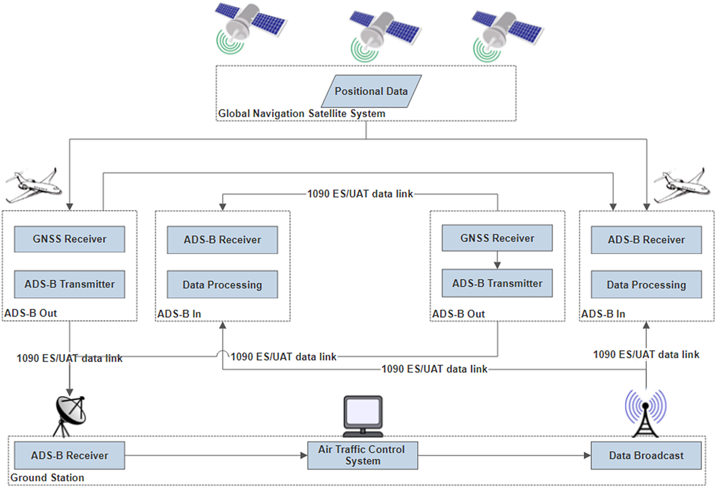
Figure 1. ADS-B data link in air traffic management (Strohmeier et al., Reference Strohmeier, Schafer, Lenders and Martinovic2014).

2.2. ADS-B positioning uncertainty quantification

The broadcast position information is derived by the on board satellite navigation receiver. Due to errors in signal transmission, noise in satellites and receivers, and possible satellite faults, the position information provided by the GNSS receiver has its own uncertainty that is required to be measured and broadcast. Two types of uncertainty are provided: the Estimated Position Uncertainty (EPU) and the integrity containment Radius (R_c). These types of uncertainty are calculated based on two performance parameters of satellite navigation: accuracy and integrity. The EPU refers to the 95% confidence bounds of positioning error in the horizontal direction with no satellite fault, which is classified by Navigation Accuracy Category for Position (NACp). NACp is reported so that surveillance applications may determine whether the reported position has an acceptable level of accuracy for the intended use. The R_c is the 99.99999% confidence level of positioning uncertainty considering satellite faults, which is represented by the Navigation Integrity Category (NIC). The FAA specifies the acceptable values of NACp and NIC in ADS-B data as presented in Table 1 (RTCA, 2006).

Table 1. ADS-B Position Information accuracy and integrity classification (RTCA, 2006)

2.3. Existing separation analysis using ADS-B

The current separation standards are based on the provisions of International Civil Aviation Organization (ICAO) document “Doc 4444” (ICAO, 2016), which specifies minimum vertical separation for Instrument Flight Rules (IFR) flight as 1000 ft (300 m) below Flight Level (FL) 290 and 2,000 ft (600 m) above FL290. It also specifies five nautical miles in the horizontal direction as the minimum separation when surveillance systems (for example, based on radar, ADS-B, or Multi-Lateration (MLAT)) are used in en-route airspace, while three nautical miles is specified for terminal airspace at lower altitudes. Several studies focus on the separation analysis using ADS-B based surveillance systems in NextGen (Gazit and Powell, Reference Gazit and Powell1996; Powell et al., Reference Powell, Jennings and Holforty2005). The focus is on the increased capacity of the airspace system using ADS-B. Other studies focus on the safety and risk analysis associated with the changing of aircraft separation criteria (Shepherd et al., Reference Shepherd, Cassell, Thapa, Lee, Shepherd, Cassell, Thapa and Lee1997; Everdij et al., Reference Everdij, Blom and Bakker2007; Herencia-Zapana et al., Reference Herencia-Zapana, Jeannin and Munoz2010). The MITRE Corporation investigated ADS-B surveillance separation error and performed sensitivity analysis (Jones, Reference Jones2009).

Most existing studies have investigated the uncertainty quantification of individual units (or aircraft) and its impact on the risk assessment. In classical statistics and probability theory, this refers to the Uncertainty Quantification (UQ) of a single random variable. The mean and variance parameters and Probability Density Function (PDF) are generally used for this purpose. In the general context of Air Traffic Management (ATM), most concerns are for the separation of aircraft (for example, avoiding mid-air collisions or runway incursions). Thus, two or more aircraft will be involved in the safety metrics for ATM. If the uncertainties are considered, this belongs to the uncertainty quantification of multiple random variables. From a statistical point of view, the safety concern of ATM (that is, the probability of failure) is usually related to the tail behaviour of the probability density function. This is because most systems are designed to be safe and failure has a very small probability (that is, the tail region). The correlation effect will change the variance estimation and tail shape significantly. Thus, development of a model to systematically investigate the correlation effect will be very valuable for future operation and decision making in ATM. Therefore, the motivation of this study is to close this gap by providing a rigorous model to investigate the mean and correlation effect of two or more aircraft in their separation loss probability evaluation. To limit the discussion, this study focuses on a pair of aircraft, but the methodology is generic and can be extended to multiple aircraft.

3.1. Position error

The following equation is the basic observation equation for satellite navigation in normal conditions:

(1)$${\bf z}={{\bf Hx}}+{{\bf v}}+{{\bf f}} $$

where z is the measurement vector whose elements are pseudoranges from viewable satellites to the receiver, H denotes the observation matrix, v is a vector composed of zero mean, unit-variance independent and identically distributed (iid) random variables and f represents the abnormal bias in pseudoranges that is caused by a satellite fault. Each element of v represents various normal errors, including satellite ephemeris and clock error, ionospheric delay, tropospheric delay, multipath noise and receiver noise. All these errors are assumed to follow independent Gaussian distributions. The element in f corresponding to a faulty satellite is non-zero. In fault-free condition, f = 0.

The estimated position is expressed as a least square solution of Equation (1) as:

(2)$$\hat{{\bf x}}={{\bf H}}^{{{\ast }}}{\bf z} $$

where:

(3)$${{\bf H}}^\ast =\lpar {{{\bf H}}^{{\bf T}}{{\bf H}}} \rpar ^{-1}{{\bf H}}^{{\bf T}} $$

Substituting Equation (1) into Equation (2), the following equation is obtained:

(4)$$\hat{{\bf x}}={{\bf H}}^{{{\ast }}}\lpar {{\bf Hx}}+{\bf v}+{\bf f}\rpar ={\bf x}+{{\bf H}}^{{{\ast}}}\lpar {\bf v}+{\bf f}\rpar $$

where x denotes the real state vector including Three-Dimensional (3D) position and clock bias. The estimated position error is expressed as:

(5)$${{\bi \varepsilon}}=\hat{{\bf x}}-{{\bf x}}={{\bf H}}^{{{\ast }}}{{\lpar {\bf v}+{\bf f}\rpar }} $$

For two nearby aircraft (here, aircraft A and aircraft B), their surveillance separation is expressed as:

(6)$$\eqalign{\hat{{\bf s}}_{{{{\bf A}\comma {\bf B}}}} & =\hat{{\bf x}}_{{{\bf A}}}-\hat{{\bf x}}_{{{\bf B}}} \cr &=\hat{{\bf x}}_{{{\bf A}}}-{{\bf x}}_{{{\bf A}}}-\lpar \hat{{\bf x}}_{{{\bf B}}}-{{\bf x}}_{{{\bf B}}}\rpar +\lpar {{\bf x}}_{{{\bf A}}}-{{\bf x}}_{{{\bf B}}}\rpar \cr &={{\bi \varepsilon }}_{{{\bf A}}}-{{\bi \varepsilon }}_{{{\bf B}}}+{{\bf s}}_{{{{\bf A}\comma {\bf B}}}}} $$

where $\hat{{\bf x}}_{{{\bf A}}}$ and $\hat{{\bf x}}_{{{\bf B}}}$ represent the positions provided by the receivers on aircraft A and aircraft B, respectively. ε_A and ε_B denote the position errors of aircraft A and aircraft B, respectively. s_A,B represents the real separation between A and B.

Equation (6) can be expressed as:

(7)$${{\bi \varepsilon }}_{{{\bf s}}_{{{\bf A}}\comma {{\bf B}}} } ={{\bi \varepsilon }}_{{\bf A}} -{{\bi \varepsilon }}_{{\bf B}} $$

where ${{\bi \varepsilon}}_{{{\bf s}}_{{{\bf A}}\comma {{\bf B}}}}$ denotes the separation error between A and B, which is formulated as:

(8)$${{\bi \varepsilon }}_{{{\bf s}}_{{{\bf A}}\comma {{\bf B}}}} =\hat{{\bf s}}_{{{{\bf A}\comma {\bf B}}}}-{{\bf s}}_{{{{\bf A}\comma {\bf B}}}} $$

Substituting Equation (5) into Equation (7), the following separation error model can be obtained:

(9)$${{\bi \varepsilon }}_{{{\bf s}}_{{{\bf A}}\comma {{\bf B}}} } ={{\bf H}}_{{\bf A}}^\ast \lpar {{{\bf v}}_{{\bf A}} +{{\bf f}}_{{\bf A}} } \rpar -{{\bf H}}_{{\bf B}}^\ast \lpar {{{\bf v}}_{{\bf B}} +{{\bf f}}_{{\bf B}} } \rpar $$

For receivers on two nearby aircraft, the satellite ephemeris and clock errors are assumed to be identical at the same time. The errors in transmitting path, including ionospheric delay, tropospheric delay and multipath noise are not identical, but are highly correlated. The receiver noise of different receivers are assumed to be independent. In the condition that the two nearby aircraft use the same satellite set to navigate, the observation matrices H_A and H_B are almost equal. In addition, the fault vector f_A equals f_B when the two aircraft see the same satellite sets. Thus, qualitative analysis shows that ε_A and ε_B should be highly correlated when they are close to each other and see the same satellite. The same conclusion cannot be directly extended to the case when aircraft see different satellite sets. One possible scenario for large separation error from Equation (9) is when both H_A, f_A and H_B, f_B are large. Details are explained below.

It should be noted that even two nearby aircraft could use different satellite sets to navigate because of the following reasons:

• • Users set different mask angles. Document “FAA AC 90-114A” (FAA, 2010) allows an operator to select a proper mask angle;

• • Aircraft use different navigation constellations, for example, one aircraft uses GPS while the other uses a joint GPS and Galileo constellation;

• • Signal loss due to ionospheric scintillation or mountain blocking;

• • A satellite just emerges in the view of one aircraft but not in the other.

In this condition, the difference between H_A and H_B can be large. This is one contributor to the large separation error in the proposed model (Equation (9)). Another contributor for the large separation error is satellite faults. A GPS satellite fault is an event with a relatively frequent occurrence. The GPS Standard Positioning Service (SPS) Performance Standard (US DoD, 2001) provides a major service failure rate of three times per year lasting no longer than six hours. This rate can be converted to a fault probability of 10⁻⁵ for each GPS satellite. In the condition that the two aircraft use the same satellite set to navigate, a satellite fault will not influence the separation error as the faults are cancelled in the separation error calculation.

In practice, one aircraft cannot know what satellite set the other aircraft (intruder) is using and the GNSS receiver must carry out fault detection to mitigate the impact. A fault can be detected by hypothesis tests. A fault occurring in the i-th satellite is one of the hypotheses, being denoted as H_i. When setting the i-th satellite corresponding row to zero, the observation matrix becomes:

(10)$${{\bf H}}_{{0}{{\bf i}}} =\lpar {{{\bf I}}-{{\bf A}}_{{\bf i}} {{\bf A}}_{{\bf i}}^{{\bf T}} } \rpar {{\bf H}}^{{\bf T}} $$

where A_i is a n × n _i matrix with ${\bi I}_{{\bi n}_{i}}$ occupying the first n_i rows and columns. Other elements of A_i are zero. Thus:

(11)$${{\bf A}}_{{\bf i}} =\lsqb {{\bf I}}_{{{\bf n}}_{{\bf i}}}\ 0_{{\bf n}_{{\bf i}}\times \lpar {{\bf n}}-{{\bf n}}_{{\bf i}}\rpar }\rsqb ^{{\bf T}} $$

The position estimation without the i-th satellite is expressed as:

(12)$$\hat{{\bf x}}_{{{\bf i}}}={{\bf H}}_{0{{\bf i}}}^{{{\ast }}}{\bf z} $$

where:

(13)$${{\bf H}}_{0{{\bf i}}}^\ast =\lpar {{{\bf H}}_{0{{\bf i}}}^{{\bf T}} {{\bf H}}_{{0}{{\bf i}}} } \rpar ^{-1}{{\bf H}}_{{0}{{\bf i}}}^{{\bf T}} $$

The difference of the positions with and without a satellite fault is expressed as:

(14)$${{\bi \Delta }}\hat{{\bf x}}_{{{\bf i}}}=\hat{{\bf x}}_{{{0}}}-\hat{{\bf x}}_{{{\bf i}}}=\lpar {{\bf H}}^{{{\ast}}}-{{\bf H}}_{0{{\bf i}}}^{\ast}\rpar {\bf z} $$

where $\hat{{\bi x}}_{{\bf 0}}$ denotes the position solution determined by using the full-set satellite. Extracting the interested state of ${\bi \Delta} {\hat{\bi x}}_{\bf i}$, for example, a state in an axis direction of a coordinate used to formulate the observed matrix H is:

(15)$${\rm x}_{{\rm ss\comma i}}={{\bf e}}_{{{\bf d}}}^{{{\bf T}}}{{\bi \Delta }}\hat{{\bf x}}_{{{\bf i}}} $$

where d = 1, 2, 3 denotes three dimensions of position, ${\bi e}_{{\bi d}}^{{\bi T}}$ denotes a m × 1 vector whose d-th element is one and whose other elements are zeros.

In normal condition, x_ss,i follows a Gaussian distribution (Pervan et al., Reference Pervan, Pullen and Christie1998):

(16)$$\hbox{x}_{{\rm ss}\comma {\rm i}} \sim \hbox{N}\lpar {0\comma \; \sigma_{ss\comma i}^2 } \rpar $$

where σ _{ss, i} denotes the standard deviation and can be calculated as (Joerger et al., Reference Joerger, Chan and Pervan2014):

(17)$${\sigma }_{{\rm ss}\comma {\rm i}}^2 ={{\bf e}}_{{\bf d}}^{{\bf T}} \lpar {\lpar {{{\bf H}}_{0{{\bf i}}}^{{\bf T}} {{\bf H}}_{0{{\bf i}}} } \rpar^{-1}-\lpar {{{\bf H}}^{{\bf T}}{{\bf H}}} \rpar^{-1}} \rpar {{\bf e}}_{{\bf d}} $$

The threshold for fault detection is expressed as (Blanch et al., Reference Blanch, Walter, Enge, Lee, Pervan, Rippl and Spletter2012):

(18)$$\hbox{T}_{{\rm ss}\comma {\rm i}} =\hbox{K}_{{\rm fa}\comma {\rm i}}{\sigma }_{{\rm ss}\comma {\rm i}} $$

where

(19)$$\hbox{K}_{{\rm fa}\comma {\rm i}} =\hbox{Q}^{-1}\left({\displaystyle{{\hbox{P}_{{\rm fa}\comma {\rm i}} }\over{2}}} \right)$$

and Q is the cumulative distribution function of a standard Gaussian distribution. P _{fa, i} is the continuity budget (false alarm probability) allocated to the i-th fault hypothesis.

3.2. Separation loss probability evaluation

The above discussion focuses on the uncertainty quantification in a probabilistic position error model. This section focuses on the estimation of separation loss probability using these quantified uncertainties. The FAA specifies the safe separation requirement. For example, the five nautical miles rule is applied laterally in en-route environments. Risk occurs when the positioning system indicates the requirement is satisfied and the actual separation is not. In this study, we define a separation loss probability to quantify this risk level. The separation loss probability is defined as a conditional probability that the real separation of an aircraft pair is smaller than the safe separation but the surveillance separation (based on ADS-B information) is greater than the safety rule without an alert. The separation loss probability is formulated as:

(20)$$\hbox{P}_{{\rm sr}\comma {\rm i}} =\hbox{P}\lpar {\rm s}< \hbox{D}\comma \; \hbox{q}< \hbox{th}\vert \hat{{\rm s}}>{\rm D}\comma \; {\rm H}_i\rpar $$

where s is the real separation between the two aircraft, D is the safe separation specified by the FAA in the corresponding flight phase, q is the fault detection test statistic (q equals to x _{ss, i} using solution separation method (Pervan et al., Reference Pervan, Pullen and Christie1998)), ${\hat s}$ is the surveillance separation based on ADS-B data, H _i(i = 0, 1, …, n) is the fault hypothesis as discussed in the last section and H ₀ denotes the hypothesis of no fault occurring. Because the probability of simultaneous fault of multiple satellites is very small, we just consider the single fault case in this paper. The total separation loss probability is bounded by the following inequation:

(21)$$\hbox{P}_{{\rm sr}} \le \mathop \sum \limits_{{\rm i}=0}^{\rm n} \hbox{P}_{{\rm sr}\comma {\rm i}} \hbox{P}\lpar {\hbox{H}_{\rm i} } \rpar +\hbox{P}_{{\rm not}\_{\rm monitored}} $$

where P(H _i ) is the probability of hypothesis H _i.

The terms of real separation and surveillance separation in Equation (20) have the following relationship:

(22)$$\hbox{s}=\hat{{\rm s}}-\varepsilon $$

where ε denotes the separation error. The GPS position error follows a Gaussian distribution for every single aircraft if the independent identical distribution (iid) noise is assumed in measurements. The separation error equals the difference of position errors of aircraft A and aircraft B:

(23)$$\varepsilon =\varepsilon_{A0} -\varepsilon_{B0} $$

An aircraft (aircraft A) receives the position information of the other (aircraft B) aircraft through the ADS-B IN system, including NACp (EPU) and NIC (R_c). NACp (EPU) indicates the accuracy of the other aircraft's position at the 95% confidence level in the fault-free assumption. NIC (R_c) represents the integrity information of positioning, which is the protection level to quantify the much higher level (for example, 1–10⁻⁷) positioning uncertainty considering the fault condition. In other words, this high-level uncertainty (that is, integrity risk probability), denoted as P_int, refers to the probability of the true position exceeding the protection level. We use the following conservative assumption:

(24)$$\varepsilon_{B0} \sim N\left(-\hbox{Rc}_{\rm B}\comma \; \left({\displaystyle{{{\rm EP}{\rm U}_{\rm B}} \over 2}} \right)^2\right)$$

The probability of the condition that is worse than the above assumption is 0 · 5P_int. The other conservative assumption is made that the measurement noises of the two aircraft are statistically independent. Then the separation error is:

(25)$$\varepsilon \sim N\left({\hbox{g}\lpar {{\bf f}} \rpar +\hbox{Rc}_{\rm B} \comma \; \sigma_0^2 +\left({\displaystyle{{\hbox{EPU}_{{\rm B}} }\over{2}}} \right)^2} \right)$$

where g(f) represents a function of the fault vector f, σ ₀ denotes the position error standard deviation of aircraft A, and EPU_B is the accuracy parameter of aircraft B received by aircraft A. For aircraft A, when it receives the ADS-B data, the real-time separation loss probability is bounded as the following expression:

(26)$$\hbox{P}_{{\rm sr}\comma {{\rm A}}} \le \mathop \sum \limits_{{\rm i}=0}^{{\rm n}} \max_{f_i } P\lpar \varepsilon>\hat{{\rm s}}-{\rm D}\comma \; {\rm q}< {\rm th}\vert \hat{{\rm s}}>D\comma \; {\rm H}_{{\rm i}}\rpar P\lpar {\rm H}_{{\rm i}}\rpar +P_{not\_monitored}+0{\cdot} 5P_{{\rm int}} $$

The above bound can be obtained using a search method to find the fault vector f that maximises the right term of the above inequation. In order to reduce the computational complexity, we further simplify it as follows:

(27)$$\eqalign{\varepsilon -q &=\varepsilon _{A0} -q-\varepsilon _{B0} \cr &=\varepsilon _{A0} -x_{i\comma ss} -\varepsilon _{B0} \cr &=\varepsilon _i -\varepsilon _{B0}} $$

where the ε _i denotes the error of $\hat{x}_i$ expressed in Equation (12). Then we have a transformation for the first inequation:

(28)$$\varepsilon_i -\varepsilon _{B0} >\hat{s}-D-th $$

In the fault hypothesis, H _i, and under the assumption of independent measurement noise of both the aircraft, the term ε _i − ε _B0 is denoted as ε _s in the following distribution:

(29)$$\varepsilon _s \sim N\left({\hbox{Rc}_{\rm B} \comma \; \sigma_i^2 +\left({\displaystyle{{EPU_B} \over 2}} \right)^2} \right)$$

where $\sigma _{i}^{2} $ represents the variance of $\hat{x}_i$. The upper bound of the separation loss probability can be expressed as:

(30)$$P_{sr\comma A} \le \mathop \sum \limits_{{\rm i}=0}^{{\rm n}} P\lpar \varepsilon_s >\hat{s}-D-th\vert \hat{{\rm s}}>D\comma \; {\rm H}_{\rm i}\rpar P\lpar {\rm H}_{\rm i}\rpar +P_{not\_monitored}+0{\cdot} 5P_{int} $$

The above upper bound is computationally efficient and is conservative for separation loss probability evaluation.

Other metrics might be more convenient for practical use, such as the protection distance, pd:

(31)$$\hbox{pd}=\hat{s}-{\rm D} $$

The protection distance can be calculated by solving Equation (30) if the separation loss probability is known. The protection is defined so that a pilot will be aware of how much extra distance is needed to keep a low separation loss probability. Figure 2 illustrates the relationship between separation requirement, protection distance and surveillance separation.

Figure 2. Illustration of relationship among separation requirement, protection distance and surveillance separation.

4.1. Separation error analysis when aircraft are using the same satellite set to navigate

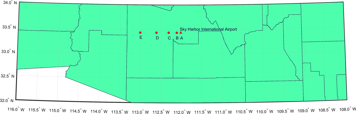
It is likely that two nearby aircraft use the same satellites in navigation. In this condition, the position errors of the two aircraft are highly correlated and we expect that the separation error will not be significant. A simulation example is used to present the relationship between separation loss and fault magnitude when the two aircraft are using the same set of GPS satellites, which includes one aircraft at point B, C, D and E, respectively. Another aircraft is fixed at point A that is close to the Sky Harbor International airport of Phoenix, Arizona (see Figure 3). The main parameters used in the simulation are illustrated in Table 2. As mentioned before, the clock and ephemeris error, tropospheric delay, ionospheric delay, multipath error and receiver noise are assumed to be Gaussian distributions. The same random variables are used to represent satellite ephemeris and clock errors (represented by σ _URE and σ _URA) at the same time for the two aircraft. The other error sources are assumed to be independent for the aircraft for conservative consideration.

Figure 3. Locations of the two aircraft that use the same satellite set to navigate. One aircraft is located at point A and the other is located at point B, C, D, E respectively to represent four scenarios.

Table 2. Parameters for simulation

Note: θ is the elevation angle from receiver to the corresponding satellite

Faults of magnitude from 0 to 1,000 metres were added to the visible satellites. The position errors of points A to E are presented in Figure 4, which indicates that satellite fault can cause considerable error at each point. The separation error (difference between surveillance separation and real separation) of the four scenarios were calculated from points B to E, which is shown as Figure 5. Note that the positive value representing the surveillance separation is greater than the real separation.

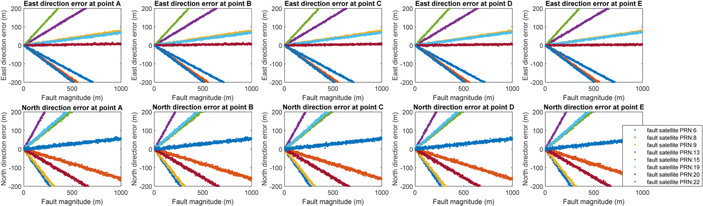
Figure 4. Separation loss versus magnitude of fault in each visible satellite

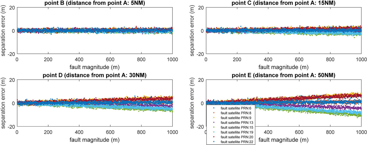
Figure 5. Separation loss versus magnitude of fault in each visible satellite.

The results indicate that satellite fault has little effect on separation error of the two aircraft when one aircraft is close to the other, for example, at point B. The satellite fault effect increases when the distance between the two aircraft increases. Note that large errors up to 1,000 metres are extreme scenarios that can be easily detected and excluded by the navigation receiver. The simulation in Figure 5 is to illustrate the effect of a satellite fault on separation error when the aircraft use the same satellite set to navigate. Such a large error is not realistic and is only used to demonstrate that even a large fault does not introduce a large separation error of the two aircraft (for example, all less than 20 m in the current simulation example).

4.2. Separation error analysis when aircraft use different satellite sets

Nearby aircraft may use different satellite sets for navigation due to various reasons. For example, some satellites may be blocked for one aircraft by terrain but can be used by the other aircraft that flies nearby. Figure 6 illustrates an example of this in the San Francisco terrain. The terrain data was developed by HUMUSOFT s.r.o. and The MathWorks, Inc (https://www.mathworks.com/help/sl3d/examples/terrain-visualization.html). The key parameters of this example are shown in Table 3.

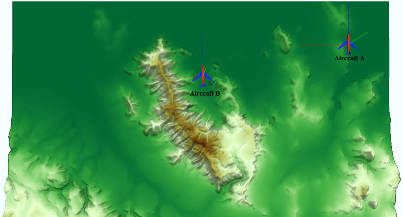
Figure 6. Illustration of how terrain could cause different satellite sets to be used by two nearby aircraft.

Table 3. Parameters for simulation.

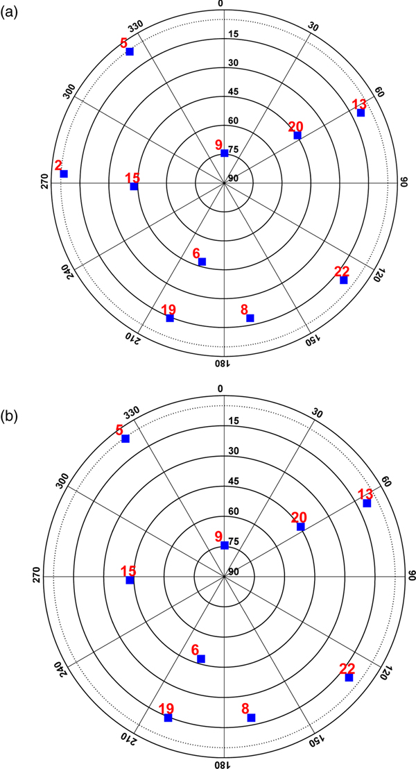
The contour lines of elevation angles for the terrain in this scenario are shown in Figure 7, which indicates that the terrain does not block positive elevation angles of aircraft A but blocks up to 10^° elevation angle of aircraft B. As a result, satellite #2 is blocked by the terrain in the view of aircraft B. The sky-plots are shown in Figure 8, where satellite #2 appears in the view of aircraft A but disappears from the view of aircraft B.

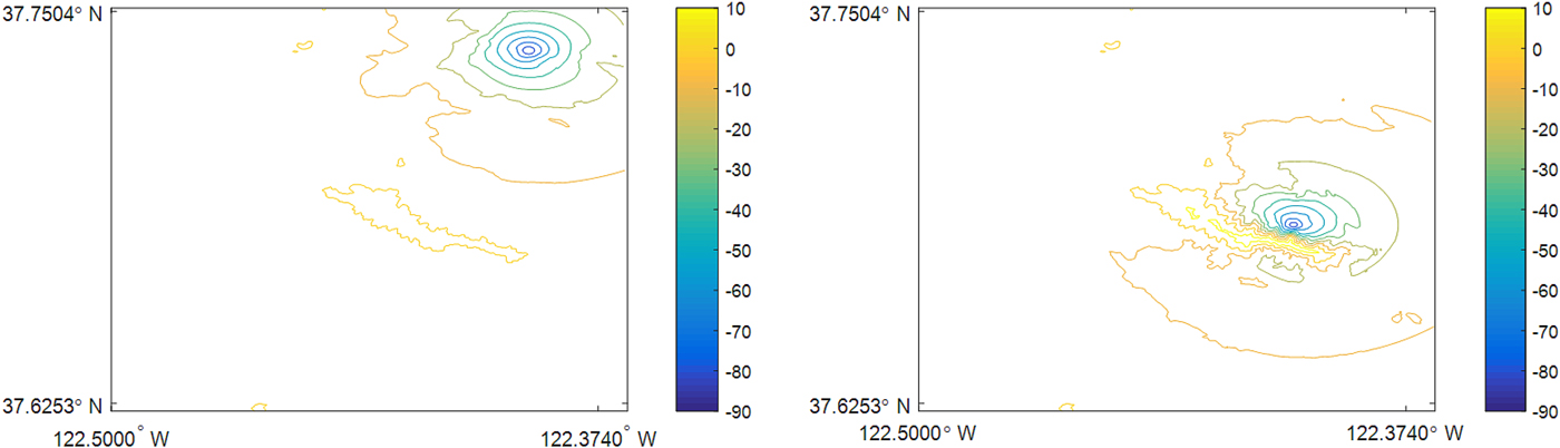
Figure 7. Contour lines of elevation angles for the two aircraft.

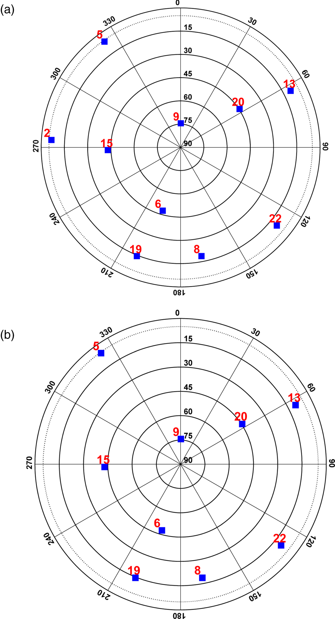
Figure 8. Sky-plots of aircraft A and aircraft B.

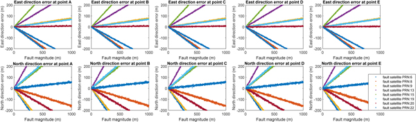
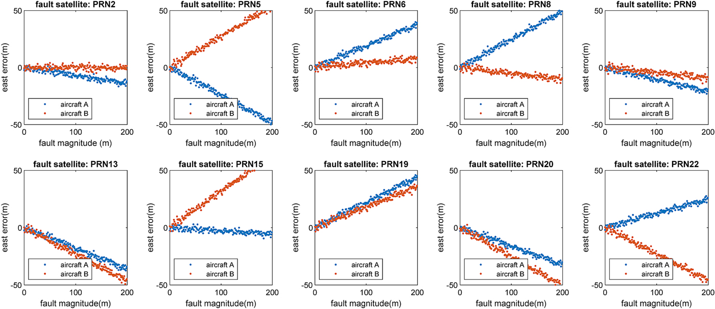
Fault magnitudes from 0 to 200 m were added into every visible satellite respectively to present the different effect on position errors of the two aircraft. The results of horizontal position error represented by east direction error and north direction error are shown in Figures 9 and 10, respectively.

Figure 9. Simulation results of fault effects on horizontal position (east direction) errors of the two aircraft.

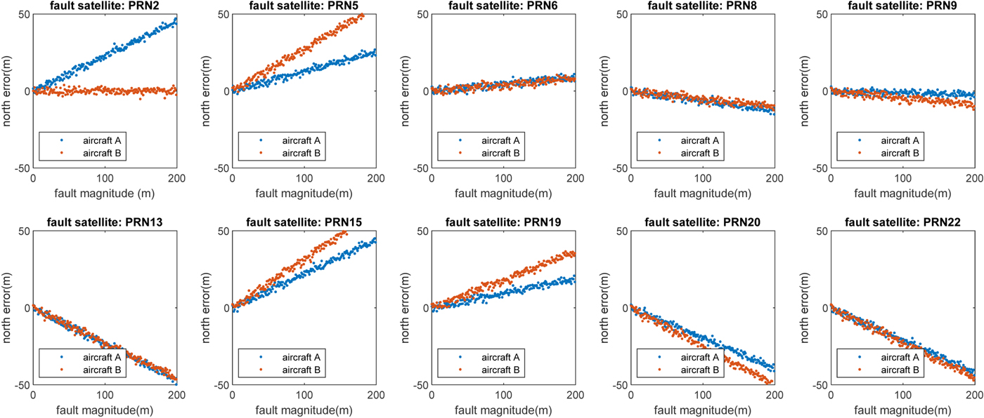
Figure 10. Simulation results of fault effects on horizontal position (north direction) errors of the two aircraft.

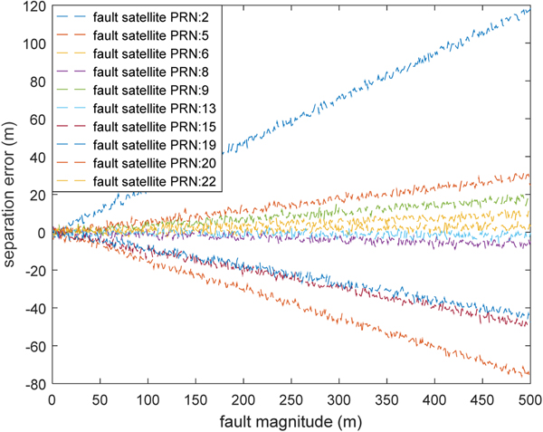
The simulation results demonstrate that if two aircraft see different satellite sets, then a fault occurring in a satellite could cause very different position errors on the two aircraft. The difference in positioning error could lead to a separation error. The results are illustrated in Figure 11 with different fault magnitudes.

Figure 11. Separation error versus fault magnitude in each visible satellite.

Figure 11 indicates that the fault in most of the visible satellites could cause a separation error. The largest loss is caused by satellite PRN #2. It is dangerous if the error is positive because the surveillance separation is larger than the real separation between the two aircraft. This simulation example demonstrates that the satellite information is critical in evaluating the separation error and should be broadcast.

4.3. Time-dependent separation loss probability assessment

The previous discussion was focused on the risk assessment in a “snapshot” manner. Due to the complex movement of satellites and aircraft, the separation loss probability is time-dependent in nature. An extension of the previous discussion is performed in this section for a 24-hour period. To simplify the discussion, we only consider the movements of satellites and focus on a specific location risk. Key parameters of the simulation are shown in Table 4. It is assumed that the satellite fault probability is 10⁻⁵, which is widely used in GNSS integrity analysis. This probability is based on the notion that there are “three service failures per year lasting no more than six hours” as specified in the GPS Standard Positioning Service Performance Standard (US DoD, 2001). The separation loss probability was evaluated under the assumption that the two aircraft used different satellite sets for navigation.

Table 4. Separation loss probability evaluation simulation parameters

Figure 12 shows the simulation results for different protection distance between aircraft A and aircraft B over a 24-hour period. The separation loss probability varies at different times of the day, and it decreases with the increase of protection distance.

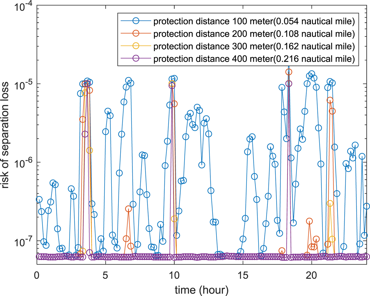
Figure 12. 24-hour time varing probability of separation loss for different protection distance.

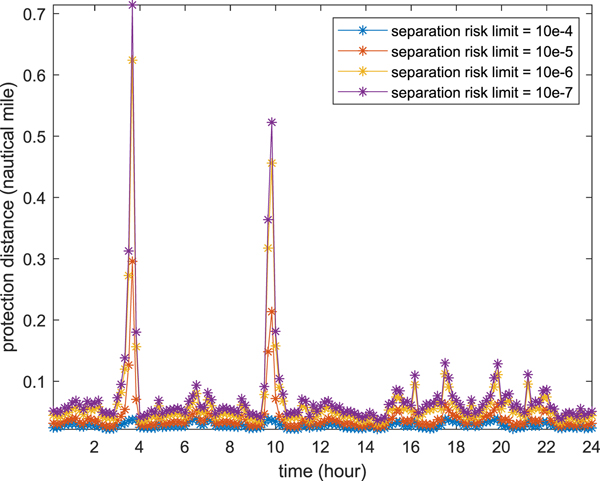
Another metric is used to illustrate the same results. Separation distance with a certain allowable risk level (that is, separation loss probability) is plotted with respect to time. As expected, a very high protection distance is required if the separation loss probability level needs to be maintained at a very low level (see Figure 13 for the probability level of 1e-7). This metric will be helpful for future decision making when the ADS-B signal is used for collision avoidance systems. It is shown that the high-risk scenarios only happen for a sparse number of time slots. It is too conservative to use these extreme cases to set the separation clearance. Thus, real-time separation loss probability assessments and dynamic separation clearance will be the ideal case for NextGen operation with the ADS-B system and its associated collision avoidance system.

Figure 13. 24-hour time varing protection for different separation loss probability limit.