1. Introduction
Growing concern over climate change and energy security has prompted governments to provide a variety of subsidy instruments at multiple levels in the renewable energy industry. For instance, many developed countries offer feed-in tariffs to firms and consumers who generate energy from renewable sources, and direct capital subsidies for large-scale renewable energy projects (IEA, 2013). However, governments often face political opposition to output subsidies to renewable energy, especially during periods of low economic growth (Stokes, Reference Stokes2013; Cherry et al., Reference Cherry, Kallbekken and Kroll2014). In such cases, policy-makers may alternatively pursue environmental goals through indirect means, such as entry policies (e.g., entry permits, subsidies, grants and low-interest loans), which facilitate development, increase competition and drive the price of emerging technologies down.Footnote 1 Our paper examines the welfare benefits of entry policy as an indirect form of environmental policy. We show that, relative to unregulated settings, domestic entry policies are welfare improving, and international policy coordination across countries yields a further increase in welfare. More surprisingly, however, we demonstrate that the welfare gain from promoting international policy coordination can be so small that it may not offset the costs from negotiating international agreements. This result suggests that countries should avoid international treaties that try to harmonize environmental entry subsidies when external benefits are small.
We analyze environmental entry policy by studying a two-stage game where, in the first stage, two regulators (one in each region) choose an entry policy to maximize domestic welfare. In the second stage, observing the entry policy, firms choose whether to enter and, if so, the region in which to enter and subsequently compete as Cournot oligopolists. Entering firms produce a relatively clean good, which can exhibit different degrees of environmental benefits. We consider two forms of entry policy: a permit restriction policy that acts like a quota on entry, and an entry tax or subsidy. In addition, we analyze each policy under three different scenarios: (1) both regions are unregulated; (2) each region autonomously regulates firms located within its jurisdiction; and (3) both regions coordinate regulation (social optimum). We then evaluate the stability of each equilibrium under the permit and entry tax/subsidy policy, and compare the welfare implications of the different regulatory structures.
First, we show that, while entry policy can be used to achieve environmental goals in a closed economy, free-riding and business-stealing effects arise under an international setting, thus precluding each regulator from reaching the social optimum when it independently sets its own subsidy policy. When environmental benefits are small, regulators would each prefer to restrict excessive entry (and thus capital investments in a closed economy), but they tend to relax entry when operating in an open economy in order to ‘steal business’ from the rival region. In contrast, when environmental benefits are large, a single regulator subsidizes a fraction of the socially optimal entry while its rival enjoys the benefits without subsidizing entry itself. We nonetheless demonstrate that, in both contexts, international policy coordination solves the business-stealing and free-rider problem that results from each regulator strategically setting entry policy.
Second, we find that the welfare gains of policy coordination are always positive, but depend critically on the product's environmental benefit. This result is particularly important since policy coordination requires costly negotiation of international agreements (Hovi et al., Reference Hovi, Ward and Grundig2014). In particular, we show that free-riding incentives are relatively small when environmental benefits are low. Consequently, a large share of welfare gains from international policy coordination can be achieved through optimal domestic (uncoordinated) regulation. By contrast, when environmental benefits are large, international policy coordination entails large welfare gains beyond those of optimal domestic policies.
As a consequence, our findings predict large welfare benefits from international agreements that harmonize subsidy policy in extremely clean industries, such as solar panels and wind turbines.Footnote 2 In contrast, our results show small welfare gains from coordinating policies in less clean industries, such as the production of corn-based ethanol.Footnote 3 If international negotiations are particularly costly, the welfare benefits of policy coordination in these industries may not justify the effort. Furthermore, our results suggest that, while international treaties are not necessarily desirable in certain contexts, the welfare gains of domestic (uncoordinated) policies are sufficiently large to recommend their introduction under a large set of parameter conditions. This result may apply to developing countries that are often reluctant to participate in international environmental agreements, such as nations in the G77 group during the negotiations in Rio de Janeiro 1992 and Johannesburg 2002. Although their non-participation is deemed as detrimental, our findings indicate that domestic policies can generate large welfare benefits.
Related literature. Over the past several decades, the WTO has actively discouraged countries from using strategic trade policies to promote domestic firms. As environmental policy began to gain acceptance, concern over the strategic use of environmental policy grew (Whalley, Reference Whalley1991; Barrett, Reference Barrett1994). A large literature has since analyzed the strategic use of emission standards and fees and the subsequent welfare impacts of such policies.Footnote 4 Most recently, Mason et al. (Reference Mason, Barbier and Umanskaya2014) explored the use of feed-in tariffs and border taxes as an indirect form of environmental regulation. While this literature has considered various environmental policies under both exogenous and endogenous market structures, it has largely overlooked the strategic use of entry policies in a multi-region economy with an endogenous market structure.Footnote 5
This paper lies at the intersection of a literature on strategic environmental policy and tax competition. The early literature on strategic policy demonstrates that governments may promote the competitiveness of domestic firms in imperfectly competitive international markets with R&D subsidies (Spencer and Brander, Reference Spencer and Brander1983) export subsidies (Brander and Spencer, Reference Brander and Spencer1985), import tariffs (Brander and Spencer, Reference Brander and Spencer1981) and domestic taxes and subsidies (Eaton and Grossman, Reference Eaton and Grossman1986). Afterwards, Barrett (Reference Barrett1994), Kennedy (Reference Kennedy1994); and Ulph (Reference Ulph1996), among others, extended the analysis to include environmental policy in an open economy. The common theme in this literature suggests that environmental policy in an open economy is likely not first-best because regulators fail to internalize market power as well as environmental externalities.
Several studies have since extended the literature on strategic environmental and trade policy to include endogenous entry in response to changes in policy (Katsoulacos and Xepapadeas, Reference Katsoulacos and Xepapadeas1995; Bhattacharjea, Reference Bhattacharjea2002; Bayındır-Upmann, Reference Bayındır-Upmann2003; Greaker, Reference Greaker2003; Fujiwara, Reference Fujiwara2009; Haufler and Wooton, Reference Haufler and Wooton2010; Etro, Reference Etro2011). This literature focuses almost exclusively on pollution externalities in production and the emission fees and standards used to control them. In contrast, we investigate an indirect environmental policy that affects industry structures and welfare and entry subsidies and taxes.
In a closely related literature on tax competition, geographically distinct governments compete over the foreign direct investment and associated tax revenue from domestically located firms (Zodrow and Mieszkowski, Reference Zodrow and Mieszkowski1986; Wilson, Reference Wilson1999). Janeba (Reference Janeba1998) develops a two-region model without environmental externality to show that even small tax differentials between regions can impact tax revenues due to firm relocation. Markusen et al. (Reference Markusen, Morey and Olewiler1995) study this phenomenon in the context of environmental regulation of pollution externalities and finds that each region relaxes regulation to attract entry. Our analysis also finds that welfare in each region is heavily dependent on firm location, which responds to differentials in entry policy. We then take the analysis a step further and show that the welfare benefits of international regulatory coordination diminish as environmental benefits rise, and can become smaller than the welfare gain of introducing domestic (uncoordinated) regulation.
The paper proceeds as follows. Section 2 analyzes a two-region model and establishes the optimal level of entry under various levels of coordination. Section 3 examines the equilibrium entry when the regulators use two different types of entry policies (quantity-based and price-based policy). Section 4 compares the welfare of the optimal entry level under various levels of coordination. Section 5 concludes with a discussion of the welfare gains of policy coordination.
2. Model
Consider a model of a two-region economy in which goods and services flow freely between regions A and B. Entry is endogenous and, upon entry, firms pay a region-specific fixed irrecoverable cost F k > 0, where k = {A, B}. This cost represents research and development as well as administrative costs necessary to enter the market and operate in region k. Firms in regions A and B face a world inverse demand P(Q) = a − bQ, where Q denotes total output of a clean product. Formally, each region has a demand function, P A(Q A) = a − b AQ A and P B(Q B) = a − b BQ B where b A = b/γ, b B = b/(1 − γ) and γ ∈ [0, 1], which aggregates to the world demand as detailed in appendix A1. The parameter γ determines the share of output consumed in region A, Q A(x, y) = γ Q(x, y), and region B, Q B(x, y) = (1 − γ) Q(x, y). All firms have symmetric marginal production costs, c.Footnote 6 Every firm in region k = {A, B} simultaneously and independently chooses output to maximize profits given the behavior of other firms, q k(x, y) = (a − c)/b (1 + x + y) where x and y denote the number of firms in regions A and B, respectively. We adopt the post-entry assumptions in Ruffin (Reference Ruffin1971) and Mankiw and Whinston (Reference Mankiw and Whinston1986): 1) the number of firms is a continuous variable, 2) additional entry reduces individual firm output, 3) additional entry increases aggregate industry output, and 4) the market price is greater than or equal to marginal cost. The equilibrium profits of a representative firm located in any region k = {A, B} are π k(x, y) = (a − c)2/b (1 + x + y)2, which are also decreasing in the number of entrants.Footnote 7 Therefore, a firm enters if π k(x, y) − F k ≥ 0. To guarantee the entry of at least one firm, we assume that the fixed entry cost is not prohibitive, i.e., π k(1) ≡ F max ≥ F k.
2.1 Unregulated entry
When regulation is absent (henceforth referred to as the ‘unregulated equilibrium’ and indicated by U), firm location is determined solely by the fixed entry cost, since there are no transportation costs and consumers perceive the goods to be perfect substitutes. If entry costs are lower in region A (B), all firms enter region A (B, respectively). If the entry cost coincides in regions A and B, firms are indifferent between operating in either region, as the next lemma describes. All proofs are relegated to the appendix.
Lemma 1
The unregulated equilibrium number of entrants in regions A and B solves π k(x, y) − F k = 0 where k = {A, B}, and is given by the (x, y)-pair
 $$(x^U,y^U)= \left\{\matrix{x=n^U, y=0 \hfill & {\rm if } F^A<F^B \hfill \cr (x,y) \hbox{ s.t. } x + y = n^U \hfill & {\rm if } F^A=F^B \hfill \cr x=0, y=n^U \hfill & {\rm if } F^A>F^B \hfill}\right.$$
where  $n^U \equiv ({a - c})/{\sqrt {b\min \{F^A,F^B\}} }-1$.
When the entry costs are symmetric across regions (i.e., F A = F B), every (x, y)-pair that satisfies x + y = n U is a possible equilibrium (see A2 for details). For simplicity, we focus on the symmetric equilibrium in which x U = y U = 1/2n U. When entry costs are lower in one country, all n U firms enter the low-cost region.
2.2 Coordinated entry
Consider a regulator whose jurisdiction spans regions A and B, i.e., an international organization coordinating entry in regions A and B. The regulator can control the entry of firms but not their behavior once they enter (also known as second best structural regulation by Vives (Reference Vives2001)). The optimal level of entry in regions A and B maximizes,
 $$\eqalign{W(x,y) & = CS(Q(x,y)) + \sum_i^x \{ \pi_i^A (x,y) - F^A\} \cr & \quad + \sum_j^y \{ \pi_j^B (x,y) - F^B\} + d Q(x,y)},$$
where CS(Q(x, y)) is total consumer surplus across both regions,  $\pi _i^k (x,y) - F^k$ is the profit of firm i in region k net of any fixed entry costs, and d ≥ 0 is the marginal benefit of consuming clean products.Footnote 8 In the case of energy, d represents the marginal benefits of installing renewable energy technologies, i.e., solar panels and wind turbines, in either region. Alternatively, these benefits arise from the substitution away from technologies that create environmental damage.
The first-order conditions with respect to the number of firms x and y are
 $$W_x: \quad CS_Q Q_x(x,y) + (\pi^A(x,y) - F^A) + dQ_x(x,y) = x\pi^A_x(x,y) + y\pi^B_x(x,y)$$
 $$W_y: \quad CS_Q Q_y(x,y) + (\pi^B(x,y) - F^B) + dQ_y(x,y) = y\pi^B_y(x,y) + x\pi^A_y(x,y),$$
where the subscripts denote partial derivatives, that is, CS Q ≡ ∂CS/∂Q,  $Q^k_x \equiv \partial Q^k/ \partial x$, and
  $\pi ^k_x \equiv \partial \pi ^k/ \partial x$ where k = {A, B}. The symmetry of firms implies
  $\sum \nolimits _i^x \pi _i^A (x,y)=x\pi ^A (x,y)$ and in a slight abuse of notation, we now use the subscript to denote the partial derivative. The left hand side of (3) and (4) represents the benefit of an additional entrant including: the increased consumer surplus due to a larger aggregate output, the net profits of the new entrant, π k − F k, and the benefits associated with an increase in the domestic consumption of clean goods. Each of these three terms is positive, but diminishing in x and y. In contrast, the right hand side of the first-order condition represents the dissipation of aggregate profits in regions A and B due to new entry, which is positive and decreasing in x and y. The socially optimal (SO) level of entry in regions A and B solves (3) and (4) and is given by (x SO, y SO).
The single regulator, who coordinates entry in both regions, is indifferent between entry in regions A and B because they are symmetric and transportation costs are zero. If the entry costs are lower in one region, welfare maximizing entry requires that all firms enter into the low-cost region. Alternatively, if entry costs are equal, the regulator allocates firms to both regions evenly. In order to facilitate the comparison of the socially optimal entry, (x SO, y SO), and the unregulated entry, let n SO = x SO + y SO be the aggregate number of firms that solves
 $$CS_n(n) + (\pi(n) - F) + dQ_n(n) = n\pi_n(n)$$
where CS n = CS x = CS y, π = π A = π B, F = min{F A, F B},  $Q_n=Q^k_x=Q^k_y$, and
  $n\pi _n=x\pi ^A_x=y\pi ^B_x=y\pi ^B_y = x\pi ^A_y$.Footnote 9 Lemma 2 compares the socially optimal number of firms, n SO, (arising from the presence of a regulator coordinating entry policies across regions) against the unregulated equilibrium number of firms, n U.
Lemma 2
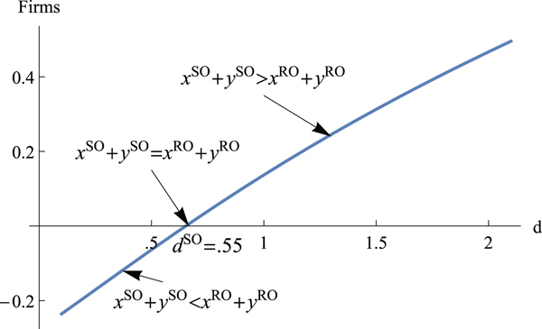
The unregulated level of entry exceeds the socially optimal level of entry, n U > n SO (or x U + y U > x SO + y SO), if and only if n π n(n U) > CS n(n U) + dQ n(n U), or alternatively, when goods are not sufficiently clean, i.e., d < d SO where  $d^{SO} \equiv a-c - \sqrt {bF}$.
We illustrate the result of lemma 2 in figure 1 using a parametric example.Footnote 10 In particular, it depicts cutoff d SO in (F, d)-space, where unregulated and socially optimal entry coincide, i.e., n U = n SO. When the environmental benefit is below d SO for a given value of F, unregulated entry exceeds the socially optimal entry because profit dissipation decreases welfare more than the environmental benefits of increased production. In contrast, environmental benefits above d SO increase the social value of output relative to dissipated profits, which lead the regulator to encourage entry. If the unregulated and socially optimal level of entry do not coincide (n U ≠ n SO), the regulator can use entry policy to induce the socially optimal level of entry. We describe this result in section 3.3.
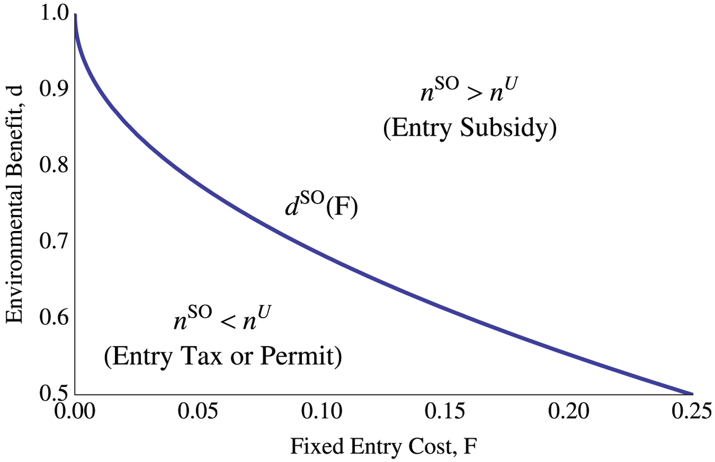
Figure 1. Comparing socially optimal and unregulated entry.
2.3 Uncoordinated entry
This section examines the optimal level of entry that arises when regions A and B do not coordinate. We consider two regions that are still symmetric in production, entry costs and marginal benefit of consuming clean products to facilitate the comparison of uncoordinated and coordinated optimal entry in both regions. If each regulator could choose the number of firms within its jurisdiction conditional on the number of firms in the rival region, they would maximize
 $$[{\rm Regulator} \,A] \quad W^A(x,y) = CS^A(Q^A(x,y)) + \sum_i^x \{ \pi_i^A (x,y) - F^A\} + d Q^A(x,y)$$
 $$[{\rm Regulator} \,B] \quad W^B(x,y) = CS^B(Q^B(x,y)) + \sum_j^y \{ \pi_j^B (x,y) - F^B\} + d Q^B(x,y).$$
The region-specific welfare functions are similar to the welfare function introduced in equation (2) but do not account for the benefits or costs imposed on the other region. Importantly, consumer surplus, CS k(Q k(x, y)), and the environmental benefit, d Q k(x, y) for k = {A, B}, only accrues to the domestic economy. This welfare specification represents situations in which environmental benefits are localized (e.g., improvement in water quality).Footnote 11 Thus, the first-order conditions of regulator A and B are
 $$[{\rm Regulator} \,A] \quad W^A_x:\quad CS^A_{Q^A} Q^A_x(x,y) + \pi^A (x,y) - F^A + dQ^A_x(x,y) = x\pi^A_x (x,y)$$
 $$[{\rm Regulator} \,B] \quad W^B_y: \quad CS^B_{Q^B} Q^B_y(x,y) + \pi^B (x,y) - F^B + dQ^B_y(x,y) = y\pi^B_y (x,y).$$
The first-order conditions implicitly characterize the regulator's best response functions, x(y) and y(x), which are illustrated in figure 2.Footnote 12 Each region's best response function is decreasing, which implies that each regulator perceives entry in the other region as a strategic substitute for domestic entry. For example, region A would promote a smaller number of domestic firms as more firms enter region B. The rationale behind such a strategy is the well-known free-riding argument across jurisdictions. As more firms enter region B, the increase in aggregate production benefits consumers in region A, despite eroding domestic profit. Hence, the regulator in region A can free-ride off of these benefits, ultimately supporting the entry of fewer firms into his own jurisdiction. Since regions are symmetric, the results hold for region B as well.Footnote 13 The intersection of the best response functions in figure 2 indicates the regionally optimal (RO) level of entry, (x RO, y RO). If both regulators can induce this level of entry using taxes, subsidies or permits, then the intersection becomes a candidate for the two-region regulated equilibrium. We further investigate this equilibrium in section 3.
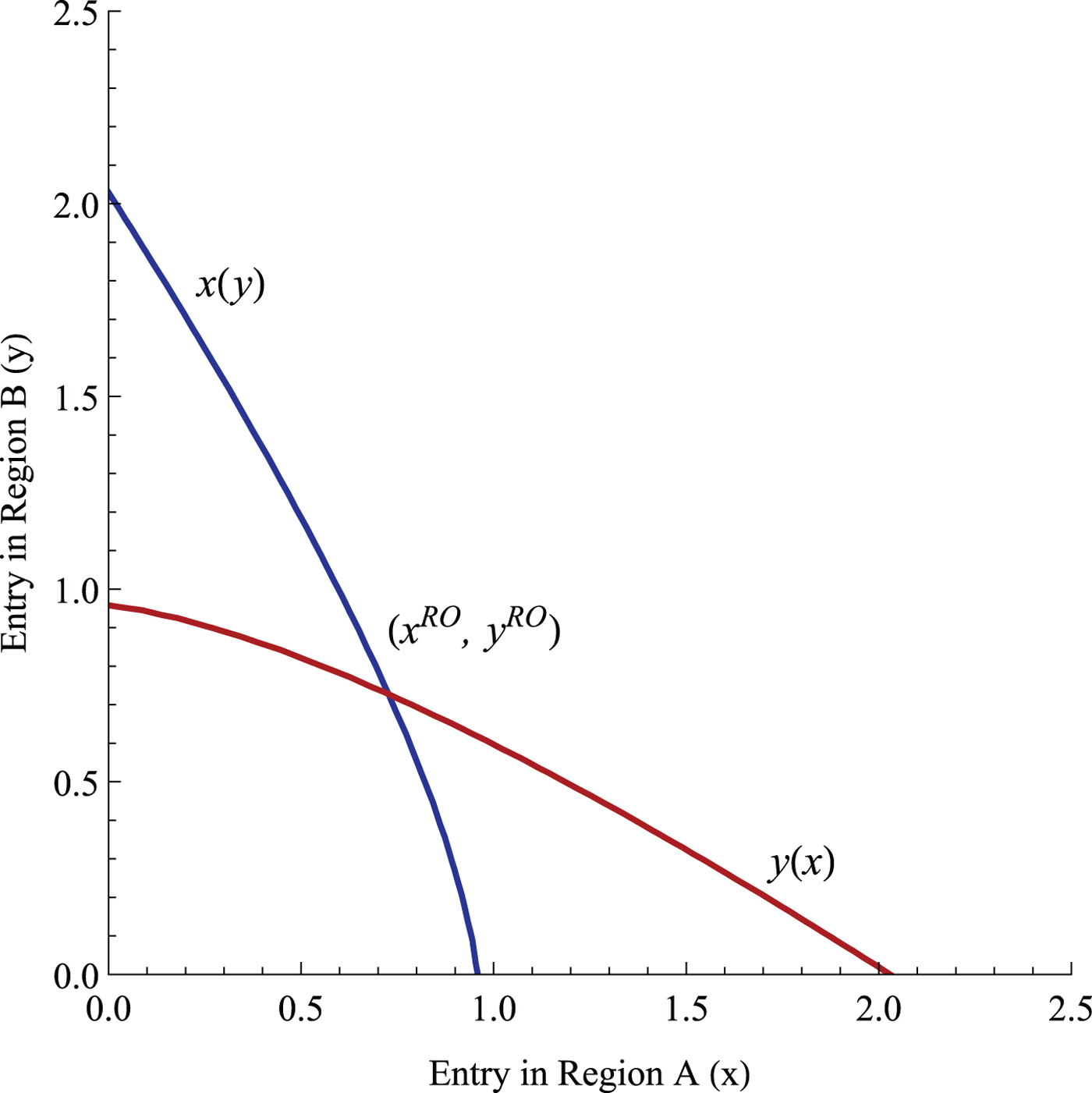
Figure 2. The regulators' best response functions in regions A and B.
2.3.1 Entry externalities.
The regionally optimal entry (x RO, y RO) does not necessarily coincide with the socially optimal entry (x SO, y SO) of section 2.2. Specifically, entry in region k = {A, B} creates two forms of externality in region ℓ ≠ k: on the one hand, it increases competition among firms, thus dissipating profits but it also increases consumer surplus.Footnote 14 Conventional positive externalities arise from the increased production of clean products in the foreign region, which benefits all regions when consumed (or installed in the case of solar panels). These externalities are evident when comparing the first-order conditions of the single regulator in section 2.2 (in equations (3) and (4)) to those of the two separate regulators in section 2.3 (in equations (8) and (9)). If regulator A increases entry in region A, it does not account for the positive externalities  $(dQ^B_x + CS^B_{Q^B} Q^B_x(x,y))$ or negative externalities
  $(y\pi ^B_x)$ it imposes on region B's welfare.
The next lemma evaluates the range of environmental benefit, d, for which the regionally optimal number of firms is larger than the unregulated number of firms for each region, i.e., x RO > x U and y RO > y U. The proof of lemma 3 is in appendix A5.
Lemma 3
The regionally optimal level of entry exceeds the unregulated level of entry in region A, x RO > x U (in region B, y RO > y U), if and only if the benefits of consuming clean products are sufficiently high, i.e.,  $d^k>{\underline d}^k$, where
  $ {\underline d}^A \equiv {(1-\gamma )}/{\gamma } d^{SO}$ for region A; and
  ${\underline d}^B \equiv {\gamma }/{1-\gamma } d^{SO}$ for region B. Finally,
  $ {\underline d}^A < {\underline d}^B$ if and only if γ < 1/2.
Figure 3 depicts cutoffs  ${\underline d}^A$ and
  ${\underline d}^B$ as a function of the share of consumption in region A, γ. For completeness, the figure also includes cutoff d SO from lemma 2. Note that cutoff d SO does not depend on the geographic distribution of consumption, γ, when regulators jointly coordinate their entry policy. In contrast, cutoffs
  ${\underline d}^A$ and
  ${\underline d}^B$ are inversely related to their respective shares of domestic consumption (γ in region A and 1 − γ in region B) and divide the parameter space (γ, d) into four partitions that provide a comparison of unregulated entry relative to two regulatory benchmarks: socially optimal entry (coordinated policies) and regionally optimal entry (uncoordinated policies).
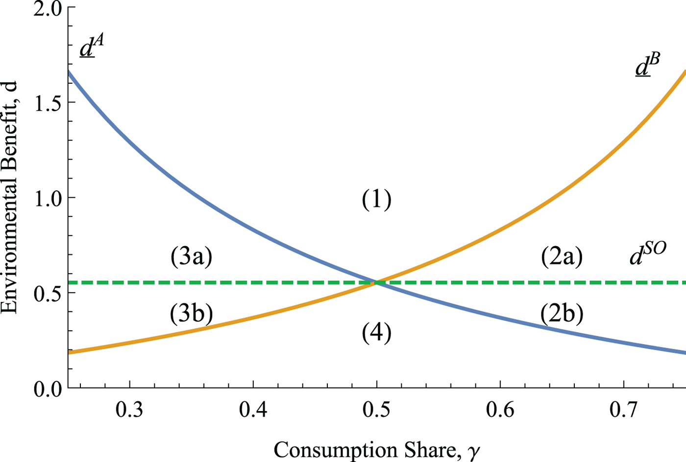
Figure 3. Cutoffs  ${\underline d}^A$ and
  ${\underline d}^B$ divide the (d, γ)-space into four partitions. Regulator k = {A, B} encourages entry above
  ${\underline d}^k$ and discourages entry below
  ${\underline d}^k$.
Partition (1) represents the case in which environmental benefits are large enough that both regulators promote entry beyond the unregulated equilibrium (x RO > x U and y RO > y U). This preference for increasing entry by each autonomous regulator coincides with their preferences when coordinating policies, i.e.,  $\max \{{\underline d}^A, {\underline d}^B\} \geq d^{SO}$. In partition (2), regulator A prefers to encourage entry (x RO > x U) while regulator B prefers to discourage entry (y RO < y U), given that
  ${\underline d}^B>d>{\underline d}^A$. Intuitively, region A benefits more from consumer surplus and clean products than the reduction in firm profits because γ > 0.5. Partition (2) is bisected by d SO. In (2a), coordinated regulation encourages entry relative to the unregulated equilibrium, i.e., x SO > x U and y SO > y U, whereas in (2b) the coordinated regulation limits entry. An opposite argument applies in partition (3), where only regulator B encourages entry (y RO > y U). As is the case in partition (2), the single regulator would increase entry in the region above cutoff d SO in partition (3a), and decrease entry below d SO in partition (3b). Finally, in partition (4), both regulators discourage entry (x RO < x U and y RO < y U), since the benefits of consuming clean goods are relatively low. The single regulator would also restrict entry in all of partition (4), i.e., x SO < x U and y SO < y U.
While our previous discussion compares unregulated entry against two regulatory benchmarks (SO and RO), we have not yet examined whether entry under uncoordinated regional policies (RO) is insufficient (relative to the social optimum, SO). We confirm this result in lemma 4.
Lemma 4
The socially optimal level of entry exceeds the regionally optimal level of entry in region A, x SO > x RO (in region B, y SO > y RO), when the marginal external benefits of entry to the other region exceed the marginal costs imposed on the other region  $CS^B_{Q^B}Q^B_x + dQ^B_x > y\pi ^B_x$ in region A
  $(CS^A_{Q^A}Q^A_y + dQ^A_y > x\pi ^A_y$ in region B, respectively), which holds for all d > d SO.
When the benefits of clean goods are sufficiently large (high d), entry increases welfare in the other region despite the dissipation of firm profits. Regionally optimal entry is smaller than the socially optimal entry because output is consumed in both regions, which implies that the benefits of more output are shared with the rival region and not completely internalized. Figure 4 depicts the difference between the socially optimal and regionally optimal aggregate level of entry, (x SO + y SO) − (x RO + y RO) in (x + y, d)-space using our parametric example when γ = 0.5. The figure shows that for d > d SO, the socially optimal entry exceeds the regionally optimal entry. The proof of lemma 4 is in appendix A6.
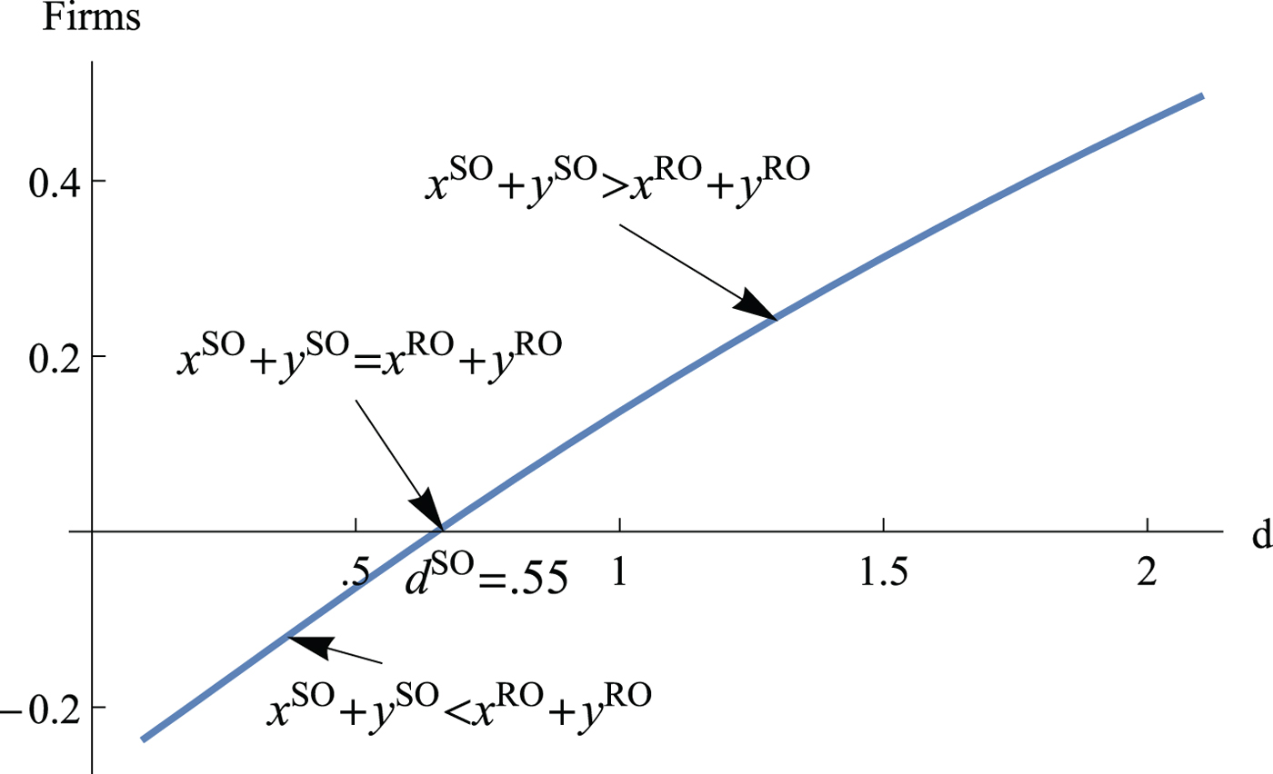
Figure 4. Difference between the socially optimal (SO) and regionally optimal (RO) aggregate entry as a function of d.
3. Entry policies
Throughout section 2.3 we took the regulators' ability to induce the regionally optimal level of entry as a given. We now explore whether the regionally optimal level of entry (x RO, y RO) can be implemented using either a quantity-based policy (i.e., entry permits) and a price-based entry policy (i.e., entry tax or subsidy). Price- and quantity-based instruments alter the incentives of potential entrants in different ways. Our discussion will focus on the incentive structure created when regulators are restricted to one of these policy types.
3.1 Quantity-based entry policy
Consider the case in which both regulators use a quantity-based entry policy such as permit restrictions. A permit policy allows regulator k to directly restrict entry in region k, but not to restrict entry in region ℓ ≠ k, where k = {A, B}.
Proposition 1
Under a quantity-based entry policy, both regulators limit the number of entrants and induce the regionally optimal level of entry, (x RO, y RO), if  $d \leq \min \{{\underline d}^A,{\underline d}^B \}$, but do not limit the number of entrants allowing for the unregulated level of entry to arise, (x U, y U), otherwise.
Proposition 1 establishes the equilibrium that emerges under the quantity-based policy instrument and is proved in appendix A7. The limitation of the permit policy to only restrict entry implies that it is only effective when the regulators in each region find it optimal to restrict entry (in partition (4) of figure 5). Partition (4) represents the (d, γ)-pairs where the RO policy calls for both regulators to restrict entry, i.e., (x RO, y RO) < (x U, y U). Therefore, regulator A (B) sets a permit limit equal to x RO (y RO, respectively). Neither regulator has incentive to deviate from this strategy because x RO (y RO) maximizes the welfare in region A (B, respectively) and thus, relaxing the policy to encourage entry would decrease welfare. In partitions (1-3), at least one regulator would like to encourage entry, which implies that they would not limit available permits. If regulator A does not use permits to restrict entry, regulator B cannot benefit by restricting entry because the firms that would have been prevented from entering region B locate in region A instead resulting in (x U, y U).
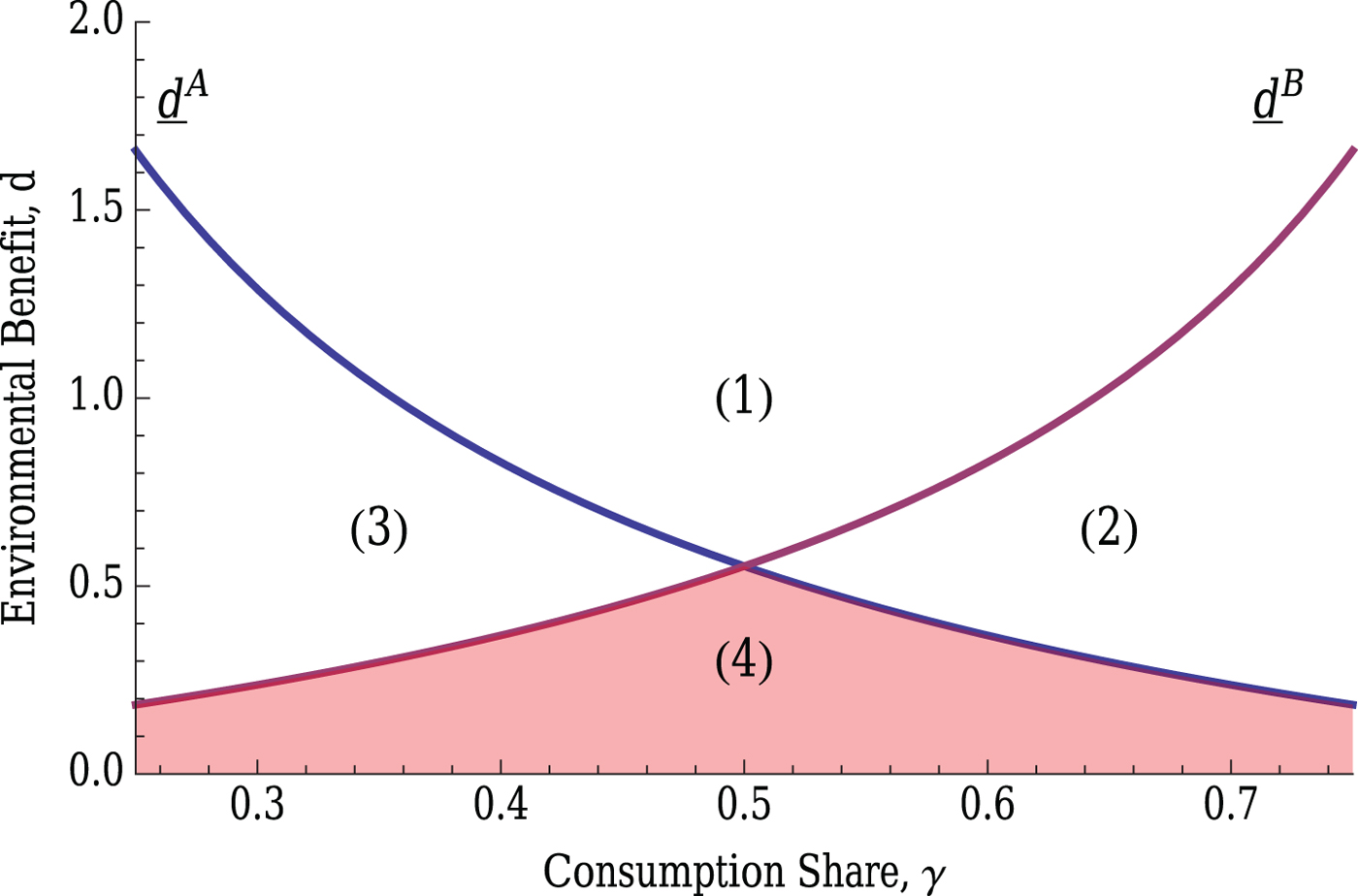
Figure 5. Cutoffs  ${\underline d}^A$ and
  ${\underline d}^B$ divide the (d, γ)-space into four partitions characterized by the regulators preference for entry. The shaded area indicates the conditions under which the regionally optimal level of entry, (x RO, y RO), can be implemented with a quantity-based entry policy.
3.2 Price-based entry policy
Regulators may instead promote RO with entry taxes or subsidies. As described in lemma 3, the regionally optimal entry is less than the unregulated number of firms, (x RO, y RO) < (x U, y U), when the benefit of clean products is low, which suggests that regulators could hinder entry with a tax. In contrast, the regionally optimal number of firms exceeds the unregulated number of firms, (x RO, y RO) > (x U, y U), when the benefits of clean products are sufficiently high, suggesting the use of subsidies to encourage entry. However, price-based entry policies pose an administrative challenge in a strategic context because both regulators have an incentive to deviate from the strategy that induces (x RO, y RO). Proposition 2 describes the equilibrium under a tax/subsidy policy as a function of the environmental benefit, d.
Proposition 2
Under a price-based entry policy, both regulators set a zero tax, z A = z B = 0, and thus induce the unregulated equilibrium level of entry (x U, y U) if  $d < \min \{ \hat {d}^A, \hat {d}^B \}$; and only regulator A (B) sets a subsidy
  $\hat {z}^A<0\,(\hat {z}^B<0)$ to induce n R entrants in region A if
  $d \geq \hat {d}^A$ and γ ≥ 0.5 (or in region B if
  $d \geq \hat {d}^B$ and γ < 0.5, respectively).
Price-based entry policies threaten the implementation of RO by creating the incentive to deviate from the conditionally optimal strategy. We characterize the regulator's incentive to deviate over three distinct ranges of environmental benefit, each depicted in figure 6: 1)  $d \leq \min \{{\underline d}^A,{\underline d}^B \}$, 2)
  $\min \{\hat {d}^A,\hat {d}^B \} \geq d > \min \{{\underline d}^A,{\underline d}^B \}$, and 3)
  $d > \min \{\hat {d}^A,\hat {d}^B \}$.
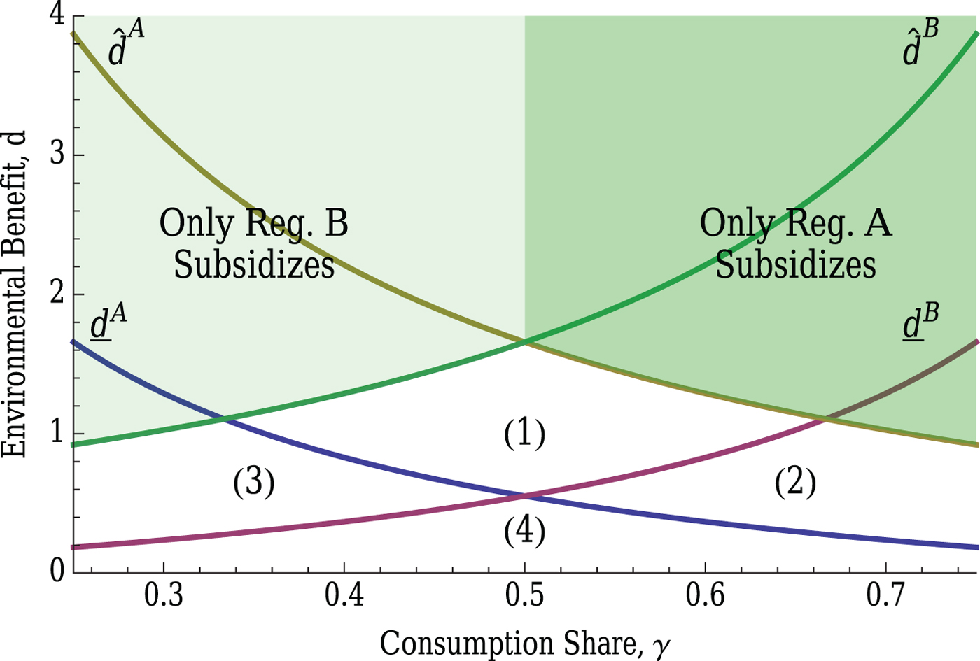
Figure 6. Cutoffs  ${\underline d}^A$ and
  ${\underline d}^B$ divide the (d, γ)-space into four partitions. Cutoffs
  $\hat {d}^A$ and
  $\hat {d}^B$ are defined in A8 and further divide the conditions under which regulators promote entry into conditions that sustain an entry subsidy equilibrium (when
  $d>\hat {d}^k$).
Partition (4) in figure 6 depicts the case where environmental benefits are low, i.e.,  $d \leq \min \{{\underline d}^A,{\underline d}^B \}$, and both regulators would prefer to deter entry by setting an entry tax to achieve (x RO, y RO). However, each regulator knows that he can relax his own entry tax thereby attracting all firms into his own region and increasing welfare through additional domestic profits. This result embodies a feature commonly noted in the literature on tax competition (Janeba, Reference Janeba1998; Wilson, Reference Wilson1999), which assumes no environmental benefit, i.e., d=0. The incentive of both regulators to reduce entry taxes for any
  $d \leq \min \{{\underline d}^A,{\underline d}^B \}$ implies that they both set an entry tax equal to zero and the unregulated equilibrium prevails, (x U, y U).
Partitions (1)–(3) in figure 6 depict the case where environmental benefits are moderate,  $\min \{\hat {d}^A,\hat {d}^B \} \geq d > \min \{{\underline d}^A,{\underline d}^B \}$, and both regulators would now encourage entry by setting an entry subsidy to achieve (x RO, y RO) where (x RO, y RO) > (x U, y U). Despite the welfare gains from setting a subsidy to encourage (x RO, y RO), both regulators have the incentive to free-ride off of the other regulator's subsidy. If regulator A (B) reduces its subsidy, all firms enter into region B (A, respectively). Therefore, regulators set a subsidy of zero when environmental damages are moderate, resulting in the unregulated equilibrium, (x U, y U).
The shaded region in figure 6 depicts the case where environmental benefits are large,  $d>\min \{\hat {d}^A,\hat {d}^B \}$. In contrast to the case where free-riding prevents either regulator from providing subsidies, environmental benefits are high enough that at least one regulator subsidizes all entry. However, the fact that a portion of output is exported implies that the subsidizing region receives only a fraction of the benefits, which diminishes the incentive to subsidize. Therefore, the regulator who benefits the most (region A when γ ≥ 0.5, and region B when γ < 0.5) subsidizes entry to maximize domestic welfare conditional on zero entry in the other region.Footnote 15 Note that a price-based entry policy does not allow both regulators to reach the regional optimum (x RO, y RO), but instead, (x, y) = {(n R, 0), (0, n R), (x U, y U)} arise.
Our analysis examines an indirect form of regulation, i.e., entry policies, which may coexist with more direct regulation such as output-based emission fees and subsidies. Consider a production subsidy that reduces the marginal cost of production to  $\hat {c}=c-s$, where s>0 is a subsidy. A reduction in marginal cost raises the cutoff,
  $d^{SO} \equiv a-\hat {c}-\sqrt {bF}$, above which optimal entry exceeds the unregulated level of entry. As a consequence, the environmental benefit would need to be higher for the planner to encourage entry. Therefore, price-based entry policies are strategic sustitutes for direct production subsidies.
3.3 Socially optimal entry policies
We now consider whether coordinated entry policy can induce the socially optimal level of entry. Section 2.2 establishes the socially optimal level of entry n SO = x SO + y SO that maximizes equation (5). When regulation is coordinated, a permit policy can induce n SO if d ≤ d SO. The permit policy cannot induce n SO if d > d SO since firms cannot be coerced to enter the market.
In the case of the price-based policy, the regulators can coordinate to set an entry tax or subsidy, which is equivalent to choosing the number of entrants, x and y, to maximize aggregate welfare. Consider the welfare function:
 $$\eqalign{W(x,y) & \equiv CS(Q(x,y)) + \sum_i^x \{\pi_i^A (x,y) - (F^A +z)\} \cr & \quad + \sum_j^y \{ \pi_j^B (x,y) - (F^B+z)\} + (x+y)z + D(Q(x,y)),}$$
where z is the entry tax (z > 0) or subsidy (z < 0) and the other terms are as defined in equation (2). The government revenue (or cost) generated by the tax (or subsidy) is offset by the opposite effect on producer surplus. Consequently, this welfare function simplifies to equation (2) (Janeba, Reference Janeba1998).
When d < d SO and n SO < n U, the regulators can set a tax, z>0, which solves π(n SO) = F + z. This occurs, for instance, when no environmental benefit arises from the domestic consumption of the good, i.e., d=0, which is consistent with the results in Mankiw and Whinston (Reference Mankiw and Whinston1986) where the regulator limits entry by increasing entry costs. By contrast, when private entry is insufficient, n SO > n U or d ≥ d SO, the regulator may offer an entry subsidy z<0, which again solves π(n SO) = F + z, inducing additional entry.
4. Welfare
Coordination of policy, environmental or otherwise, across jurisdictions often involves costly negotiation. We compare the welfare gains of policy coordination to the uncoordinated policy equilibrium as well as the unregulated equilibrium to explore the merits of coordinated regulation. Table 1 contains the aggregate welfare benefits arising from the transition between regulatory settings i.e., from U to RO, and from RO to SO.Footnote 16
Table 1. Aggregate welfare (W = W A + W B) of each regulatory context: no regulation, uncoordinated regulation, and coordinated regulation under low, moderate and large environmental benefits. Welfare gains from moving between regulatory contexts are in parentheses (in percent change)

Policy coordination is always welfare improving because the external benefits of entry are internalized. The welfare gains of policy coordination increase as the environmental benefit rises. When the environmental benefits are low (d=0.3), permit restrictions can be used to implement the uncoordinated equilibrium, (x RO, y RO), and capture a large share of the welfare gains resulting from policy coordination (1.57 per cent increase versus 0.31 per cent). As benefits rise to a moderate level (d=1), free-riding prevents any successful uncoordinated regulation (RO); however, coordinated regulation (SO) increases welfare by 2.27 per cent. When environmental benefits are large (d=2), uncoordinated regulation (one region subsidizes all entry) only achieves a welfare increase of 2.94 per cent versus a 7.18 per cent increase from policy coordination. Therefore, policy coordination yields large welfare gains when environmental benefits are large and may be less critical when environmental benefits are small.
5. Discussion and conclusion
Insufficient or excessive entry? We study the use of entry policy as a form of indirect environmental regulation in an imperfectly competitive, multi-region setting. Our results show that, when positive environmental externalities are small or zero, entry is excessive (relative to the social optimum) both when entry is left unregulated and when it is independently regulated within each jurisdiction. Hence, entry subsidies are too generous when environmental benefits of the good are small. In contrast, when environmental benefits are large, entry is insufficient under the unregulated and autonomously regulated contexts, thus implying that entry subsidies are insufficient. As a consequence, the coordination of entry policies across regions can help approach entry patterns to the social optimum.
Policy coordination: Not always recommended. Policy coordination ameliorates the free-riding and business-stealing incentives by ensuring that externalities are internalized. While international policy coordination is welfare improving, its size crucially depends on the environmental benefit of the good. We find that for small environmental benefits, policy coordination yields a relatively negligible welfare increase. However, significant welfare gains can arise under moderate environmental benefits. In this case, policy coordination helps regions set more generous entry subsidies, thus promoting more entry than when each region independently sets its own policy. Interestingly, at very large environmental benefits, the welfare gains of uncoordinated policy exceed the gains of coordination.
Therefore, our findings indicate that, while introducing domestic regulation yields welfare gains (relative to unregulated settings), investing a large amount of resources to achieve international policy coordination is not necessarily beneficial. Specifically, countries should coordinate their subsidy policies in industries with moderate to large environmental benefits, such as solar panels and wind turbines, but should actually avoid costly negotiations in industries with relatively small environmental benefits, such as biofuels. This result argues against promoting policy coordination between the U.S. and Europe, as the U.S. is claimed to provide generous entry subsidies to its biofuel industry (e.g., loans for starting up companies). Intuitively, promoting further entry in this industry yields a small environmental benefit which, after a sufficient number of firms enter (either domestically or overseas), is offset by the profit dissipation incumbent firms suffer, ultimately yielding an overall welfare loss.
Do not overlook domestic policies. Our results also show that, in certain contexts, the percent increase in welfare arising from the introduction of domestic policy (i.e., from the U to RO setting) can be larger than that of further moving to international policy coordination (i.e., from RO to SO). Although both policy changes entail a welfare improvement, the latter is smaller under most parameter combinations. Intuitively, this indicates that, if international policy coordination is costly or politically difficult, countries can still accrue most of the policy benefits by at least introducing domestic policies, while avoiding international treaties.
Appendix A
A1 Demand aggregation
Regions A and B each have region-specific inverse demand functions, P A(Q A) = a − b AQ A and P B(Q B) = a − b BQ B. Aggregate demand is the sum of the quantity demanded across both regions at any price level:
 $$Q=Q^A+Q^B=\displaystyle{{a-P^A}\over{b^A}} + \displaystyle{{a-P^B}\over{b^B}}.$$
Without transaction costs, the price in each region should be equal across regions in equilibrium, i.e., P A = P B = P, which yields
 $$Q= (a - P) \left(\displaystyle{{1}\over{b^A}} + \displaystyle{{1}\over{b^B}}\right).$$
Solving for P, we obtain the inverse demand function
 $$P=a-\displaystyle{{Q}\over{{1}/{b^A} + {1}/{b^B}}}.$$
Define b A ≡ b/γ, where γ ∈ [0, 1] and b ≥ 0, and b B ≡ b/(1 − γ); we provide an economic interpretation of parameters γ and b below. Using these definitions, the above aggregate inverse demand function simplifies to
 $$P=a-\displaystyle{{Q}\over{{\gamma}/{b} + {1-\gamma}/{b}}}= a - bQ.$$
We can then express Q A as a share γ of aggregate output Q, as follows:
 $$Q^A=\displaystyle{{a-P}\over{b^A}}=\displaystyle{{\gamma (a-(a-bQ))}\over{b}}=\gamma Q.$$
An analogous argument holds for region B.
A2 Proof of lemma 1
Firms enter the region in which they earn the highest profit net of entry costs. Since firms compete in an interregional market, gross profits are independent of location in region A or B. Therefore, firms locate in the region with the lowest entry cost F k where k = {A, B}. There are three possible entry cost cases in the absence of regulation: 1) F A < F B, 2) F B < F A, and 3) F A = F B. In case 1, all firms enter region A and the equilibrium number of firms x U solves
 $$\pi^A(x,0)-F^A= \displaystyle{{(a-c)^2}\over{b(1+x)^2}} - F^A=0.$$
The equilibrium number of firms is  $x^U={a-c}/{\sqrt {b F^A}}-1$, and is equivalent to the equilibrium entry in a single region. Conversely, the equilibrium number of firms in case 2 solves an analogous equation where A=B and x=y, which yields
  $y^U={a-c}/{\sqrt {b F^B}}-1$. In case 3, the entry cost in both regions are equal (F ≡ F A = F B) and entrants are indifferent between entry in regions A or B. Therefore, entry in regions A and B, i.e., (x,y) solves n=x+y. Equilibrium entry n U solves
 $$\pi(n)-F= \displaystyle{{(a-c)^2}\over{b(1+n)^2}} - F=0$$
and is  $n^U={a-c}/{\sqrt {b F}}-1$. We confine our analysis to the nontrivial cases in which entry costs are not prohibitive (i.e., 0 ≤ F < F max ≡ (a − c)2/4b where F max is equal to the monopolist's gross profit). We summarize the three possible cases in a general representation of the unregulated equilibrium entry
  $n^U={a-c}/{\sqrt {b \min \{F^A,F^B\}}}-1$.
A3 Concavity of the welfare function
The number of entrants n SO maximizes W(n) if it solves W n = 0 and W nn < 0. The second derivative of the welfare function using the functional forms of our simulation is
 $$W_{nn} = -\displaystyle{{(a-c) (3 (a - c) + 2 d (n+1))}\over{b (n+1)^4}} <0.$$
The welfare function is concave as long as the choke price exceeds the constant marginal cost of production, a>c, which holds by assumption.
A4 Proof of lemma 2
Suppose that n R > n U when CS n(n U) + dQ n(n U) < n π n(n U). Then it must be the case that at n U, a marginal increase in the number of entrants yields a larger welfare. However, we know that the social marginal cost of entry is n π n(n U), and the social marginal benefit of entry is CS n(n U) + π n(n U) − F + dQ n(n U). By definition, π(n U) − F ≡ 0, which implies that the social marginal benefit of entry at the unregulated equilibrium is CS n(n U) + D n(n U). If a marginal increase in the number of entrants was welfare improving, the social marginal benefit of entry would exceed the social marginal cost: CS n(n U) + dQ n(n U) > n π n(n U). This contradicts the original statement. Therefore CS n(n U) + dQ n(n U) < n π n(n U).
The result of lemma 2 may be expressed as a threshold in terms of the benefit, d. Rearranging the first-order conditions of the regulator's welfare maximization problem we obtain
 $$n^{U} \displaystyle{{(a-c)^2 }\over{b (1+n^{U})^3}} + d \displaystyle{{a-c}\over{b(n^U+1)^2}} = 2 n^{U} \displaystyle{{(a-c)^2}\over{b (1+n^{U})^3}},$$
and solving for the parameter d, we have
 $$d = (a-c) \left( \displaystyle{{n^{U}}\over{n^{U}+1}}\right)$$
which, evaluated at  $n^U= {a - c}/{\sqrt {Fb} }-1$ , yields
 $$d^{SO} \equiv a-c - \sqrt{Fb} .$$
A5 Proof of lemma 3
Proof of lemma 3 follows the same logic as the single-region counterpart in lemma 2. Since any (x, y)-pair that satisfies x + y = n U is a single-region unregulated equilibrium as specified in lemma 1, assume that x U = y U = 1/2n U where n U denotes the aggregate number of entrants when regulation is absent.
If regulator A (B) could increase welfare by inducing x RO > x U (y RO > y U), marginal welfare at x U (y U) must be positive,
 $$\eqalign{W^A_x(x^U,y^U) & \equiv CS^A_{Q^A} Q^A_x(x^U,y^U) + \pi^A (x^U,y^U) \cr & \quad - F^A - x^U \pi^A_x (x^U,y^U) + dQ^A_x(x^U,y^U)>0 \cr W^B_y(x^U,y^U) & \equiv CS^A_{Q^B} Q^B_y(x^U,y^U) + \pi^B (x^U,y^U) \cr & \quad - F^B - y^U \pi^B_y (x^U,y^U) + dQ^B_y(x^U,y^U) >0},$$
where  $\pi ^k_i(n^{U})-F \equiv 0$ by definition. An analogous argument holds for regulator B. Therefore (x RO, y RO) > >(x U, y U) if and only if
  $W^A_x(n^U)>0$ and
  $W^B_y(n^U)>0$.
These inequalities can then be used to derive a cutoff in terms of the benefit, d. The regionally optimal and unregulated level of entry coincide in region A when
 $$W^A_x(x^U,y^U) \equiv \gamma \displaystyle{{n^U (a-c)^2}\over{b(1+n^U)^3}} - \displaystyle{{n^U (a-c)^2}\over{b(1+n^U)^3}} + d \gamma \displaystyle{{a-c}\over{b(1+n^U)^2}} = 0,$$
where x U + y U = n U and we assume that x U = y U = 1/2n U. Solving for d A,
 $${\underline d}^A \equiv \displaystyle{{n^U (a-c)}\over{1+n^U}} \displaystyle{{1-\gamma}\over{\gamma}}$$
which, evaluated at  $n^U=({a - c})/{\sqrt {Fb} }-1$, is
 $${\underline d}^A \equiv \displaystyle{{1-\gamma}\over{\gamma}} (a-c-\sqrt{Fb}).$$
Since region B's welfare function differs from region A's by the inverse share of domestic consumption (1 − γ), the cutoff in region B is
 $${\underline d}^B \equiv \displaystyle{{\gamma}\over{1-\gamma}} (a-c-\sqrt{Fb}).$$
A6 Proof of lemma 4
The socially optimal entry where firms coordinate their policies (x SO, y SO) solves the first-order conditions (FOCs) of the coordinated regulation problem (equations (3) and (4)),
 $$\eqalign{W_x \, : \, & CS^A_{Q^A} Q^A_x(x,y) + CS^B_{Q^B} Q^B_x(x,y) + (\pi^A(x,y) - F^A) + d (Q^A_x(x,y)+Q^B_x(x,y)) \cr & = x\pi^A_x(x,y) + y\pi^B_x(x,y) \cr W_y \, : \, & CS^A_{Q^A} Q^A_y(x,y) + CS^B_{Q^B} Q^B_y(x,y) + (\pi^B(x,y) - F^B) + d (Q^A_y(x,y) + Q^B_y(x,y)) \cr & = y\pi^B_y(x,y) + x\pi^A_y(x,y)},$$
whereas the uncoordinated optimal entry, (x RO, y RO), solves the FOCs of the independent regulators' problems (equations (8) and (9)),
 $$\eqalign{&[{\rm Regulator} \,A] \quad W^A_x:\quad CS^A_{Q^A} Q^A_x(x,y) + \pi^A (x,y) - F^A + dQ^A_x(x,y) = x\pi^A_x (x,y) \cr & [{\rm Regulator} \,B] \quad W^B_y: \quad CS^B_{Q^B} Q^B_y(x,y) + \pi^B (x,y) - F^B + dQ^B_y(x,y) = y\pi^B_y (x,y)}.$$
Comparing region A's FOC under coordinated regulation, W x, to that of uncoordinated entry,  $W^A_x$, we find that
 $$CS^B_{Q^B} Q^B_x(x,y) + dQ^B_x(x,y) = y\pi^B_x(x,y),$$
which represents the external costs and benefits that uncoordinated regulation in region A imposes on region B's welfare. Coordinated entry, (x SO, y SO), would only exceed uncoordinated entry, (x RO, y RO), if the external benefits of entry exceeded the costs when evaluated at (x RO, y RO). In the case of region A, this condition implies
 $$CS^B_{Q^B} Q^B_x(x^{RO},y^{RO}) + dQ^B_x(x^{RO},y^{RO}) > y\pi^B_x(x^{RO},y^{RO}).$$
To check if this inequality holds, first note that the FOC for uncoordinated entry in region B,  $W^B_y$, evaluated at the regionally optimal entry holds by identity,
 $$\eqalign{& CS^B_{Q^B} Q^B_y(x^{RO},y^{RO}) + dQ^B_y(x^{RO},y^{RO}) - y\pi^B_y (x^{RO},y^{RO}) \cr & \quad \equiv -(\pi^B (x^{RO},y^{RO}) - F^B)},$$
where equilibrium output is determined by the number of firms regardless of their location, that is,  $Q^B_y(x^{RO},y^{RO})=Q^B_x(x^{RO},y^{RO})$ and
  $\pi ^B_y (x^{RO},y^{RO})=\pi ^B_x (x^{RO},y^{RO})$. Second, we know by lemma 3 that uncoordinated entry exceeds unregulated entry (x U, y U), for all
  $d>{\underline d}^k$, then firm profits net of entry costs must be negative, π B (x RO, y RO) − F B < 0. This implies
 $$\eqalign{& CS^B_{Q^B} Q^B_x(x^{RO},y^{RO}) + dQ^B_x(x^{RO},y^{RO}) - y\pi^B_x (x^{RO},y^{RO}) \cr & \quad \equiv -(\pi^B (x^{RO},y^{RO}) - F^B)>0},$$
where the left-hand side of this equation coincides with the condition in equation (A1), ultimately showing that coordinated entry, exceeds the uncoordinated entry, (x SO, y SO) > >(x RO, y RO) for  $d>{\underline d}^A$. An analogous argument holds for region B.
A7 Proof of proposition 1
Our goal is to characterize the feasibility of the regionally optimal number of firms (x RO, y RO) under a permit policy. In section 2.3, we show that (x RO, y RO) maximize welfare in regions A and B, respectively. Our task is to show that when  $d \leq \min \{{\underline d}^A,{\underline d}^B \}$, (x RO, y RO) is an equilibrium; and when
  $d>\min \{{\underline d}^A,{\underline d}^B \}$, (x U, y U) is an equilibrium.
We begin with the case where  $d>\min \{{\underline d}^A,{\underline d}^B \}$. When environmental benefits are sufficiently high, the region consuming the most product has the highest welfare. For region A, welfare is increasing in the number of entrants at x U since by lemma 3, x RO > x U when
  $d > {\underline d}^A$ and similarly for region B, y RO > y U when
  $d \geq {\underline d}^B$. Therefore, at least one regulator would like to encourage entry and thus does not restrict entry by limiting permits. If for instance,
  ${\underline d}^A > d \geq {\underline d}^B$ as in partition (3) in figure 5, regulator B attempts to restrict entry to
  $\bar {y}<y^{U}$, potential entrants in region A earn positive profit (i.e.,
  $\pi ^A(x,\bar {y})-F \geq 0$) until the entry condition holds with equality when
  $x=n^U-\bar {y}$ from lemma 1, which is the unregulated equilibrium.
If on the other hand,  $d \leq \min \{{\underline d}^A,{\underline d}^B \}$ as illustrated in the shaded region of figure 5, both regulators increase welfare by restricting entry since x RO ≤ x U when
  $d \leq {\underline d}^A$, and similarly for region B, y RO ≤ y U when
  $d \leq {\underline d}^B$, by lemma 3. Intuitively, when d is sufficiently low, firm profits improve marginal welfare more than increased consumption. Consequently, neither regulator has the incentive to relax their permit restriction because doing so would decrease welfare. The resulting equilibrium is (x RO, y RO) ≤ (x U, y U).
A8 Proof of proposition 2
Our goal is to characterize the feasibility of the regionally optimal number of firms (x RO, y RO) under a price policy (entry tax or subsidy). There are three relevant ranges for d over which the incentives of both regulators differ substantially: 1)  $d \leq \min \{{\underline d}^A,{\underline d}^B \}$, 2)
  $\min \{\hat {d}^A,\hat {d}^B \} \geq d > \min \{{\underline d}^A,{\underline d}^B \}$, and 3)
  $d > \min \{\hat {d}^A,\hat {d}^B \} $. Cutoffs
  ${\underline d}^A$ and
  ${\underline d}^B$ are defined in A5. Cutoffs
  $\hat {d}^A$ and
  $\hat {d}^B$ define the level of environmental benefit above which regulators A and B are willing to subsidize all entrants regardless of the other regulator's actions. In order to identify these cutoffs, note that in region A, the marginal welfare of an additional entrant is
 $$W_1^A(n,0) \equiv \,n \gamma \displaystyle{{(a-c)^2}\over{b(1+n)^3}} + \displaystyle{{(a-c)^2}\over{b(1+n)^2}} - F^A - n \displaystyle{{2(a-c)^2}\over{b(1+n)^3}} + d \gamma \displaystyle{{(a-c)}\over{b(1+n)^2}}.$$
Evaluating  $W_1^A(n,0) $ at
  $n^U=x^U+y^U={a-c}/{\sqrt {bF}}-1$ from lemma 1 and solving for d yields
  $\hat {d}^A={2-\gamma }/{\gamma }(a-c-\sqrt {bF})$. An analogous exercise provides the threshold in region B,
  $\hat {d}^B = ({1+\gamma })/({1-\gamma }) (a-c-\sqrt {bF})$. We show that when
  $d \leq \min \{{\underline d}^A,{\underline d}^B \}$, the unregulated equilibrium (x U, y U) prevails; and when
  $d \geq \min \{\hat {d}^A,\hat {d}^B \} $, only one of the regulators subsidizes entry up to n R < n RO = x RO + y RO. The following paragraphs describe the equilibrium for each range of environmental benefit d .
Case 1:  $d \leq \min \{{\underline d}^A,{\underline d}^B \}$ (shaded region in figure 5). The regionally optimal number of firms (x RO, y RO) ≤ (x U, y U) maximizes welfare in both regions as shown in lemma 3. Under an entry tax, regulators can set an entry tax
  ${\underline z}^{RO}(d)$, which solves
  $\pi ({\underline x}^{RO},{\underline y}^{RO}) - (F+z)=0$. However, there exists an incentive for both regulators to deviate from an entry tax of
  ${\underline z}^{RO}(d)>0$ since slightly relaxing one's entry tax ‘steals’ all firms from the other region and thus, increases welfare by capturing all firm profit. Formally, regulator A can reduce their entry tax
  $z^A={\underline z}^{RO}-\varepsilon $ where
  $\varepsilon \in (0,{\underline z}^{RO})$. Since z A < z B = z RO, n R firms enter region A where n R solves π A(n R, 0) − (F + z A) = 0. By lowering the entry tax, region A increases the number of entrants,
  $x^U+y^U>n^R>{\underline x}^{RO}+{\underline y}^{RO}$, and thus, decreases each firm's profit,
  $\pi ({\underline x}^{RO},{\underline y}^{RO})>\pi (n^R,0)>\pi (x^U,y^U)$. However, aggregate profit in region A increases,
  $n^R\pi ^A(n^R,0) > {\underline x}^{RO}\pi ^A({\underline x}^{RO},{\underline y}^{RO})$, which increases welfare since
  $\gamma CS(n^RO,0) + dQ^A(n^R,0)> \gamma CS({\underline x}^{RO},{\underline y}^{RO}) + dQ^A({\underline x}^{RO},{\underline y}^{RO})$. By symmetry, regulator B faces the same incentive to reduce their entry tax and encourage all entry into region B for all
  $d < \min \{{\underline d}^A,{\underline d}^B \}$ and all z>0. The incentive for each regulator to reduce entry taxes to encourage domestic location of all potential entrants drives the entry tax in both regions to zero yielding the unregulated equilibrium (x U, y U). A similar result is described in Markusen et al. (Reference Markusen, Morey and Olewiler1995) who model tax competition between two governments regulating a single firm who chooses to operate in one of the two regions.
Case 2:  $\min \{\hat {d}^A,\hat {d}^B \} \geq d > \min \{{\underline d}^A,{\underline d}^B \}$ (partitions (3) – (6) in figure 6). When
  $d > \min \{{\underline d}^A,{\underline d}^B \}$, the regionally optimal number of firms exceeds the unregulated number of firms (x RO, y RO) > (x U, y U) from lemma 3. Therefore, regulators can induce entry by using an entry subsidy,
  $\hat {z}^{RO}(d)<0$, that solves
  $\pi (\hat {x}^{RO},\hat {y}^{RO}) - (F+z)=0$ and
  $d > \min \{{\underline d}^A,{\underline d}^B \}$. Recall that the entry policy variable z does not directly affect welfare; it only does so indirectly by altering firm entry behavior. If z<0, then by rearranging the entry condition π(x RO, y RO) − F = z, net profits must also be negative when (x RO, y RO) > (x U, y U). This implies that increasing the number of firms is only welfare improving if the environmental benefits exceed the negative net profit
  $\gamma CS(\hat {x}^{RO},\hat {y}^{RO}) + dQ^A(\hat {x}^{RO},\hat {y}^{RO})>\hat {x}^{RO} \hat {z}^{RO}$ in region A (and similarly for region B,
  $(1-\gamma ) CS(\hat {x}^{RO},\hat {y}^{RO}) + dQ^B(\hat {x}^{RO},\hat {y}^{RO})>\hat {y}^{RO} \hat {z}^{RO}$), which holds for both regions by lemma 3.
In contrast to case 1, both regulators have the incentive to free-ride on the environmental benefit provided by the entry subsidies in the other region. For instance, if the regulator in region A reduced the subsidy in region A,  $z^A=\hat {z}^{RO}+\hat {\varepsilon }$, all potential entrants locate in region B, which increases welfare in region A since
  $\gamma CS(\hat {x}^{RO},\hat {y}^{RO}) + dQ^A(\hat {x}^{RO},\hat {y}^{RO}) = \gamma CS(0,\hat {x}^{RO}+\hat {y}^{RO}) + dQ^A(0,\hat {x}^{RO}+\hat {y}^{RO})$ and subsidy payments fall to zero because no firms enter into region A. However, the regulator in region B is not willing to subsidize all potential entrants since
  $(1-\gamma ) CS(0,\hat {x}^{RO}+\hat {y}^{RO}) + dQ^B(0,\hat {x}^{RO}+\hat {y}^{RO})<(\hat {x}^{RO}+\hat {y}^{RO}) \hat {z}^{RO}$ for all
  $\min \{\hat {d}^A,\hat {d}^B \} \geq d > \min \{{\underline d}^A,{\underline d}^B \}$. Finally, region B would prefer the unregulated equilibrium to subsidizing all entry since
  $(1-\gamma ) CS(\hat {x}^{U},\hat {y}^{U}) + dQ^B(\hat {x}^{U},\hat {y}^{U}) > (1-\gamma ) CS(0,\hat {x}^{RO}+\hat {y}^{RO}) + dQ^B(0,\hat {x}^{RO}+\hat {y}^{RO}) - (\hat {x}^{RO}+\hat {y}^{RO}) \hat {z}^{RO}$. By symmetry, both regions have the incentive to eliminate domestic entry subsidies when
  $\min \{\hat {d}^A,\hat {d}^B \} \geq d > \min \{{\underline d}^A,{\underline d}^B \}$, which results in the unregulated equilibrium.
Case 3:  $d \geq \min \{\hat {d}^A,\hat {d}^B \}$ (shaded region in figure 6). When
  $d \geq \min \{\hat {d}^A,\hat {d}^B \}$, (x RO, y RO) > (x U, y U) as in case 2, which implies
  $\hat {\hat {z}}^{RO}(d)<0$ is a subsidy. Also similar to case 2, each regulator has the incentive to free-ride on the policy of the other regulator. However, environmental benefits are large enough that one of the regions finds it optimal to subsidize all entry despite the other region's free-riding behavior. Suppose region B eliminates their subsidy causing all entrants to locate in region A. While region A is not willing to subsidize the regionally optimal entry since
  $\gamma CS(\hat {\hat {x}}^{RO}+\hat {\hat {y}}^{RO},0) + dQ^A(\hat {\hat {x}}^{RO}+\hat {\hat {y}}^{RO},0)<(\hat {\hat {x}}^{RO}+\hat {\hat {y}}^{RO}) \hat {\hat {z}}^{RO}$, there exists a
  $\hat {\hat {n}}^R< \hat {\hat {x}}^{RO}+\hat {\hat {y}}^{RO}$ that solves
  $\pi (n,0) - (F+\hat {\hat {z}}^R)=0$ such that
  $\gamma CS(\hat {\hat {n}}^{R},0) + dQ^A(\hat {\hat {n}}^{R},0)>\hat {\hat {n}}^{R} \hat {\hat {z}}^{RO}$. Moreover, region B benefits from output
  $\hat {\hat {n}}^R>x^U+y^U$ since
  $(1-\gamma ) CS(\hat {\hat {n}}^{R},0) + dQ^B(\hat {\hat {n}}^{R},0)$. When γ ≥ 0.5, region A receives the largest welfare gains from entry and thus subsidizes entry
  $\hat {z}^{A,R}$ providing a public good for region B. If γ < 0.5, region B receives the largest benefit and subsidizes entry at
  $\hat {z}^{A,R}$, which benefits region A. Whichever the case, at least one region sets a subsidy
  $\hat {\hat {z}}^{R}(d)<0$ and
  $\hat {\hat {n}}^{R}$ firms enter the subsidizing region.