2.1. Modelling surface corrugation

To account for the effect of riblets, we use the volume penalization technique proposed by Khadra et al. (Reference Khadra, Angot, Parneix and Caltagirone2000). In this method the solid obstruction of the flow is modelled as a spatially varying permeability function $K$ that enters the governing equations through an additive body forcing term. This modulation along with the turbulent viscosity hypothesis (2.6) brings the mean flow equations (2.5a,b) into the following form:

(2.7a)\begin{gather} \partial_t\bar{{\boldsymbol u}} = - \left( \bar{{\boldsymbol u}} \boldsymbol{\cdot} \boldsymbol{\nabla} \right) \bar{{\boldsymbol u}} - \boldsymbol{\nabla} \bar{P} - {K}^{-1}\bar{{\boldsymbol u}} + \dfrac{1}{Re_\tau} \boldsymbol{\nabla}\boldsymbol{\cdot}((1 + \nu_T)( \boldsymbol{\nabla}\bar{{\boldsymbol u}} + (\boldsymbol{\nabla}\bar{{\boldsymbol u}})^\textrm{T} )),\end{gather}

(2.7b)\begin{gather} 0 = \boldsymbol{\nabla} \boldsymbol{\cdot} \bar{{\boldsymbol u}}. \end{gather}

The permeability function $K$ takes on two values: within the fluid, $K \to \infty$ yields back the original mean flow equations (2.5a,b); and within the riblets, $K \to 0$ forces the velocity field to zero. Following Chavarin & Luhar (Reference Chavarin and Luhar2019), we account for streamwise-constant, spanwise-periodic corrugation by considering the harmonic resistance

(2.8)\begin{equation} K^{-1}(y,z) = \sum_{m \in \mathbb{Z}} a_m(y) \exp({\mathrm{i} m \omega_z z}). \end{equation}

Here, $\omega _z$ is the fundamental spatial frequency of the riblets and $a_m(y)$ are the Fourier series coefficients of $K^{-1}(y,z)$. The dependence of the resistance function $K^{-1}(y,z)$ on $y$ and $z$ follows from the geometry of riblets. Figure 2 shows a resistance function and corresponding dominant coefficients for triangular riblets.

Figure 2. (a) Resistance function $K^{-1}(y,z)$ given by (2.9) with $h=0.0804, R = 1.5\times 10^5, s_f = 141, \omega _z=30$ and $r_p = 0.7434$. (b) The first five Fourier coefficients $a_m(y)$ with successively decreasing amplitudes corresponding to riblets shown in (a).

In practice, we construct a resistance function $K^{-1}(y,z)$, e.g. the one shown in figure 2(a), and then compute $a_m(y)$ using the Fourier transform in $z$. Ideally, at any spanwise location $z$, the resistance should emulate a wall-normal step function at the interface of the solid riblet surface and the fluid; see figure 3. However, in favour of wall-normal differentiability, we use the hyperbolic approximation

(2.9)\begin{equation} K^{-1}(y, z) = \frac{R}{2} ( 1 - \tanh ( s_f ( y + 1 - r(z) ) ) ), \end{equation}

where $-1+r(z)$ indicates the location of the lower corrugated wall (cf. (2.2)), $s_f$ is a smoothness factor that modifies the slope of the hyperbolic curve and $R$ is a resistance rate that controls the accuracy of the solution in the solid region. While larger values of $s_f$ yield a better approximation of the step function, they require the use of a larger number of harmonics to maintain the smoothness of the resistance field. Herein, we choose $s_f$ to be inversely proportional to the height of the riblets $h$, i.e. $s_f = 3.6{\rm \pi} /h$. On the other hand, while large values of the resistance rate $R$ induce a smaller velocity field within the riblets, they may trigger spurious negative solutions. In view of this fundamental trade-off, we relax the non-negativity constraint on $\bar {{\boldsymbol u}}$ and choose $R$ to guarantee that the solution to (2.7a,b) is larger than $-1\times 10^{-6}$. In particular, for turbulent channel flow with $Re_\tau =186$ over the triangular lower-wall riblets with frequency $\omega _z=30$ and height to spacing ratio $h/s=0.38$, our computational experiments show that $R = 1.5 \times 10^{5}, s_f=141$ and $25$ spanwise harmonics ($m=-12, \ldots , 12$) yield small negative mean velocity while preserving the smoothness of the resistance field. For triangular riblets with $\omega _z=30$ and height $h=0.0804$, figure 2(a) shows the resistance field $K^{-1}$ resulting from (2.9) with

(2.10)\begin{equation} r(z) = -h r_p + \frac{h \omega_z}{\rm \pi} \left| z - \frac{2{\rm \pi}}{\omega_z} \left(1 + \left\lfloor \frac{z \omega_z}{2 {\rm \pi}} - \frac{1}{2} \right\rfloor\right) \right|. \end{equation}

Here, $| \cdot |$ is the absolute value, $\left \lfloor \cdot \right \rfloor$ is the floor function and $r_p$ denotes the proportion of the riblet height in the extended channel, i.e. below $y=-1$. In this study we tune $r_p$, and thereby adjust the wall-normal position of riblets, so that the mean velocity profile resulting from (2.7a,b) has the same bulk as the channel flow with smooth walls. While the choice of $r(z)$ in (2.10) corresponds to triangular riblets, which are used as a case study throughout this paper, the shape function $r(z)$ can be selected to account for an arbitrary spanwise-periodic surface corrugation.

Figure 3. The wall-normal dependence of the resistance function $K^{-1}(y,z)$ at the tip ($z={\rm \pi} /30$) of the triangular riblet given in figure 2(a). The dashed curve results from (2.9) and it represents a smooth hyperbolic approximation to the step function (solid line). Here, $h=0.0804, R = 1.5\times 10^5, s_f = 141, \omega _z=30, r_p = 0.7434$ and the function $r(z)$ represents triangular riblets.

For a given smoothness factor $s_f$, we start from an initial choice of $r_p$ and resistance rate $R$ and iterate steps (i)–(iii) below to identify $r_p$ and the largest $R$ that ensure that the mean velocity is greater than $-1\times 10^{-6}$ and that it satisfies the constant bulk flux condition.

1. (i) Determine the shape function $r(z)$ to capture the desired geometry of riblets.

2. (ii) Use the shape function $r(z)$ to construct the resistance function $K^{-1}(y,z)$ using the hyperbolic approximation (2.9) and derive the Fourier series coefficients $a_m(y)$.

3. (iii) Solve (2.7a,b) for $\bar {{\boldsymbol u}}$ and check to see if it has the same bulk as the turbulent channel flow with smooth walls.

2.2. The turbulent mean velocity

We approach the problem of quantifying the influence of riblets on skin-friction drag by developing robust models that approximate the turbulent viscosity $\nu _T$ in (2.7a,b). Several studies have offered expressions for $\nu _T$ that yield the turbulent mean velocity in the flow over smooth walls (Malkus Reference Malkus1956; Cess Reference Cess1958; Reynolds & Tiederman Reference Reynolds and Tiederman1967). The following turbulent viscosity model for channel flow was developed by Reynolds & Tiederman (Reference Reynolds and Tiederman1967) as an extension of the model introduced by Cess (Reference Cess1958) for pipe flow:

(2.11)\begin{equation} \nu_{Ts}(y) = \frac{1}{2} \left( \left( 1 + \left(\frac{c_2}{3} Re_\tau(1 - y^2)(1 + 2y^2) (1 - \textrm{e}^{-(1- |y|)Re_\tau/c_1})\right)^2\right)^{1/2}- 1\right). \end{equation}

In this expression, parameters $c_1$ and $c_2$ are selected to minimize the least squares deviation between the mean streamwise velocity obtained in experiments and simulations and the steady-state solution to (2.7a,b) without riblets using the averaged wall-shear stress $\tau _w=1$ and $\nu _T$ given by (2.11). For turbulent channel flow with $Re_\tau =186$, the optimal parameters $c_1=46.2$ and $c_2=0.61$ provide the best fit to the mean velocity in turbulent channel flow resulting from DNS (Del Álamo & Jiménez Reference Del Álamo and Jiménez2003; Del Álamo et al. Reference Del Álamo, Jiménez, Zandonade and Moser2004). For the turbulent channel flow with $Re_\tau =547$, discussed in §§ 4.1 and 5.3, these parameters are $c_1=29.4$ and $c_2=0.45$. Even though the turbulent viscosity model given by (2.11) does not hold in the presence of riblets, we use $\nu _{Ts}$ as a starting point for determining the mean flow in the presence of riblets. Furthermore, in the vicinity of the solid wall the flow is dominated by viscosity and, for small-size riblets, the flow in the grooved region can be assumed to be laminar. Thus, we consider small-size riblets and set $\nu _T = 0$ for $y \leq -1$.

As shown in § 2.1, a harmonic resistance function $K^{-1}(y, z)$ is used to model a spatially periodic surface corrugation; cf. (2.8). The corresponding base flow, i.e. the solution to the steady-state mean flow equations (2.7a,b), can be also decomposed into the Fourier series

(2.12)\begin{equation} \bar{{\boldsymbol u}}(y,z) = \sum_{m \in \mathbb{Z}} \bar{{\boldsymbol u}}_m(y) \exp({\mathrm{i} m \omega_z z}). \end{equation}

The steady-state solution to the nonlinear mean flow equations (2.7a,b) is obtained via Newton's method and it only contains a streamwise velocity component, $\bar {{\boldsymbol u}} = [ \bar {U}(y,z) ~0 ~0 ]^\textrm {T}$. Since the spanwise and wall-normal base flow components are zero, the nonlinear terms in mean flow equation (2.7a,b) vanish and the equation for $\bar {U}(y,z)$ is linear,

(2.13)\begin{equation} (1 + \nu_T) {\rm \Delta} \bar{U} + \nu'_T \bar{U}' - K^{-1}\bar{U} = Re_\tau \bar{P}_{x}. \end{equation}

Here $\bar {U}'$ denotes the wall-normal derivative of $\bar {U}$ and $\bar {P}_{x}$ is the mean pressure gradient. Inclusion of the harmonics of $K^{-1}$ yields the equation for the $m$th harmonic $\bar {U}_m$,

(2.14)\begin{equation} \underbrace{\left[\left(1 + \nu_T\right) \left(\partial_y^2 - m^2\omega_z^2\right) + \nu'_T\partial_y - a_0\right]}_{\boldsymbol{L}_{m,0}}\bar{U}_m + \underbrace{\displaystyle{\sum_{n \in \mathbb{Z} \setminus \{ 0 \}}} a_n}_{\boldsymbol{L}_{m,n}} \bar{U}_{m-n} = \left\{ \begin{array}{ll} Re_\tau \bar{P}_{x}, & m=0 \\ 0, & m\neq 0 \end{array} \right., \end{equation}

which amounts to the following bi-infinite matrix form:

(2.15)\begin{equation} \left[ \begin{array}{c@{}cccc@{}} \ddots & \vdots & \vdots & \vdots & {{\mathinner{\mkern2mu\raise1pt\hbox{.}\mkern2mu \raise4pt\hbox{.}\mkern2mu\raise7pt\hbox{.}\mkern1mu}}} \\ \cdots & \boldsymbol{L}_{m-1,0} & \boldsymbol{L}_{m-1,+1} & \boldsymbol{L}_{m-1,+2} & \cdots \\ \cdots & \boldsymbol{L}_{m,-1} & \boldsymbol{L}_{m,0} & \boldsymbol{L}_{m,+1} & \cdots \\ \cdots & \boldsymbol{L}_{m+1,-2} & \boldsymbol{L}_{m+1,-1} & \boldsymbol{L}_{m+1,0} & \cdots \\ {{\mathinner{\mkern2mu\raise1pt\hbox{.}\mkern2mu \raise4pt\hbox{.}\mkern2mu\raise7pt\hbox{.}\mkern1mu}}} & \vdots & \vdots & \vdots & \ddots \end{array} \right] \left[ \begin{array}{c@{}} \vdots \\ \bar{U}_{-1} \\ \bar{U}_{0} \\ \bar{U}_{+1} \\ \vdots \end{array} \right] = \left[ \begin{array}{c@{}} \vdots \\ 0 \\ Re_\tau \bar{P}_{x} \\ 0 \\ \vdots \end{array} \right]. \end{equation}

A pseudospectral scheme with Chebyshev polynomials (Weideman & Reddy Reference Weideman and Reddy2000) is used to discretize the differential operators in the wall-normal direction. To avoid numerical oscillations in the solution to (2.15), we divide the wall-normal extent of the computational domain into two parts using block operators (Aurentz & Trefethen Reference Aurentz and Trefethen2017) and use $N_{i}$ collocation points for $y\in [-1,1]$ and $N_{o}$ collocation points for $y\in [-1-r_p h,-1]$. We impose no-slip boundary conditions (2.2) on the upper wall. Ideally, the adopted volume penalization method should automatically enforce immersed boundary conditions on the non-smooth lower wall without the need for additional boundary conditions. However, in practice, since the resistance rate $R$ in (2.9) is a finite number, the immersed boundary conditions cannot be exactly enforced. To ensure that the operators in (2.15) are well defined, we employ additional no-slip conditions at the lower boundary ($y=-1-r_p h$). The boundary conditions at the intersection of the aforementioned wall-normal regimes ($y=-1$) enforce smoothness on physical quantities, i.e.

(2.16a)\begin{gather} \bar{U}(y = -1^+,z) = \bar{U}(y = -1^-,z), \end{gather}

(2.16b)\begin{gather}\frac{\partial \bar{U}}{\partial y}(y = -1^+,z) = \frac{\partial \bar{U}}{\partial y}(y = -1^-,z). \end{gather}

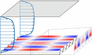
Figure 4 shows the solution $\bar {U}$ to (2.7a,b) for turbulent channel flow with $Re_\tau =186$ subject to a streamwise pressure gradient $\bar {P}_{x}=-1$ over triangular riblets. Here, $N_i=179, N_o=20, 25$ harmonics have been used to approximate the solution, i.e. $m = -12,\ldots ,12$, and the triangular riblets are characterized by $K^{-1}(y,z)$ with $h=0.0804, \omega _z=30, R = 1.5\times 10^5, s_f = 141$ and $r_p = 0.7434$. Figure 4 demonstrates that the solution respects the shape of riblets and is approximately zero in the solid region.

Figure 4. The streamwise mean velocity $\bar {U}(y,z)$ for turbulent channel flow with $Re_\tau =186$ over the triangular riblets given in figure 2(a).

2.3. Prediction of drag reduction

In what follows, subscripts $s$ and $c$ are used to signify channel flow with smooth walls and the correction that arises from surface corrugation. We use a variation in the driving pressure gradient to enforce a constant bulk flux requirement. This introduces a correction to the $0$th harmonic of the mean velocity as

(2.17)\begin{equation} \bar{U}_c(y) = \bar{U}_0(y) - (1 - \bar{P}_{x,c})\bar{U}_s(y). \end{equation}

Here, $\bar {U}_s(y)$ denotes the mean velocity profile in channel flow with smooth walls and the additional bulk introduced by the $0$th harmonic of the solution to (2.13) is used to compute the correction to pressure gradient $\bar {P}_{x,c}$, i.e.

(2.18)\begin{equation} \bar{P}_{x,c} = 1 - \frac{1}{U_B} \int_{-1-h r_p}^1\bar{U}_0(y) \, \mathrm{d} y. \end{equation}

The form of $\bar {P}_{x,c}$ ensures that the mean velocity correction $\bar {U}_{c}(y)$ in (2.17) has zero bulk. The corrections to the pressure gradient and mean velocity are used to compute the variation in skin-friction drag.

The rate of drag reduction caused by riblets is given by

(2.19)\begin{equation} {\rm \Delta} D \mathrel{\mathop:}= \left( D - D_s \right) /D_s, \end{equation}

where $D_s$ denotes the slope of the mean velocity at the lower wall in a flow without riblets. In a flow with riblets, the skin-friction drag at the lower wall can be computed using the pressure gradient, which maintains a constant bulk, and the well-defined slope of the mean velocity at the upper wall,

(2.20)\begin{equation} D = \bar{P}_{x} - \frac{\omega_z}{2{\rm \pi}} \int_0^{{2{\rm \pi}}/{\omega_z}} \frac{\partial {\bar{U}}}{\partial y}(y=1,z) \,\mathrm{d} z. \end{equation}

Since $\bar {P}_{x}=2D_s, {\rm \Delta} D$ is determined by the difference between the pressure gradient adjustment and the drag reduction at the upper wall, i.e.

(2.21)\begin{equation} {\rm \Delta} D = \frac{1}{D_s}\left[ \bar{P}_{x,c} - \left(\frac{\omega_z}{2{\rm \pi}} \int_0^{{2{\rm \pi}}/{\omega_z}} \frac{\partial \bar{U}}{\partial y}(y=1,z) \,\mathrm{d} z - D_s\right) \right]. \end{equation}

Even though the mean velocity profile shown in figure 4 respects the shape of riblets and goes to zero within the solid region, the resulting drag reduction does not follow trends reported in literature. As demonstrated in figure 5, the mean velocity profile resulting from the use of $\nu _{Ts}$ implies a reduction in drag regardless of the size of riblets. Furthermore, no optimal spacing that maximizes drag reduction is identified. To improve predictions of the mean velocity and the resulting skin-friction drag, in § 3 we extend the framework proposed in Moarref & Jovanovic (Reference Moarref and Jovanovic2012) to account for the effect of velocity fluctuations in a flow over riblets on the turbulent viscosity $\nu _T$.

Figure 5. Prediction of drag reduction in turbulent channel flow with $Re_\tau =186$ resulting from the steady-state solution of (2.7a,b) with $\nu _{Ts} (y)$ given by (2.11). Triangular riblets, shown in figure 7, with different peak-to-peak spacing but a constant height to spacing ratio $h/s = 0.38$ are considered and the spacing is reported in inner viscous units, i.e. $s^+ = Re_\tau s$.

3.1. Model equation for $\nu _T$

As described in § 2.3, $\nu _{Ts}$ does not provide the proper eddy viscosity model for channel flow with riblets. Establishing a relation between $\nu _T$ and the second-order statistics of velocity fluctuations represents the main challenge for identifying the appropriate eddy viscosity model. With appropriate choices of velocity and length scales, turbulent viscosity can be expressed as (Pope Reference Pope2000)

(3.1)\begin{equation} \nu_T(y) = c Re_\tau^2 \frac{k^2(y)}{\epsilon(y)}, \end{equation}

where $c = 0.09,$ $k$ is the turbulent kinetic energy and $\epsilon$ is the rate of dissipation. The $k$–${\epsilon }$ model (Jones & Launder Reference Jones and Launder1972; Launder & Sharma Reference Launder and Sharma1974) provides two differential transport equations for $k$ and ${\epsilon }$, but is computationally demanding and does not offer insight into analysis, design and optimization. On the other hand, wall-normal profiles for $k$ and ${\epsilon }$ can be obtained by averaging the second-order statistics of velocity fluctuations over the streamwise coordinate and one period of the spanwise surface corrugation:

(3.2a)\begin{gather} k(y) = \tfrac{1}{2} (\overline{\langle uu\rangle} + \overline{\langle vv\rangle} + \overline{\langle ww\rangle}) ,\\[-2.5pc]\nonumber\end{gather}

(3.2b)\begin{align} \epsilon(y) & = 2 (\overline{\langle u_xu_x\rangle} + \overline{\langle v_yv_y\rangle} + \overline{\langle w_zw_z\rangle} + \overline{\langle u_yv_x\rangle} + \overline{\langle u_zw_x\rangle} + \overline{\langle v_zw_y\rangle})\nonumber\\ & \quad + \overline{\langle u_yu_y\rangle} + \overline{\langle w_yw_y\rangle} + \overline{\langle v_xv_x\rangle} + \overline{\langle w_xw_x\rangle} + \overline{\langle u_zu_z\rangle} + \overline{\langle v_zv_z\rangle}. \end{align}

Here, overline denotes averaging in $x$ and one period in $z$. We next demonstrate how second-order statistics, e.g. $uu$, can be computed using the stochastically forced linearized NS equations.

3.2. Stochastically forced linearized Navier–Stokes equations

The dynamics of infinitesimal velocity ${\boldsymbol v}=[ u ~v ~w ]^\textrm {T}$ and pressure $p$ fluctuations around $\bar {{\boldsymbol u}} = [ {\bar {U}}(y,z) ~0 ~0 ]^\textrm {T}$ and $\bar {P}$ are governed by the linearized NS and continuity equations:

(3.3)\begin{gather} \partial_t {\boldsymbol v} = - ( \boldsymbol{\nabla} \boldsymbol{\cdot} \bar{{\boldsymbol u}} ) {\boldsymbol v} - ( \boldsymbol{\nabla} \boldsymbol{\cdot} {\boldsymbol v} ) \bar{{\boldsymbol u}} - \boldsymbol{\nabla} p - {K}^{-1}{\boldsymbol v} + \dfrac{1}{Re_\tau} \boldsymbol{\nabla}\boldsymbol{\cdot}((1 + \nu_T)( \boldsymbol{\nabla}{\boldsymbol v} + (\boldsymbol{\nabla}{\boldsymbol v})^\textrm{T} )) + \boldsymbol{f}, \end{gather}

(3.3)\begin{gather} 0 = \boldsymbol{\nabla} \boldsymbol{\cdot} {\boldsymbol v}. \end{gather}

Here $\boldsymbol {f}$ is a zero-mean white-in-time additive stochastic forcing. The normal modes in $x$ are given by $\textrm {e}^{\mathrm {i} k_x x}$, where $k_x$ is the streamwise wavenumber, and the normal modes in $z$ are given by the Bloch waves (Odeh & Keller Reference Odeh and Keller1964; Bensoussan, Lions & Papanicolaou Reference Bensoussan, Lions and Papanicolaou1978), which are determined by the product of $\textrm {e}^{\mathrm {i}\theta z}$ with $\theta \in [0,\omega _z/2)$ and a $2{\rm \pi} /\omega _z$ periodic function in $z$. For example, the forcing field in (3.3a,b) can be represented as

(3.4)\begin{equation} \left. \begin{array}{c@{}} \boldsymbol{f}(x,y,z,t) = \textrm{e}^{\mathrm{i} k_x x} \,\textrm{e}^{\mathrm{i}\theta z} \hat{\boldsymbol{f}}(k_x, y,z,t), \\ \hat{\boldsymbol{f}}(k_x,y,z,t) = \hat{\boldsymbol{f}}(k_x, y, z + 2{\rm \pi}/\omega_z, t), \end{array} \right\} \quad k_x \in \mathbb{R},\ \theta \in [0, \omega_z/2), \end{equation}

where real parts are used to represent physical quantities. The Fourier series expansion of the $2{\rm \pi} /\omega _z$-periodic function $\hat {\boldsymbol {f}}(k_x,y,z,t)$ can be used to obtain

(3.5)\begin{equation} \boldsymbol{f}(x,y,z,t) = \sum_{n \in \mathbb{Z}} \hat{\boldsymbol{f}}_n (k_x,y,\theta,t) \,\textrm{e}^{\mathrm{i}(k_x x + \theta_n z)}, \quad \begin{array}{l} \theta_n = \theta + n\omega_z,\\ k_x \in \mathbb{R},\ \theta \in [0, \omega_z/2), \end{array} \end{equation}

where $\{\,\hat {\boldsymbol {f}}_n (k_x,y,\theta ,t)\}_{n \in \mathbb {Z}}$ are the Fourier coefficients of the function $\hat {\boldsymbol {f}}(k_x,y,z,t)$ in (3.4).

Substituting (3.5) into the linearized equations (3.3a,b) and eliminating pressure through a standard conversion (Schmid & Henningson Reference Schmid and Henningson2001) yields the evolution form

(3.6a)\begin{gather} \partial_t \boldsymbol{\varphi}_\theta(k_x,y,t) = [\boldsymbol{A}_\theta(k_x) \boldsymbol{\varphi}_\theta (k_x, \cdot ,t)](y) + {\boldsymbol d}_\theta (k_x,y,t), \end{gather}

(3.6b)\begin{gather} {\boldsymbol v}_\theta(k_x,y,t) = [\boldsymbol{C}_\theta(k_x) \boldsymbol{\varphi}_\theta(k_x, \cdot ,t)](y), \end{gather}

with the state $\boldsymbol {\varphi }_\theta$ consisting of the wall-normal velocity $v$ and vorticity $\eta = \partial _z u - \partial _x w$. The state-space representation (3.6a,b) is parameterized by the streamwise wavenumber $k_x$ and the spanwise wavenumber offset $\theta$: for each $k_x$ and $\theta , \boldsymbol {\varphi }_\theta , {\boldsymbol v}_\theta$ and ${\boldsymbol d}_\theta \mathrel {\mathop :}= \boldsymbol {B}_\theta \boldsymbol {f}_{\theta }$ are bi-infinite column vectors, e.g. $\boldsymbol {\varphi }_{\theta }(k_x, y, t) = \text {col}\{ \hat {\boldsymbol {\varphi }}_n (k_x, y, \theta , t) \}_{n \in \mathbb {Z}}$, and $\boldsymbol {A}_{\theta }(k_x), \boldsymbol {B}_{\theta }(k_x)$, and $\boldsymbol {C}_{\theta }(k_x)$ are bi-infinite matrices whose elements are operators in $y$, e.g.

(3.7)\begin{equation} \boldsymbol{A}_\theta \mathrel{\mathop:}= \left[ \begin{array}{c@{}cccc@{}} \ddots & \vdots & \vdots & \vdots & {{{\mathinner{\mkern2mu\raise1pt\hbox{.}\mkern2mu \raise4pt\hbox{.}\mkern2mu\raise7pt\hbox{.}\mkern1mu}}}} \\ \cdots & \boldsymbol{A}_{n-1,0} & \boldsymbol{A}_{n-1,+1} & \boldsymbol{A}_{n-1,+2} & \cdots \\ \cdots & \boldsymbol{A}_{n,-1} & \boldsymbol{A}_{n,0} & \boldsymbol{A}_{n,+1} & \cdots \\ \cdots & \boldsymbol{A}_{n+1,-2} & \boldsymbol{A}_{n+1,-1} & \boldsymbol{A}_{n+1,0} & \cdots \\ {{\mathinner{\mkern2mu\raise1pt\hbox{.}\mkern2mu \raise4pt\hbox{.}\mkern2mu\raise7pt\hbox{.}\mkern1mu}}} & \vdots & \vdots & \vdots & \ddots \end{array} \right], \end{equation}

where the off-diagonal term $\boldsymbol {A}_{n,m}$ denotes the influence of the $(n+m)$th harmonic $\hat {\boldsymbol {\varphi }}_{n+m}$ on the dynamics of the $n$th harmonic $\hat {\boldsymbol {\varphi }}_{n}$. Apart from accounting for an extended wall-normal region, the block operators on the main diagonal of $\boldsymbol {A}_\theta$ are identical to the operators for the channel flow without riblets; see appendix A for details. At the upper wall of the channel, homogenous Dirichlet boundary conditions are imposed on $\eta$, and homogeneous Dirichlet and Neumann boundary conditions are imposed on $v$. Similar to the mean flow equations (2.7a,b), the boundary conditions at the corrugated surface are automatically satisfied via volume penalization. Finally, smoothness of all physical quantities at the intersection of the inner and outer wall-normal regimes ($y=-1$) is imposed by enforcing the following conditions:

\begin{gather} {v}(y = -1^+,z) = {v}(y = -1^-,z), \quad \frac{\partial v}{\partial y}(y=-1^+,z) = \frac{\partial v}{\partial y}(y=-1^-,z),\nonumber \end{gather}

\begin{gather}\frac{\partial ^2v}{\partial y^2}(y=-1^+,z) = \frac{\partial ^2v}{\partial y^2}(y=-1^-,z), \quad \frac{\partial ^3v}{\partial y^3}(y=-1^+,z) = \frac{\partial ^3v}{\partial y^3}(y=-1^-,z),\nonumber \end{gather}

\begin{gather}\eta(y=-1^+,z) = \eta(y=-1^-,z), \quad \frac{\partial \eta}{\partial y}(y=-1^+,z) = \frac{\partial \eta}{\partial y}(y=-1^-,z).\nonumber \end{gather}

A pseudospectral scheme used for discretizing the mean flow equations (2.7a,b) is utilized to discretize the wall-normal operators in (3.6a,b). In addition, a change of variables is employed to obtain a state-space representation in which the kinetic energy is determined by the Euclidean norm of the state vector in a finite-dimensional approximation of the evolution model (Zare et al. Reference Zare, Jovanovic and Georgiou2017b, appendix A),

(3.8a)\begin{gather} \dot{\boldsymbol{\psi}_\theta}(k_x,t) = A_\theta(k_x) \boldsymbol{\psi}_\theta (k_x,t) + {{\boldsymbol d}}_{\theta} (k_x,t), \end{gather}

(3.8b)\begin{gather} {\boldsymbol v}_\theta (k_x,t) = C_\theta (k_x) \boldsymbol{\psi}_\theta(k_x,t). \end{gather}

For $N_i$ and $N_o$ collocation points in the inner and outer wall-normal regimes, respectively, and a Fourier series expansion (2.8) with $M$ harmonics, $\boldsymbol {\psi }_\theta (k_x,t)$ and ${\boldsymbol v}_\theta (k_x,t)$ are vectors with $2\times M \times (N_i+N_o)$ and $3\times M \times (N_i+N_o)$ complex-valued entries, respectively. The state-space matrices $A_\theta (k_x)$ and $C_\theta (k_x)$ are discretized versions of the operators in (3.6a,b) that incorporate the aforementioned change of coordinates.

3.3. Second-order statistics of velocity fluctuations and forcing

Let the linearized dynamics (3.8a,b) be driven by zero-mean stochastic forcing $\boldsymbol {d}_\theta (k_x,t)$ that is white in time, with covariance matrix $M_\theta (k_x)=M^*_\theta (k_x) \succeq 0$, i.e.

(3.9)\begin{equation} \langle {\boldsymbol d}_\theta(k_x,t_1) {\boldsymbol d}^*_\theta(k_x,t_2) \rangle = M_\theta(k_x) \delta(t_1 - t_2), \end{equation}

where $\delta$ is the Dirac delta function. Following the bi-infinite structure of ${\boldsymbol d}_\theta (k_x,t), M_\theta (k_x)$ takes the bi-infinite form,

(3.10)\begin{equation} M_\theta(k_x) \mathrel{\mathop:}= \left[ \begin{array}{c@{}cccc@{}} \ddots & \vdots & \vdots & \vdots & {{\mathinner{\mkern2mu\raise1pt\hbox{.}\mkern2mu \raise4pt\hbox{.}\mkern2mu\raise7pt\hbox{.}\mkern1mu}}} \\ \cdots & M(k_x, \theta_{n-1}) & 0 & 0 & \cdots \\ \cdots & 0 & M(k_x, \theta_{n}) & 0 & \cdots \\ \cdots & 0 & 0 & M(k_x, \theta_{n+1}) & \cdots \\ {{\mathinner{\mkern2mu\raise1pt\hbox{.}\mkern2mu \raise4pt\hbox{.}\mkern2mu\raise7pt\hbox{.}\mkern1mu}}} & \vdots & \vdots & \vdots & \ddots \end{array} \right], \end{equation}

with the block operator $M(k_x, \theta _{n})$ representing the covariance of the $n$th harmonic of the forcing ${\boldsymbol d}_\theta (k_x,t)$. The off-diagonal blocks of $M_\theta (k_x)$ are zero because the stochastic forcing is uncorrelated over various spanwise harmonics.

The steady-state covariance of the state in (3.8a,b) can be determined from the solution $X_\theta (k_x)$ to the Lyapunov equation (Fardad, Jovanovic & Bamieh Reference Fardad, Jovanovic and Bamieh2008; Moarref & Jovanovic Reference Moarref and Jovanovic2010)

(3.11)\begin{equation} A_\theta(k_x) {X}_\theta(k_x) + {X}_\theta(k_x) A_\theta^*(k_x) = -M_\theta(k_x), \end{equation}

where the ($i,j$)th block of ${X}_\theta (k_x)$ determines the correlation matrix associated with the $i$th and $j$th harmonics of the state $\boldsymbol {\psi }_\theta$.

As mentioned in § 3.2, the block operators on the main diagonal of $A_\theta$ contain the dynamical generators of the turbulent channel flow with smooth walls at various wavenumber pairs $(k_x,\theta _n)$. Based on this, $A_\theta$ can be decomposed as

(3.12)\begin{equation} A_\theta(k_x) = A_{\theta, s}(k_x) + A_{\theta, c}(k_x), \end{equation}

where $A_{\theta , s} = {\mathrm {diag}}\{ \ldots , A_s(k_x,\theta _{n-1}), A_s(k_x,\theta _n), A_s(k_x,\theta _{n+1}), \ldots \}$ accounts for the dynamical generator of the turbulent channel flow with smooth walls and $A_{\theta , c}$ captures the contribution of the spatially periodic surface corrugation. The block-diagonal structure of $M_\theta (k_x)$ implies that the solution $X_\theta (k_x)$ to (3.11) can also be decomposed as

(3.13)\begin{equation} X_\theta(k_x) = X_{\theta, s}(k_x) + X_{\theta, c}(k_x). \end{equation}

Here, $X_{\theta , s} = {\mathrm {diag}}\{ \ldots , X_s(k_x,\theta _{n-1}), X_s(k_x,\theta _n), X_s(k_x,\theta _{n+1}), \ldots \}$ is a block-diagonal covariance operator whose entries are determined by the steady-state covariance matrix of turbulent channel flow over smooth walls parameterized by $(k_x,\theta _n)$, and $X_{\theta , c}$ denotes the modification resulting from the presence of riblets. This follows from substitution of (3.12) and (3.13) into the Lyapunov equation (3.11),

(3.14)\begin{align} &(A_{\theta,s}(k_x) + A_{\theta, c}(k_x))(X_{\theta,s}(k_x) + X_{\theta, c}(k_x)) \nonumber\\ &\quad +(X_{\theta,s}(k_x) + X_{\theta, c}(k_x))(A_{\theta,s}(k_x) + A_{\theta, c}(k_x))^* =-M_\theta(k_x), \end{align}

from which the Lyapunov equation corresponding to the turbulent channel flow with smooth walls can be extracted as

(3.15)\begin{equation} A_{\theta, s}(k_x) X_{\theta,s} (k_x) + X_{\theta, s}(k_x) A_{\theta,s}(k_x) = -M_\theta(k_x). \end{equation}

Following Moarref & Jovanovic (Reference Moarref and Jovanovic2012), we select the block-diagonal covariance matrix $M_\theta (k_x)$ to guarantee equivalence between the two-dimensional energy spectrum of the turbulent channel flow with smooth walls and the flow governed by the stochastically forced NS equations linearized around $\bar {{\boldsymbol u}}=[ {\bar {U}_s}(y)~ 0~ 0 ]^\textrm {T}$. This is achieved by scaling the block covariances in (3.10) as

(3.19a)\begin{equation} M(k_x,\theta_{n}) = \frac{\bar{E}_s(k_x, \theta_{n})}{\bar{E}_{s,0}(k_x, \theta_{n})} M_s(k_x, \theta_{n}).\nonumber \end{equation}

Here, $\bar {E}_s(k_x,\theta _{n}) = \int _{-1}^{1} E_s(y, k_x, \theta _{n}) \,\mathrm {d} y$ is the two-dimensional energy spectrum of a turbulent channel flow with smooth walls, which is obtained from the DNS-based energy spectrum $E_s(y, k_x, \theta _{n})$ (Del Álamo & Jiménez Reference Del Álamo and Jiménez2003; Del Álamo et al. Reference Del Álamo, Jiménez, Zandonade and Moser2004), and $\bar {E}_{s,0}(k_x, \theta _{n})$ is the energy spectrum resulting from the linearized NS equations (3.8a,b) subject to white-in-time stochastic forcing with the covariance matrix

(3.16)\begin{align} M_s(k_x, \theta_{n}) = \left[ \begin{matrix} \sqrt{E_s(y,k_x,\theta_{n})} I & 0 \\ 0 & \sqrt{E_s(y,k_x,\theta_{n})} I \end{matrix} \right] \left[ \begin{matrix} \sqrt{E_s(y,k_x,\theta_{n})} I & 0 \\ 0 & \sqrt{E_s(y,k_x,\theta_{n})} I \end{matrix} \right] ^*. \end{align}

Finally, the energy spectrum of velocity fluctuations is determined from the solution to the Lyapunov equation (3.11) as

(3.17)\begin{equation} {\bar{E}(k_x,\theta) = \sum_{n \in \mathbb{Z}} {\mathrm{trace}} (X_d(k_x,\theta_n) ),} \end{equation}

where $X_d(k_x,\theta _n)$ represent the block covariance matrices on the main diagonal of $X_\theta (k_x)$ confined to the wall-normal range of $y\in [-1, 1]$. The correction to the energy spectrum that arises from the presence of riblets is determined by

(3.18)\begin{equation} \bar{E}_c(k_x,\theta) = \bar{E}(k_x,\theta) - \bar{E}_s(k_x,\theta), \end{equation}

where

(3.19)\begin{equation} \bar{E}_s(k_x,\theta) = \sum_{n \in \mathbb{Z}} \bar{E}_s(k_x,\theta_{n}) \end{equation}

denotes the reference energy spectrum from DNS of channel flow in the absence of riblets.

3.4. Correction to turbulent viscosity

The turbulent viscosity $\nu _T(y)$ is determined by the second-order statistics of velocity fluctuations, i.e. the kinetic energy $k(y)$ and its rate of dissipation ${\epsilon }(y)$; see (3.1). The statistics can be computed using the covariance matrix $X_d(k_x,\theta _n)$ and $k(y), {\epsilon }(y)$ can be decomposed as

(3.20a,b)\begin{equation} k(y) = k_s(y) + k_c(y), \quad \epsilon(y) = \epsilon_s(y) + \epsilon_c(y), \end{equation}

where, again, the subscript $s$ signifies channel flow with smooth walls and the subscript $c$ quantifies the influence of fluctuations in the flow over riblets. The DNS results for turbulent channel flow yield $k_s$. On the other hand, ${\epsilon }_s$ is computed using ${\epsilon }_s (y) = c Re_\tau ^2 k_s^2 (y)/\nu _{Ts} (y)$ and the corrections $k_c$ and $\epsilon _c$ can be determined from the second-order statistics in $X_{\theta ,c}(k_x)$; see appendix B for details. Substitution of $k(y)$ and ${\epsilon }(y)$ from (3.20a,b) into (3.1) and application of the Neumann series expansion yields

(3.21)\begin{equation} \nu_T(y) = \nu_{Ts}(y) + \nu_{Tc}(y), \end{equation}

where the correction $\nu _{Tc}(y)$ to turbulent viscosity $\nu _{Ts}(y)$ is given by

(3.22)\begin{equation} \nu_{Tc}(y) = \nu_{Ts}(y) \left(\frac{2 k_c(y)}{k_s(y)} - \frac{\epsilon_c(y)}{\epsilon_s(y)}\right). \end{equation}

Since we primarily focus on small-size riblets, this expression is obtained by neglecting higher-order terms that involve multiplication of $k_c(y)$ and ${\epsilon }_c(y)$.

The influence of fluctuations on the turbulent mean velocity and, consequently, skin-friction drag can be evaluated by substituting $\nu _T(y)$ from (3.21) and solving equations (2.7a,b); see § 2.2 for details regarding the correction to the mean flow profile and § 2.3 for the subsequent computation of the drag.

4.1. Drag reduction

We first examine the effect of riblet size on turbulent drag. In our parametric study, we follow García-Mayoral & Jiménez (Reference García-Mayoral and Jiménez2011b) and refer to the regime of vanishing riblet spacing, in which the drag reduction is proportional to the size of riblets, as the viscous regime. For turbulent channel flow with $Re_\tau =186$ subject to triangular riblets on the lower wall, figure 8 shows the influence of the height and peak-to-peak spacing of riblets on ${\rm \Delta} D$ in (2.21). In this figure the height and spacing are reported in inner viscous units, i.e. $h^+ = Re_\tau h$ and $s^+ = Re_\tau s$, and various curves represent different tip angles $\alpha$ as a measure of riblet geometry. As shown in figure 7, a particular tip angle $\alpha$ corresponds to a specific height to spacing ratio.

Figure 8. Turbulent drag reduction for triangular riblets with different tip angles $\alpha$ as a function of (a) spacing $s^+$; and (b) height $h^+$ in a channel flow with $Re_\tau =186$ and $\alpha =105^\circ$ ($\raisebox{6pt}{\rotatebox{180}{$\triangle$}}$); $90^\circ$ ($\triangle$); $75^\circ$ ($\raisebox{2pt}{{$_\ocircle$}}$); $60^\circ$ ($\lozenge$); and $45^\circ$ ($\times$), as well as $Re_\tau =547$ and $\alpha =90^\circ$ ($\square$).

Clearly, small-size riblets can indeed reduce skin-friction drag. Figure 8 shows the percentage of drag reduction obtained in turbulent channel flows with $Re_\tau =186$ and $Re_\tau =547$ over the different triangular riblets listed in table 1. Herein, we focus on the channel flow with $Re_\tau =186$ to analyse the dependence of drag reduction on the spacing and height of riblets. Figure 8(a) demonstrates that, for $s^+<20$, the drag reduction first increases as $h^+$ increases, saturates and then decreases. This trend, however, slows down for smaller values of $s^+$. For $\alpha =90^\circ$ and $\alpha =60^\circ$, the drag-reduction trends and optimal $s^+$ values resulting from our method reliably capture the trends reported in experimental studies (Bechert et al. Reference Bechert, Bruse, Hage, Van der Hoeven and Hoppe1997). On the other hand, as shown in figure 8(b), for a fixed height, as the spacing $s^+$ of riblets decreases, drag reduction increases, saturates and then decreases. Furthermore, figures 8(a) and 8(b) show that as the riblet tip angle $\alpha$ decreases, maximum drag reduction is achieved for less separated and taller riblets, respectively. Finally, as $\alpha$ decreases, the maximum value of drag reduction first increases and then decreases, which is also in agreement with experimental observations (Bechert et al. Reference Bechert, Bruse, Hage, Van der Hoeven and Hoppe1997). The trends predicted by our framework indicate an optimal height to spacing ratio of $h/s\approx 0.65$ $(\alpha =75^\circ )$ for triangular riblets, which overpredicts the previously reported optimal tip angle $\alpha =54^\circ$ (Dean & Bhushan Reference Dean and Bhushan2010).

As demonstrated in figure 8, the optimal height and spacing can be quite different for riblets of different shape (i.e. different values of $\alpha$), thereby indicating that the height and spacing may not be suitable metrics for characterizing the breakdown of the linear viscous regime. Instead, the groove cross-section area $l_g^+ \mathrel {\mathop :}=\sqrt {A^+}$ (for triangular riblets, $A^+ = h^+s^+/2$) provides the best collapse of the critical breakdown dimension across different riblet shapes (García-Mayoral & Jiménez Reference García-Mayoral and Jiménez2011a,Reference García-Mayoral and Jiménezb). Furthermore, to remove the effect of riblets’ shape on their slope in the viscous regime $m_l \mathrel {\mathop :}= \lim _{l_g^+ \rightarrow 0}{{\rm \Delta} D}/{l_g^+}$, we normalize the drag-reduction curves by $m_l$ (García-Mayoral & Jiménez Reference García-Mayoral and Jiménez2011b).

For turbulent channel flow over triangular riblets, figure 9 shows the $m_l$-normalized drag reduction as a function of $l_g^+$. The normalization factor $m_l$ is computed by averaging the slope obtained from the first two points on each curve, which are both in the viscous regime. The shaded region represents the envelope of normalized drag-reduction values resulting from prior experimental and numerical studies (García-Mayoral & Jiménez Reference García-Mayoral and Jiménez2011b). For riblets with $\alpha = 105^\circ , 90^\circ , 75^\circ , 60^\circ$ and $45^\circ$, figure 9 shows the collapse of drag-reduction curves with the largest drag reduction occurring within a tight range of cross-section areas; $l_g^+=9.7, 11.1, 11.3, 11.3$ and $10.2$ for $\alpha = 105^\circ , 90^\circ , 75^\circ , 60^\circ$ and $45^\circ$, respectively. This prediction agrees well with the values reported by García-Mayoral & Jiménez (Reference García-Mayoral and Jiménez2011b), $l_g^+ \in [ 9.7, 11.7]$. Moreover, the drag-reduction curves resulting from our framework are located within the shaded region and they reliably predict the overall trend. For turbulent channel flow over triangular riblets with $Re_\tau =547, h/s=0.5$ and $\alpha = 90^\circ$, our predictions of the normalized drag reduction remain within this shaded region and are very similar to the results obtained for $Re_\tau =186$; see square symbols in figure 9.

Figure 9. Drag reduction normalized with its slope in the viscous regime $m_l$. Different shapes of triangular riblets are represented by $\alpha =105^\circ$ ($\raisebox{6pt}{\rotatebox{180}{$\triangle$}}$); $90^\circ$ ($\triangle$); $75^\circ$ ($\raisebox{2pt}{{$_\ocircle$}}$); $60^\circ$ ($\lozenge$); $45^\circ$ ($\times$) for $Re_\tau =186$; and $\alpha = 90^\circ$ ($\square$) for $Re_\tau =547$. The shaded area shows the envelope of experimental and numerical results (Bechert et al. Reference Bechert, Bruse, Hage, Van der Hoeven and Hoppe1997; García-Mayoral & Jiménez Reference García-Mayoral and Jiménez2011b).

Figure 10 compares the $m_l$-normalized drag reduction resulting from our framework and the experimental results of Bechert et al. (Reference Bechert, Bruse, Hage, Van der Hoeven and Hoppe1997). Our method captures the overall trends and even the optimal size of riblets with tip angle $\alpha =60^\circ$ ($2.9\,\%$ relative error). For riblets with tip angle $\alpha =90^\circ$, the optimal size is overpredicted by $14.3\,\%$. We note that while the maximum amount of drag reduction is reasonably captured in both cases ($13.1\,\%$ and $7.6\,\%$ relative errors for $\alpha =60^\circ$ and $\alpha =90^\circ$, respectively), the quality of our predictions deteriorates for larger riblets with $\alpha =90^\circ$. As we discuss in § 4.2, an overpredicted turbulence suppression in wall-normal regions away from the riblet-mounted lower surface can be a source of this mismatch.

Figure 10. Drag reduction normalized with its slope in the viscous regime $m_l$ resulting from our framework (open symbols) and experiments (solid symbols) (Bechert et al. Reference Bechert, Bruse, Hage, Van der Hoeven and Hoppe1997) with tip angles (a) $\alpha = 60^\circ$; and (b) $90^\circ$ for $Re_\tau =186$.

The performance deterioration for large riblets observed in figures 9 and 10 is associated with the breakdown of the viscous regime within the grooves. This breakdown arises from the lodging of near-wall vortices (Suzuki & Kasagi Reference Suzuki and Kasagi1994; Lee & Lee Reference Lee and Lee2001), the generation of secondary flow vortices (Goldstein & Tuan Reference Goldstein and Tuan1998) or the emergence of spanwise coherent rollers (García-Mayoral & Jiménez Reference García-Mayoral and Jiménez2011b). When turbulence moves into the grooves, a turbulence model, which assumes that the wall-normal region with $y<-1$ is laminar (i.e. $\nu _T=0$), loses its validity. To support an extended turbulent regime and go beyond the breakdown of the viscous regime, our model of surface corrugation assumes the tip of riblets to be located within the original channel region (i.e. $y>-1$); see § 2.1. The parameter $r_p$ in (2.10), which controls the level of protrusion into the turbulent regime, is determined to satisfy a constant bulk assumption. Because of this, our model remains valid even for riblets that are larger than the optimal ($l_g^+\lesssim 20$).

4.2. Effect of riblets on turbulent viscosity and turbulent mean velocity

We next examine the effect of riblets on turbulent viscosity and mean velocity. Figure 11 shows the turbulent eddy viscosity $\nu _{Ts}$ and mean velocity $\bar {U}_s$ of channel flow over smooth walls with $Re_\tau =186$ along with the corresponding corrections, $\nu _{Tc}$ and $\bar {U}_c$, introduced by riblets with $\alpha =90^\circ$ on the lower wall. The wall-normal coordinate is given in inner (viscous) units, i.e. $y^+=Re_\tau (1+y)$. Among the cases listed in table 1, cases with maximum drag reduction $(\omega _z=50)$, minimum drag reduction $(\omega _z=30)$ and smallest riblets $(\omega _z=160)$ are chosen. For $\omega _z=30$, figure 11(c) shows that turbulence is promoted at the beginning of the buffer layer, but is then suppressed in regions farther away from the wall. On the other hand, for $\omega _z=50$, turbulence is always suppressed ($\nu _{Tc} \leq 0$) and the region of suppression shifts closer to the wall ($y^+ \gtrsim 3$). We observe similar trends for riblets with $\omega _z=160$ to riblets with $\omega _z=50$, but with smaller amplitude. Figure 11(d) shows that, in all cases, riblets reduce the mean velocity gradient in the immediate vicinity of the wall ($y^+ \lesssim 6$). These results demonstrate that for the same shape of riblets (i.e. same tip angle $\alpha$), riblets of sizes that are larger than the optimal yield smaller amounts of turbulence suppression and mean shear reduction.

Figure 11. (a) The turbulent viscosity, $\nu _{Ts}(y^+)$; and (b) the turbulent mean velocity ${\bar {U}_s}(y^+)$ in an uncontrolled channel flow with $Re_\tau =186$. The correction to (c) turbulent viscosity, $\nu _{Tc}(y^+)$; and (d) the mean velocity, $\bar {U}_c(y^+)$, in the presence of riblets with $\alpha =90^\circ$. Red solid lines correspond to riblets with $\omega _z=30$ (minimum drag reduction), blue dashed lines correspond to riblets with $\omega _z=50$ (maximum drag reduction) and black dotted lines correspond to riblets with $\omega _z=160$ (smallest riblets).

To illustrate the influence of the shape of riblets on turbulent viscosity and mean velocity, figure 12 shows $\nu _{Tc}$ and $\bar {U}_c$ for turbulent channel flow over riblets with different tip angles $\alpha$ and with spanwise frequencies $\omega _z$ that correspond to the maximum drag reduction. The largest turbulence suppression and mean velocity reduction is achieved for $\alpha =75^\circ$, which is in agreement with the drag-reduction trends observed in figure 8. Between $\alpha =45^\circ$ and $\alpha =105^\circ$, the reduction in turbulent viscosity is more pronounced for the latter, which again reflects the drag-reduction trends reported in figure 8.

Figure 12. Correction to (a) turbulent viscosity $\nu _{Tc}(y^+)$; and (b) mean velocity $\bar {U}_c(y^+)$ in turbulent channel flow with $Re_\tau =186$ over triangular riblets on the lower wall. The spanwise frequency $\omega _z$ associated with different shapes is selected to maximize drag reduction: $\alpha =105^\circ , \omega _z=50$ (solid black); $\alpha =75^\circ$; $\omega _z=60$ (dotted red); $\alpha =45^\circ , \omega _z=100$ (dot–dashed blue).

For riblets with $\alpha =60^\circ$ and $\omega _z=60$ ($s^+\approx 20$), figure 13 shows the variation of the mean velocity in the spanwise plane. No variation is found above $y>-0.9$, which is in agreement with the result of numerical simulations (Choi et al. Reference Choi, Moin and Kim1993). However, our predictions of the mean velocity profiles deviate from the result of DNS in the vicinity of the wall. This is because we have set the location of riblets to be slightly lower than the DNS computations in order to satisfy the constant bulk criteria. On the other hand, our results show a consistent promotion in the lower half and suppression in the upper half of the channel resulting in a slight lack of symmetry with respect to the centreline. This is mainly because of an overpredicted correction to turbulent eddy viscosity $\nu _{Tc}$ in the buffer layer and the inertial sublayer; cf. figure 11(c). Such overpredicted levels of turbulence suppression and drag reduction (cf. figures 8 and 10b) are caused by high amplitude stochastic forcing to the linearized equations (3.8a,b), which is shaped to match the two-dimensional DNS energy spectrum (§ 3.3). Analysing the efficacy of more sophisticated forcing schemes (Zare, Jovanovic & Georgiou Reference Zare, Jovanovic and Georgiou2016; Zare et al. Reference Zare, Chen, Jovanovic and Georgiou2017a,Reference Zare, Jovanovic and Georgioub) that may refine mean velocity predictions is a topic for future research.

Figure 13. Mean velocity profiles $\bar {U}(y,z)$ normalized with the laminar centreline velocity $U_l$ for $\alpha =60^\circ$ and $\omega _z=60$ ($s^+\approx 20$): (a) One-dimensional view for different spanwise locations ($z\in [0,{\rm \pi} /60]$) from our model (black curves) and the profile corresponding to $z\approx {\rm \pi}/120$ resulting from DNS of Choi et al. (Reference Choi, Moin and Kim1993) (blue circles). The direction of the arrow points to velocity profiles corresponding to spanwise locations farther away from the tip of riblets. (b) Colour plot of the streamwise mean velocity in the cross-plane.

4.3. Effect of riblets on turbulent kinetic energy

We next examine the effect of triangular riblets on the fluctuations’ kinetic energy. Figure 14 compares the reference energy spectrum of turbulent channel flow with smooth walls ((3.19)) to the changes in the energy spectrum caused by equally shaped riblets of different sizes ($\omega _z = 160, 50$ and $30$) with $\alpha =90^\circ$ ((3.18)). The energy spectra are premultiplied by the logarithmically scaled streamwise wavenumber $k_x$ so that the areas under the plots determine the total kinetic energy. Since the spanwise direction involves the parameterization $\theta _n = \theta + n \omega _z$, summation over $n$ is performed to integrate the energetic contribution of various harmonics in $\omega _z$ and identify the dependence of the energy spectrum on $\theta$; see § 3.3.

Figure 14. The premultiplied reference energy spectrum $k_x {\bar {E}_s}(k_x,\theta )$ ((3.19)) from DNS of turbulent channel flow with $Re_\tau =186$ (Del Álamo & Jiménez Reference Del Álamo and Jiménez2003) (left column), and the correction to the premultiplied spectrum $k_x {\bar {E}_c}(k_x,\theta )$ ((3.18)) due to the presence of various sizes of triangular riblets with $\alpha =90^\circ$ (right column): (a,b) $\omega _z=160$ ($l_g^+=3.6$); (c,d) $\omega _z=50$ ($l_g^+=11.7$, optimal); and (e,f) $\omega _z=30$ ($l_g^+=19.5$).

For channel flow over smooth walls with $Re_\tau =186$, the colour plots in the left column of figure 14 show that the most energetic modes take place at $(k_x,\theta )=(2.5,3.5)$. As blue regions in figures 14(b), 14(d) and 14(f) illustrate, riblets reduce the energy content of flow structures with smaller streamwise wavenumbers. Moreover, the yellow and red regions in figures 14(d) and 14(b) demonstrate that larger riblets increase the energy content of flow structures with larger streamwise wavenumbers. For these three cases, the largest energy amplification takes place around $(k_x,\theta )=(5.5,2.4), (6.4,4.6)$ and $(6.4,0.6)$, respectively. On the other hand, the maximum energy reduction occurs around $(k_x,\theta )=(4.9,0.9), (4.0,0.5)$ and $(4.0,0.5)$, respectively. Although the peak points are different, figures 14(b), 14(d) and 14(f) demonstrate similar amplification/suppression trends: riblets suppress/increase energy content of long/short streamwise length scales. These results provide evidence that the analysis of spatially periodic systems, e.g. the one considered in this paper, cannot be limited to a single horizontal wavenumber pair associated with the peak of the energy spectrum or the dominant near-wall cycle. We note that similar conclusions were reached in the analysis of turbulent channel flow subject to transverse wall oscillations (Moarref & Jovanovic Reference Moarref and Jovanovic2012). Finally, the dependence of correction ${\bar {E}_c}(k_x,\theta )$ on the shape of riblets is shown in figure 15. For all cases shown in this figure, similar modes are affected by the presence of riblets and the suppression of kinetic energy is more pronounced for riblets with $\alpha =75^\circ$ and $\omega _z=60$, which also yield the largest drag reduction (cf. figure 8). This suggests a synchrony between the dependence of drag reduction and energy suppression on the geometry of triangular riblets.

Figure 15. Correction to the premultiplied energy spectrum $k_x \bar {E}_c(k_x,\theta )$ in turbulent channel flow with $Re_\tau =186$ over triangular riblets of different size. The spanwise frequency $\omega _z$ associated with different shapes of riblets corresponds to maximum drag reduction: (a) $\alpha =105^\circ$, $\omega _z=50$; (b) $\alpha =75^\circ , \omega _z=60$; and (c) $\alpha =45^\circ$, $\omega _z=100$.

Figure 16(a) shows the percentage of kinetic energy variation ${\rm \Delta} E \mathrel {\mathop :}= \hat {E}_c/\hat {E}_s$ for triangular riblets as a function of the riblet groove area $l_g^+$. Here, $\hat {E}_c$ and $\hat {E}_s$ denote the correction to kinetic energy due to the presence of riblets and the kinetic energy of velocity fluctuations in the absence of riblets, respectively. These two quantities can be computed by integrating the corresponding energy spectra, i.e. $\bar {E}_c(k_x,\theta )$ and $\bar {E}_s(k_x,\theta )$, over all horizontal wavenumbers $k_x$ and $\theta$. On the other hand, figure 16(b) shows the percentage of drag reduction for the same values of $l_g^+$. Our computations demonstrate similar trends in the dependence of ${\rm \Delta} {E}$ and ${\rm \Delta} D$ on $l_g^+$ (cf. figure 16a,b), especially for the riblets in the viscous regime. Based on the various cases considered in figure 16, the linear regression model ${\rm \Delta} D = 1.7152 {{\rm \Delta} {E}} + 1.0907$ can be extracted with a coefficient of determination $R^2=0.9925$ for riblets with $l_g^+ \leq 14$. A strong correlation between changes in turbulent drag and kinetic energy suggests that energy can be used as a surrogate for predicting the effect of riblets on skin-friction drag; see figure 17(a). We note that a similar linear relation (but with a different slope) can be observed at $Re_\tau =547$. These results are not reported here for brevity.

Figure 16. (a) Kinetic energy suppression; and (b) turbulent drag reduction in channel flow with $Re_\tau =186$ over triangular riblets of different size. Symbols denote different shapes of triangular riblets with $\alpha =105^\circ$ ($\raisebox{6pt}{\rotatebox{180}{$\triangle$}}$); $90^\circ$ ($\triangle$); $75^\circ$ ($\raisebox{2pt}{{$_\ocircle$}}$); $60^\circ$ ($\lozenge$); and $45^\circ$ ($\times$).

Figure 17. (a) A linear relation between the turbulent drag reduction ${\rm \Delta} D$ and the kinetic energy suppression ${\rm \Delta} E$ for channel flow with $Re_\tau =186$ over triangular riblets of different size $l_g^+$. Circles mark cases listed in table 1 and crosses mark data for riblets with $l_g^+ \leq 14$. The red line provides a linear regression for the crosses. (b) The coefficient of determination $R^2$ for linear regression models resulting from data with $l_g^+\leq l_{g_T}^+$.

As shown in figure 11(c), riblets can suppress or enhance turbulence near the wall. Small riblets can disturb the near-wall cycle in the turbulent flow by generating and preserving laminar regions within the grooves. On the other hand, for larger riblets, streamwise rollers penetrate into the grooves which enhances turbulence close to the wall. As a result, nonlinear effects take over and the linear relation between drag/energy reduction and any metric of the riblet size (e.g. $l_g$) becomes compromised. As illustrated in figure 17(b), the quality of a linear regression model drops (i.e. $R^2$ becomes smaller) when data for larger-size riblets is taken into account.

5.1. Near-wall cycle in turbulent channel flow with $Re_\tau =186$

In the absence of riblets, the so-called near-wall cycle dominates the physics of the turbulent channel flow by generating streamwise streaks from the advection of the mean shear by streamwise vortices and the formation of streamwise vortices through streak instability and nonlinear interactions (Robinson Reference Robinson1991; Hamilton, Kim & Waleffe Reference Hamilton, Kim and Waleffe1995; Jiménez & Pinelli Reference Jiménez and Pinelli1999). Riblets can break this near-wall cycle and push the streamwise vortices and streaks away from the wall so that a laminar region is retained within the grooves. This ultimately reduces skin-friction drag. The typical wavelength of the flow structures in the near-wall cycle are reported as $(\lambda _x^+, \lambda _z^+) \approx (1000,100)$, which corresponds to $(k_x,\theta ) \approx (1.1687,11.687)$ in turbulent channel flow with $Re_\tau =186$.

For different sizes of riblets, figure 18 compares the flow structures that correspond to the near-wall cycle in turbulent channel flow with $Re_\tau =186$. Flow patterns resulting from the combination of streaks and vortices can be clearly observed. In particular, it is evident that the quasi-streamwise vortices and regions of high and low streamwise velocity are pushed above the riblet tips creating a region of limited turbulence in the riblet grooves, and effectively impeding the transfer of mean momentum toward the lower wall. The first two rows of figure 18 illustrate the flow structures over small- and optimal-sized riblets, respectively. The dominance of streamwise elongated structures that follow the length scales of the near-wall cycle is evident in these two scenarios. However, as shown in figure 18(e,f), the flow over larger riblets is contaminated by multiple energetically relevant spanwise length scales. This indicates an energy distribution across multiple Fourier modes beyond the ones that are relevant in the near-wall cycle. This distribution of energy is caused by the interaction of near-wall turbulence with the spanwise-periodic surface, which leads to the generation of secondary flow structures that follow the spatial frequency of riblets close to their tips (Goldstein & Tuan Reference Goldstein and Tuan1998); see figure 18(f).

Figure 18. Dominant flow structures in the vicinity of the lower wall of turbulent channel flow with $Re_\tau =186$ over triangular riblets with $\alpha =90^\circ$ and (a,b) $\omega _z = 160$; (c,d) $\omega _z = 50$; and (e,\,f) $\omega _z = 30$. These flow structures correspond to $(\lambda _x^+, \lambda _z^+) = (1000,100)$, typical scales of the near-wall cycle, and are extracted from the dominant eigenmode pair of the covariance matrix $\varPhi _\theta (k_x)$. Left column: $x-z$ slice of the streamwise velocity $u$ at $y^+ \approx 6$; Right column: $y-z$ slice of $u$ along with the vector field $(v, w)$ at $x^+ = 500$, which corresponds to the thick black lines in the left column. Colour plots are used for the streamwise velocity fluctuation $u$ and vector fields identify streamwise vortices.

The cross-plane views in figure 18 also show that, for larger riblets, secondary flow structures begin to penetrate into the grooves. This induces high-momentum flow into the viscous flow regime, which is reflected by an increase in the amplitude of velocity fluctuations at $y^+ \approx 6$ and the breakdown stage of the viscous regime which precedes the deterioration of drag reduction. Moreover, the kinetic energy corresponding to the length scale of the near-wall cycle varies from $0.0498$ for a channel flow with smooth walls, to $0.0468, 0.0441$ and $0.0609$ (given by $\bar {E}(k_x,\theta )$ defined in (3.17)) for small, optimal and large riblets, respectively. This shows that small- and optimally-sized riblets suppress the energy of near-wall cycle flow structures while larger ones can promote their energy, which is consistent with the trend observed in § 4.3.

5.2. Spanwise rollers resembling Kelvin–Helmholtz vortices

In addition to the influence of secondary flow structures around the tip of riblets, the breakdown of the viscous regime and decrease in drag reduction can also result from the amplification of spanwise rollers that are induced by a two-dimensional K–H instability (García-Mayoral & Jiménez Reference García-Mayoral and Jiménez2011b). The amplification of long spanwise scales for large riblets is evident from the energy spectra shown in figure 14. Figure 19 shows the DNS-based premultiplied streamwise co-spectra of various Reynolds stresses for infinitely wide scales ($\theta = 0$) in turbulent channel flow with $Re_\tau =186$ (Del Álamo & Jiménez Reference Del Álamo and Jiménez2003; Del Álamo et al. Reference Del Álamo, Jiménez, Zandonade and Moser2004), as well as the corresponding co-spectra resulting from our analysis of the flow over triangular riblets of different size. For larger riblets, the amplification of the co-spectra corresponding to streamwise and wall-normal intensities become stronger and occur closer to the wall. However, this trend is not observed for the co-spectrum corresponding to the spanwise turbulence intensity, which shows smaller amplification of channel-wide scales for riblets of larger size. Nevertheless, as the size of riblets increases, the co-spectrum corresponding to the wall-shear stress, $-k_xE_{uv}$, starts to show signs of suppression in the vicinity of the wall; the penetration of negative shear stress into the riblet grooves is evident from the co-spectrum associated with spatial frequency $\omega _z=30$. The co-spectrum $-k_xE_{uv}$ shows the largest suppression of shear stress for streamwise wavelengths $\lambda _x^+\approx 200$. Our results demonstrate that large riblets result in the suppression of shear stress within the grooves, which is consistent with our earlier findings that showed a degradation of drag reduction for such sizes (cf. figure 9). We note that our computations illustrate that the trends observed for the energy spectra do not vary for different shapes of riblets (i.e. different values of $\alpha$).

Figure 19. Premultiplied streamwise co-spectra at $\theta =0$ for turbulent channel flow with $Re_\tau =186$ over triangular riblets of tip angle $\alpha =90^\circ$. The four rows correspond to $k_xE_{uu}$, $k_xE_{vv}$, $k_xE_{ww}$ and $-k_xE_{uv}$; the four columns represent DNS data for the uncontrolled channel flow (Del Álamo & Jiménez Reference Del Álamo and Jiménez2003; Del Álamo et al. Reference Del Álamo, Jiménez, Zandonade and Moser2004) and data resulting from our computations for the flow with riblets of spatial frequency $\omega _z=160, 50$ and $30$, respectively.

For the largest riblets ($\omega _z=30$), figure 19 illustrates that the streamwise ($k_x E_{uu}$) and wall-normal ($k_x E_{vv}$) contributions to the energy spectra are significantly larger than the spanwise ($k_x E_{ww}$) contribution. Furthermore, the wall-normal spectrum shows significant amplification of wall-separated flow structures. Figure 20 shows the premultiplied energy spectrum of wall-normal velocity, $k_x k_z E_{vv}$, at $y^+=5$ for different sizes of riblets. We note that energy amplification becomes larger as the size of riblets increases. For the riblets with $\omega _z=30$, figure 20(c) shows that the band of streamwise and spanwise scales corresponding to $\lambda ^+_x \in [100,300]$ and $\lambda _z^+>300$ is significantly more amplified than the other two cases, which is consistent with the DNS-result of García-Mayoral & Jiménez (Reference García-Mayoral and Jiménez2011b).

Figure 20. Premultiplied energy spectra of wall-normal velocity, ${k_x k_z} E_{vv}$, at $y^+=5$ in turbulent channel flow with $Re_\tau =186$ over triangular riblets of tip angle $\alpha =90^\circ$ and (a) $\omega _z=160$; (b) $\omega _z=50$; and (c) $\omega _z=30$.

Figure 21 shows the flow structures that are extracted from our model for $(k_x,\theta )=(5.76,0)$ which correspond to spanwise-averaged infinitely long scales in $z$ and the peak in the shear stress co-spectrum for riblets with $\omega _z=30$. These flow structures indicate that the dominant eigenmode of the covariance matrix (5.1) resembles a spanwise-constant roller centred at $y^+ = 17.7$, which penetrates well into the grooves, thereby causing the breakdown of the viscous regime (figure 21a). The streamwise wavelength of these flow structures extracted from the premultiplied co-spectrum $-k_xE_{uv}$ is $\lambda _x^+ \approx 200$. The wall-normal velocity $v$ at $y^+=5$ corresponding to the same horizontal wavenumbers is plotted in figure 21(b). These flow structures are reminiscent of the spanwise rollers identified using DNS of turbulent channel flow over square riblets; see figure 14 in García-Mayoral & Jiménez (Reference García-Mayoral and Jiménez2011b).

Figure 21. Turbulent flow structures corresponding to spanwise elongated rollers with $\lambda _x^+\approx 200$ that are extracted from the dominant eigenmode of the covariance matrix $\varPhi _\theta (k_x)$ for turbulent channel flow with $Re_\tau = 186$ over triangular riblets of $\alpha =90^\circ$ and $\omega _z = 30$. (a) Vector field denotes the in-plane velocities $(u, v)$; and (b) $x-z$ slice of the wall-normal velocity $v$ at $y^+ = 5$.

Figure 22 shows the wall-normal location corresponding to the centre of the spanwise rollers that appear above riblets with $\alpha =90^\circ$ and larger size relative to the optimal value $l_g^+=11.7$. For these riblets, the spanwise rollers have similar dominant streamwise length scales ($\lambda _x^+ \approx 200$). For larger riblets, the core of the spanwise rollers moves down toward the riblets. Thus, as the size of riblets increases and the grooves become deeper, the dominant turbulent flow structures penetrate further down into the viscous region in the grooves.

Figure 22. Wall-normal locations of the core of spanwise elongated rollers with $\lambda _x^+\approx 200$ in turbulent channel flow with $Re_\tau =186$ over triangular riblets with $\alpha =90^\circ$ and sizes specified by $l_g^+$.

5.3. Very large-scale motions in turbulent channel flow with $Re_\tau =547$

Apart from the dominant flow structures associated with the near-wall cycle that are centred at $y^+\approx 10$, other flow structures within the logarithmic and wake region become significant in wall-bounded shear flows with high Reynolds numbers. An important class of streamwise elongated flow structures that reside in the logarithmic region, i.e. $3\sqrt {Re_\tau } < y^+ < 0.15 Re_\tau$, determine very large-scale motions (VLSM) (Hutchins & Marusic Reference Hutchins and Marusic2007; Monty et al. Reference Monty, Stewart, Williams and Chong2007; Marusic et al. Reference Marusic, Monty, Hultmark and Smits2013). Relative to the near-wall cycle, VLSM are centred farther away from the wall. Yet, they exhibit a wall-normal reach that can influence the energy transfer at the wall (Marusic et al. Reference Marusic, McKeon, Monkewitz, Nagib, Smits and Sreenivasan2010). It is thus relevant to explore the effect of riblets on the energy and locality of these flow structures.

For turbulent channel flow with $Re_\tau =547$, VLSM are characterized by wall-parallel wavelengths $(\lambda _x^+, \lambda _z^+) \approx (1400, 700)$ that can be extracted from the premultiplied one-dimensional energy spectrum generated from DNS data (Del Álamo & Jiménez Reference Del Álamo and Jiménez2003; Del Álamo et al. Reference Del Álamo, Jiménez, Zandonade and Moser2004). For various sizes of riblets with $\alpha = 90^\circ$, figure 23 shows the spatial structure of the principal eigenvector of the steady-state covariance matrix $\varPhi _\theta (k_x)$ ((5.1)) corresponding to such VLSM. In this figure riblets with $\omega _z = 175$ (figure 23b) provide the maximum drag reduction; cf. figure 9. Figure 23 demonstrates that small- and optimal-size riblets have little influence on the shape of the VLSM. In contrast, large riblets distort the shape of such flow structures close to the wall. Moreover, the core of flow structures (i.e. the wall-normal location of the maximum streamwise velocity) shifts from $y^+\approx 85$ in the flow over smooth walls to $y^+\approx 90.2, 95.7$ and $86.0$ for small, optimal and large riblets, respectively. Thus, larger-size riblets allow the VLSM that are otherwise pushed away to settle into the riblet valleys; see figure 23(c). This is consistent with the downward shift of near-wall flow structures predicted in § 5.1, which results in an increase in skin-friction drag.

Figure 23. Spatial structure of the streamwise velocity (red and blue colours denoting regions of high and low velocity) and the $(v,w)$ vector field (quiver lines) corresponding to VLSM with $(\lambda _x^+, \lambda _z^+) = (1400, 700)$ in turbulent channel flow with $Re_\tau =547$ over triangular riblets with $\alpha =90^\circ$ and (a) $\omega _z = 360$; (b) $\omega _z = 175$; and (c) $\omega _z = 90$.

In turbulent channel flow with smooth walls at $Re_\tau =547$, the kinetic energy associated with $(\lambda _x^+, \lambda _z^+) = (1400, 700)$ is $0.0606$. In the presence of small, optimal and large riblets the kinetic energy for this wavelength pair shifts to $0.0602$, $0.0599$ and $0.0611$ (given by $\bar {E}(k_x,\theta )$ defined in (3.17)), respectively. This is consistent with the experimental study of Lee & Lee (Reference Lee and Lee2001) where small changes to the turbulent kinetic energy and velocity fluctuations in the outer layer of turbulent channel flow over drag-reducing surfaces with semi-circular grooves were observed. The same reference also reports an increase in the turbulent kinetic energy that arises from a drag-increasing surface with larger grooves.