I

We base our study on price and transaction volume data from the Stockholm Stock Exchange for the period 1912–78. We link these data to the Findata base, which contains daily stock prices, trading volume and stock returns from 1979. The starting point 1912 is the first year of the Official Quotation List, which the Board of the Stockholm Stock Exchange created for the purpose of collecting an annual listing fee. The National Library of Sweden stores a hard copy, which we have scanned and coded. The Official Quotation List displays prices from 1912, the number of shares traded from 1915 and various institutional information. The last year of the Official Quotation List is 2007. Our database does not cover the entire history of the Stockholm Stock Exchange, which began operating on 1 October 1901. Before 1912, stock prices were reported on an ad hoc basis in various newspapers, and coverage depended on the newspaper editor.

Figure 1 plots the time-series of the number of listed companies at the end of each year. The number of listed companies is less than the number of securities because many companies issue and float multiple classes of shares. The dark grey portion represents the number of companies that are listed in Section A, and the light grey portion for the period 1912–39 the number of stocks listed in Section B. Section A stocks trade in a daily call auction, while Section B stocks trade only if a broker submits a request the day before. The Board of the Stockholm Stock Exchange decided whether a stock could appear on the Official Quotation List. Initially, listing requirements were minimal, but they increased over time. In 1920, a listed firm needed to have a capital of 500,000 kronor, which in 1969 increased to 5 million kronor. In US dollars, these numbers are approximately $100,000 and $1 million, respectively. The annual listing fee was low, amounting to 500 kronor (about $100) for most firms. The number of listed companies increased abruptly in the 1980s after the Government removed currency controls and allowed foreign investors to enter. The number of listed companies decreased in 1913 when the Board delisted 35 inactive stocks, but many inactive stocks remained on the Official Quotation List after 1913. A similar clean-up operation took place in 1909, when the Board removed another batch of 35 inactive stocks from Section B (Belfrage Reference Belfrage1918). The Board gradually delisted those stocks and filled up free space by accepting larger and more liquid stocks for stock market listing. Other abrupt increases in the number of listed stocks occurred in 1982 and in 1989, when the Stockholm Stock Exchange subsumed the companies of various unofficial lists. Stock brokers also traded non-listed stocks among themselves that were not subject to the formal requirements of the Stockholm Stock Exchange. During World War I, the number of unofficial listings was extensive. On 12 December 1918, the newspaper Stockholms Dagblad listsed transaction prices and quotes for 118 unofficial stocks. From 1923, unofficial stocks appear on the List of the Swedish Association of Stock Brokers, which was subsumed by the Stockholm Stock Exchange in 1982.

Figure 1. Number of listed companies 1912–2017

The figure displays the number of listed companies at the end of each year from 1912 to 2017. Dark grey represents the number of companies in Section A (1912–2006), and light grey the number of companies in Section B (1912–38). After trading became electronic, many new lists appeared. The plot includes all companies in Section A (1912–2006), Section O (1989–2005) and OTC (1989–99). From 2006, the main list is divided into large cap, mid cap and small cap.

Table 1 summarizes the evolution of price reporting on the Official Quotation List. The number of recorded transaction prices increased from initially two prices (high and low) to as many as ten prices from 1927 to 1931. In 1932, the Exchange settled on reporting up to five transaction prices. Floor trading follows the call auction. Initially, there were two auctions per day except on Saturdays when the Exchange closed in the afternoon. The aftermarket operated between the first and the second auction and after the second auction. From 1932 to 1990, there was one auction per day. The auctions are discriminatory, and they may result in multiple prices. Brokers submit limit orders and market orders subject to a price grid and a fixed quantity multiple (round lot) that varies across stocks as a function of price. Bids are submitted electronically through a marker board. A transaction takes place, when one buy order and one sell order cross. The auction continues until no more buy and sell orders cross. The auctioneer records the high, low, and last transaction prices from each auction, and the best non-traded buy and sell limit orders at the end of the auction. Brokers must report their transactions in the aftermarket, and the Exchange records high, low, and last transaction prices from the floor. Since 1991, trading has been electronic and continuous.

Table 1. Recorded transaction prices 1912–2017

The table displays transaction prices that are recorded on the official quotation list: high (H), low (L) and final (F) transaction prices from each auction, and high and low transaction prices from the aftermarket. From March 1989, the Official Quotation List also contains the first transaction price of the day. In addition to transaction prices, the Official Quotation List contains the best uncleared buy and sell limit order from each auction. The rightmost column states the maximum number of transaction prices that is recorded on a given day.

The Stockholm Stock Exchange was originally open six days per week except in summer, when it was closed on Saturdays. Saturday trading ended in 1960. As a result of this change, the number of business days decreased over time from about 285 to 250 per year. The Exchange suspended trading at the outset of World War I. When the Exchange reopened in November, trading was limited to a few days per week until September 1915. The Exchange also suspended trading around the Gold Standard Crisis in 1931 and Ivar Kreuger's suicide in 1932. In response to World War II, the Exchange exerted price control from September to December 1939. Market orders were not allowed, a sell limit order was prohibited below the best buy limit order from the call auction the day before, and a buy limit order was prohibited below 10 percent of the best buy limit order from the day before. These restrictions imply that prices could not decrease by more than 10 percent in one day.

Trading volume increased drastically over time. We classify stocks into (a) traded, (b) occasionally traded and (c) not traded. Traded stocks have a transaction price on at least 50 percent of all business days in a year, which implies that the stock is traded between three and six days per week; occasionally traded stocks fall below the 50 percent cutoff, but they exceed 20 percent, which implies that these stocks are traded one or two days per week over the course of the year; non-traded stocks fall below the 20 percent cutoff, which means that they are not traded every week, and in fact may not be traded at all. Figure 2 shows how the proportions of traded, occasionally traded and non-traded stocks change over time. Non-traded stocks dominated in 1912, and traded stocks dominated 100 years later when almost all listed stocks were traded every day. An extreme example of no trading is one listed stock that was not traded on a single day from 1912 to 1935 (Göteborgs Inteckningsgaranti).

Figure 2. Traded, occasionally traded and not traded stocks 1912–2017

The figure displays the proportions of traded stocks (light grey bar to the left of each section), occasionally traded stocks (medium grey bar in the middle of each section), and non-traded stocks (dark grey bar to the right of each section). Traded stocks trade at least 50% of the business days in a year, occasionally traded stocks trade between 20% and 50% of the business days in a year, and non-traded stocks trade less than 20% of the business days in a year.

Figure 3 plots the time-series of stock market turnover. Turnover was minimal before 1980, and it did not take off before the 1990s. The increase in trading volume rests on technological changes. Electronic book entry replaced paper certificates in the 1970s, electronic trading replaced manual clearing of buy and sell orders in 1991, and algorithmic trading developed in the 1990s. There was a blip in stock market turnover around 1990. This temporary reduction in turnover is related to a sharp increase in the transfer tax (Figure 4). To avoid the tax, trading volume moved to London and other foreign exchanges until the Government responded by abandoning the transfer tax (Umlauf Reference Umlauf1993).

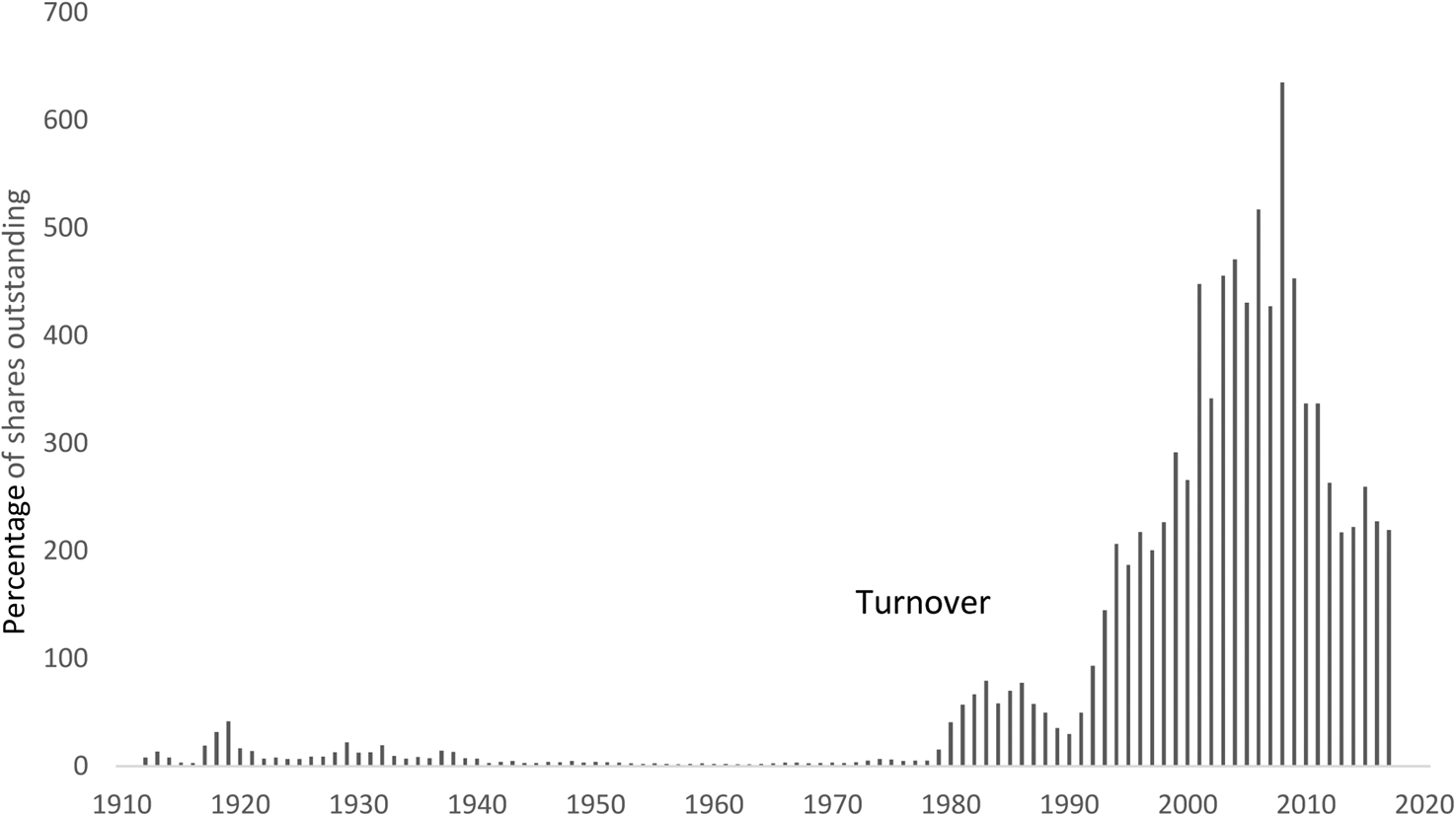
Figure 3. Stock market turnover 1912–2017

The figure plots stock market turnover as a percentage. For each day, we compute the value-weighted average of the number of shares traded divided by the number of shares outstanding. When a company has multiple classes of shares outstanding, we aggregate trading volume across classes and divide by the number of shares across all classes. When a stock has zero trading volume, we use the most recent market value as weight, and when a stock does not have any previous price information, we replace the missing market value with capital (par value times the number of shares). For each year, we compute the equal-weighted average turnover across days in the year.

Figure 4. Brokerage commission and transfer tax 1912–91

The figure plots brokerage commission and transfer tax as a percentage of the transaction price. Both the buyer and the seller must pay those charges. We do not have data on brokerage commission for 1992–2017. Data are taken from Waldenström Reference Waldenström2014.

Sweden has a bank-dominated financial system; Sweden's banking sector is roughly twice as large as the stock market, whereas the banking sector of the United States is about 25 percent of stock market capitalization (Figure 5). In the early days of stock market history, the relative size of the banking sector versus the stock market was even bigger because banks financed stock market investments. The official bank statistics divide the aggregate loan portfolio of banks into loans against real estate, stocks, bonds, personal guarantee and a residual. From 1912 to 1932, loans to finance stock purchases constituted about one-third of all bank lending and, as a result, banks owned approximately 40 percent of the stock market through loans against stocks.

Figure 5. Stock market capitalization, banking sector and the economy

The figure plots the ratio of stock market capitalization to GDP (dark grey column bars below) along with the aggregate balance sheet of commercial banks as a percentage of GDP (dashed line above). The balance sheet of commercial banks is taken from the Yearbook of Statistics Sweden.

Business loans were not reported as a separate item in the official bank statistics. To the extent that there were business loans, they were included in the residual. A glance at corporate balance sheets also suggests that banks did not lend directly to businesses. Figure 6 displays the time-series of new issue volume as a percentage of stock market cap. New issue volume was particularly high from 1912 to 1932, when bank loans against stocks represented a large portion of stock market capitalization. These three facts, (i) the extent of bank loan financing of stock purchases, (ii) the evolution of new issue volume and (iii) the non-reporting of business loans in the official bank statistics, suggest that banks financed businesses through the primary equity market.

Figure 6. New issue volume

The figure plots the annual new issue volume as a percentage of market capitalization. All new issues are rights offers of seasoned shares. There are no initial public offerings (IPOs).

From 1912 to 2017, firm size increased nearly 30 times (Table 2). Average firm size grew at approximately the same rate as GDP, which also increased nearly 30 times over the same time period. GDP growth can be divided into GDP per capita growth, which we think of as improvement in technology, and population growth. The former increased about 15 times, while the latter doubled. The increase in firm size and GDP per capita growth suggest that economies of scale through improved technology are the primary source of wealth creation.

Table 2. Firm size and the economy

The table reports real growth rates in percentages. Firm size, GDP and GDP per capita have been deflated by the consumer price index. The multiple denotes the ratio of the end value in 2017 to the beginning value in 1912. We estimate the growth rate in the number of shareholders from the number of bidders in rights offers 1912–20 and the number of shareholders as reported in the annual reports of a subset of firms. Statistics Sweden provides GDP and population statistics.

Over the same time period, the shareholder base expanded much faster (66.3 times) than the population (1.82 times). The growth rate in the number of shareholders (4.2 percent) also exceeded the growth rate in firm size (3.2 percent) and GDP per capita (2.6 percent). These numbers imply that initial shareholders exit the stock market and new shareholders enter the stock market when average income increases. Stock ownership is not once and for all a privilege of a wealthy class of households, but it disperses across the economy as average income increases. In other words, stock ownership is a normal good: old shareholders divest to increase consumption and new shareholders invest to increase savings.

II

We derive annual geometric average growth rates from a monthly stock price index. The stock market index reflects total stock returns, it includes dividends that are reinvested in the index, and it is value weighted. We include a return observation in the index only when we observe a transaction price from the last day of each of two adjacent months. Appendix A (available online) contains all measurement details, and Appendix B (online) analyzes the effects of stock selection, replacing missing prices with limit orders or past prices, and omitted split factors.

Table 3 summarizes stock market performance over the entire period 1912–2017, the historical portion of the data for 1912–78, and the modern portion for 1979–2017. The time-series of stock returns of companies listed on the Stockholm Stock Exchange exhibit all familiar characteristics. Stock and bond returns are positive, and stocks perform better than bonds. The equity premium is large and statistically different from zero with a t-statistic of 4.1. Compared to other countries with long time-series of stock returns, the average real rate of return of Swedish stocks in the amount of 7.77 percent is among the highest. The geometric average real rate of return on stocks over the time period 1900–2015 for the world is 5.0 percent, Europe 4.2 percent, United States 6.4 percent and United Kingdom 5.4 percent (Dimson et al. Reference Dimson, Marsh and Staunton2016). The average real interest rate in Sweden in the amount of 1.25 percent is comparable to the United States 0.8 percent and United Kingdom 1.0 percent (Dimson et al. Reference Dimson, Marsh and Staunton2016). The Sharpe ratio of 0.400 is high, and the equity premium is accordingly large.

Table 3. Stock market performance

The table reports performance statistics for the stock market, the bond market and the economy. The total return is the geometric average annual growth rate derived from a monthly stock price index. We deflate with the consumer price index. The equity premium is the difference between the total return and the bond market return. We represent the bond market interest rate by the discount rate of the Central Bank. From 1983, we use the Treasury bill rate taken from the Federal Reserve Bank of St Louis.

We estimate the coefficient of relative risk aversion by means of the following equation (Mehra Reference Mehra2003):

(1)$${\rm Equity\;premium} = \gamma \times {\rm Var( GDP) }, \;$$

where γ is the coefficient of relative risk aversion and Var(GDP) = 0.149 percent is the variance of real GDP growth. Our estimate of the coefficient of relative risk aversion exceeds reasonable values. Numerical calculations suggest that an investor with such a high value of relative risk aversion will invest next to nothing in the stock market regardless of wealth and time horizon (Jagannathan and Kocherlakota Reference Jagannathan and Kocherlakota1996).

Average stock returns are much higher in the modern portion of the data set for the period 1979–2017. This is interesting because the economy grows at a high rate throughout time. Figure 7 plots the real stock market index. It emphasizes (i) the persistent and strong stock price performance since 1934, (ii) the structural break in average stock market returns around 1979 (the slope of the line changes) and (iii) the strongly negative but short-lived effects of the Deflation Crisis (1920–1), when the stock price index decreased by 70 percent, and the Great Depression (1932–3), when the stock price index dropped by 65 percent. Business cycle effects are temporary and small in relation to the long-term growth of stock returns. Other crisis events such as World War II (1939–45), the 1970s stagflation (1974–9), the breakdown of the Swedish banking sector (1990–2), the burst of the internet bubble (2000–1) and the Global Financial Crisis (2007–9) are barely visible in the plot.

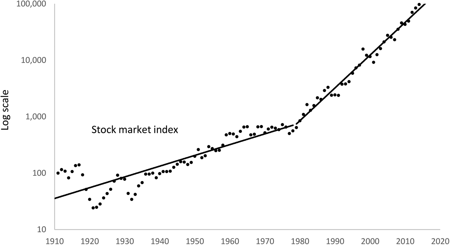
Figure 7. Real stock market index 1912–2017

The figure plots the level of the real stock market index (dots) along with trend lines for 1912–78 and 1979–2017. We deflate with the consumer price index.

The structural break in the time-series of stock returns is also visible in Figure 5 above. The ratio of stock market capitalization to GDP decreased from 1912 to 1978, when average stock returns were less than GDP growth, and the ratio increased from 1979 to 2017, when stock returns exceeded GDP growth. The banking sector also grew at a lower rate than the economy before 1979. Possible explanations for the structural break are the topic of Section iii below.

Table 4 decomposes stock returns into dividends and capital gains. The average dividend yield is 4.00 percent. Consistent with basic theory, the average capital gains yield 7.80 percent is close to the dividend growth rate 7.47 percent that we compute from the time-series of aggregate dividends. The dividend yield decreases over time from 4.30 percent measured over the period 1912–78 down to 3.52 percent over the period 1979–2017, and the capital gains yield increases from 2.13 percent to 15.57 percent over the two subperiods. Most listed companies pay dividends, and from 1949 to 1963, every listed company paid dividends (Figure 8). The U-shaped time path of dividend omissions resembles that of the United States (Fama and French Reference Fama and French2001). The higher frequencies of dividend omissions in the early years are the result of the Deflation Crisis and the Great Depression, and the increase in the percentage of non-payers in recent years reflects the change in the composition of companies away from manufacturing and forestry to biotechnology and information technology.

Figure 8. Companies that do not pay dividends 1912–2017

The figure plots the percentage of listed companies that do not pay dividends in a given year.

Table 4. Dividends and capital gains 1912–2017

The table breaks up the total stock return into dividend yield and capital gains yield. It also reports the geometric average dividend growth rate derived from the time-series of aggregate dividends. GDP is taken from Statistics Sweden. The inflation rate is derived from the consumer price index.

Figure 9 displays the evolution of the top statutory tax rate, the marginal tax rate of a household investor with annual income equal to ten times GDP per capita (GDP10), and the marginal tax rate of this investor multiplied by the household ownership fraction (weighted GDP10). As in the United States, there were two significant tax reforms, one that raised marginal tax rates in preparation for World War II and another that reduced marginal tax rates in 1991. Before World War II, the top statutory tax rate applied to very high income levels (income multiples between 53 and 756 times GDP per capita). After World War II, the top statutory tax rate became the relevant marginal tax rate for many households as tax tables were non-indexed and the forces of inflation and real income growth pushed households into higher income brackets (a process known as bracket creep). The GDP10 household hit the top income bracket in the 1960s. Possibly as a response to higher income tax, the household sector decreased its ownership share and the gap widened between the marginal tax rate of the GDP10 household and the weighted average marginal tax rate of the household sector (weighted GDP10).

Figure 9. Marginal tax rates

The figure displays the evolution of the top statutory rate on dividends (solid line above), the marginal tax rate associated with an annual income of ten times GDP per capita (GDP10; dashed line), and the same income multiplied by the aggregate stock ownership fraction of households (weighted GDP10; grey column bars). Dividends are exempt from personal income tax in 1994.

Personal income tax on dividends reduces annual stock market returns by approximately one percentage point (Table 5). The effect of income tax is fairly small despite high marginal tax rates on dividends from World War II to the tax reform of 1991. The explanation for the limited effect of high marginal tax rates on stock returns is that high-income households leave the stock market when marginal tax rates increase after World War II (Rydqvist et al. Reference Rydqvist, Spizman and Strebulaev2014).

Table 5. After-tax returns 1912–2017

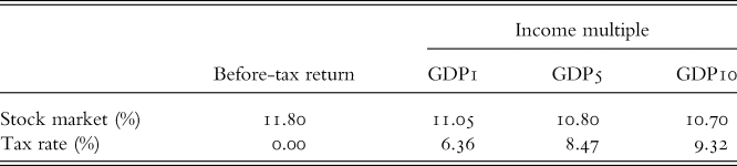
The table reports geometric average stock returns after tax along with the effective tax rates that we impute from the difference between before-tax and after-tax returns. GDP1, GDP5 and GDP10 denote the marginal tax rate associated with an income multiple of one, five and ten times GDP per capita, respectively.

Few previous papers analyze after-tax returns. Fisher and Lorie (Reference Fisher and Lorie1977) compute after-tax returns with a methodology similar to ours. From 1925 to 1976, US annual stock returns averaged 9 percent before tax; they were 8.3 percent after subtracting personal income tax on dividends at the income level GDP3 (low tax example), and 7.2 percent at income level GDP17 (high tax example). The authors do not take into account the fact that stock ownership migrated from the household sector to pension funds and insurance companies (Rydqvist et al. Reference Rydqvist, Spizman and Strebulaev2014). Siegel and Montgomery (Reference Siegel and Montgomery1995) extended their time-series from 1925 to 1993, when income tax reduced stock returns by approximately two percentage points. Finally, Siegel (Reference Siegel1994) reports after-tax returns based on the assumptions that shareholders pay the top statutory rate on both dividends and capital gains, and that shareholders do not exercise their options to defer capital gains and realize losses. Based on those assumptions, average stock returns decrease by approximately four percentage points in the US time-series.

III

Stock market performance was much stronger after 1978. We analyze three potential forces: (i) the growth of the public sector crowded out the private sector, which depressed the stock market; (ii) the entrance of foreign investors raised stock prices to international levels; and (iii) changing industry composition had no effect on stock prices.

Tax revenues as a percentage of GDP increased monotonically from 8.4 percent in 1912 to level out around 45 percent from 1979 to 2017 (Figure 10). These numbers suggest that the public sector grew at the expense of the private sector. Simply put, the taxation of income depressed the stock market from 1912 to 1978. Crowding out is a plausible argument in a small economy that was confined by natural geographic borders in the past and by capital controls from the outset of World War II. While companies expanded globally after World War II to exploit economies of scale, domestic investors being subject to harsh income tax did not have the resources to bid up domestic stock prices. Once currency controls were removed, international investors entered to bid up stock prices to intrinsic values.

Figure 10. Tax revenues to GDP

The figure plots the ratio of tax revenues to GDP as a percentage. Data are taken from Ekonomifakta.

The break point in the time-series of stock returns coincides with the removal of capital controls across Europe and the globalization of financial markets in the 1980s. Foreign investors initially entered the Swedish stock market in the 1920s, when Ivar Kreuger's companies (Kreuger & Toll, Tändsticksbolaget, LM Ericsson, and SKF) placed large volumes of shares in foreign stock markets (Figure 11). We estimate the foreign ownership fraction for these years by dividing the new issue volume to these companies by stock market capitalization. From the beginning of World War II on 1 September 1939 until 1989, the Central Bank exerted currency control, and the foreign ownership fraction decreased. In order to purchase Swedish shares, a foreign investor was obliged to sell Swedish shares in the same amount. The transaction amount is referred to as switch currency. The same restriction applied to a Swedish investor who wanted to purchase foreign shares: he had to sell foreign shares to acquire the necessary switch currency to pay for the foreign shares that he wanted to own. Foreign investors were allowed to sell shares back to Sweden, and Swedish investors were free to sell shares to foreign investors. These restrictions imply that foreign holdings of Swedish stocks and Swedish holdings of foreign stocks were limited to the outstanding stock at the beginning of World War II, and then decreased over time as Swedish shares were sold back to Sweden and foreign shares flowed out from Sweden. The purpose of these restrictions was to limit the outflow of Swedish currency that would otherwise be the consequence of (i) firms paying cash dividends to foreign investors and (ii) foreign sales of shares back to Sweden over and above the sale back of the initial stock from 1940. After all capital controls had been removed by Sweden and other European countries, the foreign ownership fraction increased to about 40 percent.

Figure 11. Foreign ownership fraction

The figure plots the foreign ownership fraction of listed Swedish stocks as a percentage. Data for 1975–2017 are taken from Statistics Sweden, while the point estimates for 1924–32 are based on new issue volume of class B shares and participating debentures divided by stock market capitalization at the beginning of the year. Data for 1933–82 are mostly missing.

The effects of capital controls are visible in Swedish stock prices. In 1916, the Government passed legislation that restricted foreign ownership to 20 percent of the voting rights. The purpose was to prevent foreign residents from ownership of Swedish domestic property and mines. Companies complied with the regulation by issuing one class of shares that was restricted to domestic ownership and another class of shares that anyone could own (unrestricted shares). From 1936 to 1939, unrestricted shares commanded a noticeable premium over restricted shares (Figure 12). Then, the currency regulation largely eliminated the foreign ownership premium until 1980, when the Central Bank issued more switch currency to allow foreign investors to increase their holdings of Swedish shares. The foreign ownership premium increased to very high levels; in some cases, the unrestricted shares up to 100 percent above the restricted shares. The foreign premium decreased in 1989, when the Central Bank abandoned all capital controls, and the foreign premium disappeared altogether in 1993, when all shares became eligible for foreign ownership.

Figure 12. Premium for unrestricted shares

The figure plots the evolution of the price difference between shares that are eligible for foreign investors as a percentage of an otherwise equivalent share that is restricted to domestic ownership. The number of voting rights is the same. The foreign ownership restriction was introduced in 1916 and removed in 1993. The first price pair is observed in 1936.

Industry composition has changed over time from manufacturing and natural resources (forestry and iron) to biotechnology and information technology. In Table 6, we report average stock returns by industry and subperiod. Stock returns have increased uniformly in recent years across industries. These numbers imply that the performance increase in recent years is the result of changing market conditions rather than a change in industry composition.

Table 6. Stock market performance by industry

The table reports performance statistics by industry. The total return is the geometric average annual growth rate derived from a monthly stock price index, and the equity premium is the difference between the total return and the bond market return.

IV

The article estimates average stock returns in a newly constructed data set of daily transaction prices and volume data from the Stockholm Stock Exchange for the period 1912–78, which we have merged with the previously existing database from 1979. The performance of the Stockholm Stock Exchange over more than 100 years, especially over the last 40 years, has been one of the strongest in the world. The market has developed from being extremely thin with only a handful of stocks that trade regularly to a stock market with daily transaction volume across the board. We base all calculations on scant transaction prices. Based on the analysis in Appendix B (online), we conclude that replacing missing prices with limit orders and past prices makes little differences to performance measurement as long as the stock market index is value-weighted. We urge other researchers to put effort into calculating split factors, when information is difficult to come by, because not correcting for stock splits, stock dividends or rights offers makes a significant difference in the performance measurement also for a value-weighted, broad stock market index.