1. Introduction
The central question of this paper is which linguistic primitive, markedness (Jakobson Reference Jakobson1932) or frequency (Haspelmath Reference Haspelmath2006), provides a better explanation for the relationship between grammatical gender and conceptual gender for certain noun pairs in English such as actor/actress and prince/princess. Before exploring this, we wish to first clarify the terminology that we have adopted to formulate this question. We use the term grammatical gender to refer to a property of linguistic forms, defined in morphosyntactic terms. Though English does not have grammatical gender for common nouns in the traditional linguistic sense, we continue to use that term here because it underscores the fact that the phenomenon that we study here in English also occurs in languages with traditional grammatical gender, and follows the grammatical gender opposition in those languages. Following Ackerman Reference Ackerman2019 (building on McConnell-Ginet Reference McConnell-Ginet and Corbett2015 and much other work), we use the term conceptual gender to refer to a property of ‘meaning’, broadly understood as a classificatory property, which Ackerman (Reference Ackerman2019: 3) characterizes as ‘the gender that is expressed, inferred, and used by a perceiver to classify a referent’. (Though it will not be relevant for our study, we note for completeness that Ackerman Reference Ackerman2019 further proposes the term biosocial gender to refer to the gender of a person, which may differ from the conceptual gender a speaker uses in classifying someone.) The asymmetrical relationship between grammatical gender and conceptual gender for the noun pairs that we explore here, first famously observed by Jakobson (Reference Jakobson1932), appears to be characterizable using two values for grammatical gender, [feminine] and [masculine], and two values for conceptual gender, [female] and [male]. Though we continue to adopt this apparent binarity in the construction and interpretation of our experiments, in part since the grammatical contrasts of interest are currently binary, we do not intend this apparent binarity to imply anything about the range of values that conceptual gender (or biosocial gender) can take, or the range of meanings that the linguistic system could potentially encode.
Our starting point is the observation that there are certain pairs of nouns that have distinct grammatical forms that appear to map in potentially complex ways to conceptual gender (Jakobson Reference Jakobson1932; see Corbett Reference Corbett1991). These pairs can be formed in at least three ways: (i) by a regular morphological alternation involving the suffix -ess, as in actor/actress; (ii) by an irregular alternation, typically involving -ess plus some additional phonological changes, as in headmaster/headmistress, and (iii) by the pairing of two morphophonologically distinct forms (suppletion), as in landlord/landlady. Crucially, in English, gender noun pairs appear to fall into two classes with respect to the meanings that the grammatically masculine form can take: in symmetric nouns, as in prince/princess, the grammatically masculine form can only be used to refer to a referent with male conceptual gender; in asymmetric nouns, the grammatically masculine form can either be used to refer to a referent with male conceptual gender or be used to refer to the superordinate category including both conceptual genders (including to a referent with unknown conceptual gender). In both classes, the grammatically feminine form can only refer to a referent with female conceptual gender. The first class is called symmetric because both nouns in the pair behave identically – they each refer to one specific conceptual gender. The second class is called asymmetric because the two nouns in the pair behave differently – the grammatically masculine form has two meanings, while the grammatically feminine form only has one. Table 1 provides examples of each morphological type for each class.
Table 1 Examples of gender noun pairs in English

Evidence for the behavior of these noun pairs usually comes from dialogues as in (1)–(2) for symmetric pairs and (3)–(4) for asymmetric pairs.


These dialogues assume that speaker in (a) is not aware of the conceptual gender of the people in the photograph, but is aware of the conceptual genders conventionally associated with the proper names in the (b) responses. A similar diagnostic obtains with plural forms, as has long been noted (e.g. Greenberg Reference Greenberg1966: 30–31, citing earlier Arabic grammarians; but see Chapter 9 in Corbett Reference Corbett1991 for critical discussion and examples that pattern differently).
Jakobson (Reference Jakobson1932) was the first to suggest that the asymmetric behavior of noun pairs like actor/actress (for a number of languages including German and Russian) was a part of a general notion of markedness asymmetries, being developed for phonological contrasts within the Prague School. Under the Jakobsonian approach, the form actress is morphologically ‘marked’, in the simplest sense, relative to the unmarked form actor, since actress bears a mark (the suffix -ess) that actor does not. Jackobson’s important insight was the proposal that there is a semantic markedness that parallels the morphological markedness: rather than saying there are two equal values for the semantic category of (conceptual) gender – female and male – Jakobson argued that the form actress is semantically marked for female conceptual gender, but that actor is semantically unmarked for conceptual gender. In other words, where the grammatically feminine form (suffix -ess) signals female conceptual gender, the grammatically contrasting masculine form (with no suffix) does not signal the opposite category, but instead simply makes no assertion about (conceptual) gender. Jakobson generalized from such examples, proposing further that the presence versus absence of an affix is only one manifestation of a more abstract sense of markedness. Thus, relevant to the examples at hand, his proposal is that the grammatical feature pair feminine:masculine is always marked:unmarked in languages like English, German, Russian, French, etc., even where it is not as neatly morphologically encoded as in actress:actor.
In contexts where the grammatically masculine (morphologically unmarked) form appears to denote the specific semantics of male conceptual gender, Jakobson proposes that some sort of logical reasoning is in the background: by selecting the unmarked form in a context where the marked form was in principle available, the speaker implies that they did not intend the marked form, and therefore did not intend the semantics of the marked form. Thus, in context, the morphologically unmarked form may come to imply the negation of the marked semantics (not-female conceptual gender), and thus, in a binary system, the unmarked form implies male conceptual gender, but this implication is not part of the meaning of the unmarked form. Finally, it is interesting to note that under the Jakobsonian approach, symmetric pairs are the relatively unexpected class. The fact that the grammatically masculine form only denotes a conceptually male referent in examples like (1) must mean that it is semantically marked conceptually male despite being morphologically unmarked. This must be something that is learned about these specific lexical items.
Since Jakobson’s (Reference Jakobson1932) seminal proposals, markedness has been a prominent explanans for the behavior of gender noun pairs across languages (e.g. Bobaljik & Zocca Reference Bobaljik and Zocca2011, Merchant Reference Merchant2014, Sudo & Spathas Reference Sudo and Spathas2016, and Saab Reference Saab, van Cranenbroeck and Temmerman2019, among others). However, there is at least one competing theory that attempts to explain these gender asymmetries without recourse to markedness. Haspelmath (Reference Haspelmath2006) proposes that the semantic asymmetries observed with the nouns in the asymmetric class (e.g. actor/actress) may be caused by asymmetries in the frequency of the two forms of the noun. (He embeds the discussion of gender noun pairs in a broader proposal to eliminate the concept of semantic markedness from the theory altogether.) Under Haspelmath’s theory, the asymmetry observed for actor/actress-class words occurs because the unmarked form (actor) is much more frequent than the marked form (actress), leading, in a way that is not completely specified, to a wider semantic meaning for the unmarked form. Similarly, the symmetry (or lack of asymmetry) for prince/princess-class words is due to the unmarked (prince) and marked (princess) forms having relatively equal frequencies. While Haspelmath’s short discussion is light on specifics, the relative frequency theory makes the strong prediction that as the relative frequency of the unmarked form over the marked form increases, so too should the asymmetry that we observe under the form:meaning diagnostics, like those in (3) and (4) above.
At a fundamental level, the markedness approach and the relative frequency approach make different empirical predictions, and it is these we set out to test. For the markedness approach, the lexical semantic representation of any given grammatically masculine noun, which is typically morphologically unmarked (except for widow/widower), has one of two options: either it bears the specification male conceptual gender or it is unspecified for conceptual gender.Footnote 2 Its behavior in frames such as the ones discussed above should either pattern with prince or with actor. There are two possible representations, so judgments should be categorical (in the ideal, i.e. up to speaker uncertainty, variation, and other sources of noise). Bobaljik & Zocca (Reference Bobaljik and Zocca2011) argue moreover that there is an internal unity to various semantic fields: profession nouns and animal names behave like the asymmetric actor/actress, and nobility titles and kinship nouns pattern like the symmetric prince/princess. By contrast, under the frequency approach, we expect to observe a far more gradient landscape, in which the judgments of semantic (un)markedness should correlate strongly with the relative frequency of the unmarked:marked (or grammatically masculine:grammatically feminine) members of the pair in some suitably representative corpus.
We test these predictions in two experiments designed to quantify the gender asymmetries. In the first experiment, we test a curated set of 16 noun pairs in English: eight putatively asymmetric (actor/actress-class) and eight putatively symmetric (prince/princess-class). In the second experiment, we test a set of 58 noun pairs that nearly exhausts the full set of such pairs in English. We then compare those quantified asymmetries to the relative frequency of the noun pairs as determined using the publicly available Corpus of Contemporary American English (COCA; Davies Reference Davies2008, March 2020 update).
The first step for these tests is to develop a quantifiable measure of gender asymmetry. To that end, we will adopt Bobaljik & Zocca’s (Reference Bobaljik and Zocca2011) ellipsis test for gender asymmetries. The underlying idea of the ellipsis test is that the identity requirement on ellipsis can be leveraged to uncover these asymmetries, and crucially, convert those asymmetries into unacceptability. Asymmetric nouns such as actor/actress display an asymmetry under ellipsis, as in (5):
The unmarked form (actor) can be the overt antecedent for an elided predicate that agrees with a conceptually female-biased name (5a), but the marked form (actress) cannot be the antecedent for an elided predicate that agrees with a conceptually male-biased name (5b). For symmetric nouns such as prince/princess, both combinations are unacceptable under ellipsis:
In this way, the Bobaljik & Zocca ellipsis test can be used to convert the gender asymmetry into an easily quantifiable acceptability effect that distinguishes two classes of nouns in English, while avoiding the methodological complexities that Jakobson’s original question/answer dialogues might raise (such as ensuring that participants read both sentences on each trial, and interpret them as coming from two distinct speakers).
We have three goals. The first is descriptive: to develop (and deploy) a formal experimental design for the Bobaljik & Zocca (Reference Bobaljik and Zocca2011) ellipsis test that we can then use to empirically determine the classes of noun pairs in English using the presence/absence of an asymmetry effect. The second is methodological: to evaluate Bobaljik & Zocca’s (Reference Bobaljik and Zocca2011) suggestion that ellipsis permits gender mismatches that are not otherwise tolerated. The third is theoretical: to use the quantified gender asymmetries from the two experiments to test the gradient predictions of the Haspelmath (Reference Haspelmath2006) relative frequency theory. With these goals in mind, the rest of this paper is organized as follows. In Section 2, we review the Bobaljik & Zocca analysis of the ellipsis test, and develop a factorial design that isolates the effect of each of the components of the Bobaljik & Zocca analysis. This will allow us to quantify each component, and crucially, isolate the gender asymmetry effect so that we can compare it to the relative frequency for each noun pair. In Section 3, we report the details of the first acceptability judgment experiment, which tests a curated set of 16 noun pairs that were chosen for their potential theoretical relevance. We test a very large number of participants per condition, and use a fully factorial design testing both ellipsis and non-ellipsis versions of the test sentences so that we can evaluate the viability of classifying noun pairs in English using the ellipsis test. In Section 4, we report the results of the second acceptability judgment experiment, which tests a set of 58 noun pairs that nearly exhausts the set of such pairs in English. Because of the large number of noun pairs, Experiment 2 tests a more typical number of participants per condition, and focuses exclusively on the ellipsis test conditions. The experimental materials and data sets for both experiments are available on the first author’s website. In Section 5, we compare the isolated gender asymmetry effect of each noun pair in both experiments with the relative frequency of each noun pair as calculated using COCA. Anticipating the results slightly, we find that (i) there are three noun pairs out of the curated set of 16 in Experiment 1 that behave differently than expected (though we offer some thoughts about why this may be); (ii) ellipsis is not required for mismatches to be tolerated (contra Bobaljik & Zocca Reference Bobaljik and Zocca2011); and (iii) the relationship predicted by the Haspelmath (Reference Haspelmath2006) relative frequency theory does not hold for the full set of noun pairs. Instead, we find that both classes of nouns are intermixed along the range of relative frequencies.Footnote 3 This suggests that the relative frequency theory is not an adequate empirical competitor with the markedness theory for explaining gender asymmetry effects. That said, we do find that some subsets of noun pairs could give the appearance of a relative frequency relationship, which may explain why the relative frequency theory appears plausible. Section 6 concludes with a summary of the findings, and a discussion of future directions for formal experimental investigations of gender asymmetry effects.
2. The ellipsis test for gender asymmetries
There are three components to the Bobaljik & Zocca (Reference Bobaljik and Zocca2011) analysis of the ellipsis test: (i) an identity requirement that holds between the antecedent and the elided material (see Merchant Reference Merchant, van Cranenbroeck and Temmerman2019 for a recent overview), (ii) a theory that acknowledges (at least) a three-way contrast in possible values for conceptual gender, even in a grammatically two-gender system, including ‘unspecified’ alongside ‘female’ and ‘male’, and (iii) some version of a principle like Maximize Presupposition (Heim Reference Heim, von Stechow and Wunderlich1991) or The Principle of Gender Competition (Sudo & Spathas Reference Sudo and Spathas2016). While these two principles differ in details, both give rise to a competition effect such that a more specified form blocks the use of a less specified form. Thus, in order to remain neutral about specifics we will simply refer to a ‘competition principle’. To make the discussion concrete, we will work through the five critical sentences previously presented in Section 1 before developing a formalization of the ellipsis test for our experiments.
We begin with an example without ellipsis, as in (7).
In (7a), the unspecified form of the noun actor is used, but the intended referent of the noun has female conceptual gender (indicated via the conceptual gender biased name Mary). Such an utterance is predicted to be judged infelicitous due to the competition effect generated via the existence of the more specified grammatically feminine form (7b).
Now, for ellipsis constructions containing the unmarked, and by-hypothesis unspecified, form of an asymmetric noun such as actor in (8a), there are two possible resolutions, as in (8b) and (8c) (material in angled brackets is interpreted but unpronounced).

In (8b), the unmarked form actor in the elided material satisfies the identity requirement. Furthermore, under the assumption that actor is unspecified for conceptual gender, there is no infelicity between Mary and actor. But the question arises – why is the use of actor in the ellipsis site in (8b) not blocked via competition with the more specific feminine form like we saw in (7a)? The idea pursued in Bobaljik & Zocca (Reference Bobaljik and Zocca2011) and Sudo & Spathas (Reference Sudo and Spathas2016) is that ellipsis bleeds the competition of the two forms, so a competition effect does not emerge when ellipsis takes place, hence (8b) does not incur a violation while the unelided (7a) does. In (8c), the marked resolution (actress) violates the identity requirement, so (8b) is the only grammatically licensed resolution for (8a). The existence of the resolution in (8b) means the sentence in (8a) is judged acceptable.
The converse configuration in (9a) also has two possible resolutions, as in (9b) and (9c).

In (9b), the unmarked resolution (actor) violates the identity requirement. In (9c), the marked resolution (actress) leads to infelicity because actress is marked (and therefore specified) conceptually female, while John is conceptually male-biased. Unlike (8), the sentence in (9) has no felicitous resolution, and is therefore judged unacceptable.
For symmetric nouns such as prince/princess in (10) and (11), there is no resolution that is both felicitous and grammatical.


Under the assumption that both forms of symmetric nouns are marked for conceptual gender, one of the two resolutions will be infelicitous, and the other will violate the identity requirement. Again, the key difference is in the lexical semantic representation of the morphologically unmarked terms: prince is semantically specified as conceptually male, while actor is unspecified for conceptual gender.
To formalize the ellipsis test, we constructed a 2 × 2 × 2 factorial design. Table 2 provides examples using the asymmetric pair actor/actress. At a descriptive level, what we manipulated was the grammatical gender of the predicate noun in the first clause and the conceptual gender bias of the subject of the second clause (i.e. by using stereotypically biased proper names). We note that the critical factors are not the specific values of grammatical gender and conceptual gender bias as such, but rather (i) whether the predicate noun in question is the grammatically masculine form, which is morphologically unmarked in the regular pairs, or the grammatically feminine form, which is morphologically marked in the regular pairs, and (ii) whether the predicate noun and the subject noun match in grammatical gender and conceptual gender bias or not. Therefore, we name these factors markedness and mismatch to better reflect the underlying logic of the design. Although this terminological choice superficially appears to favor the markedness theory over the relative frequency theory, we would like to note that this is simply a choice that will ultimately prove more convenient given our results. We could just as easily adopt the terminology of the relative frequency theory for our factors. The crucial question is whether the theories in question can explain the effects that obtain by manipulating the grammatical gender of the predicate NPs and the conceptual gender bias of the subject NPs in this systematic way.
Table 2 A 2 × 2 × 2 factorial design for the ellipsis test of gender asymmetries using the asymmetric pair actor/actress as an example.
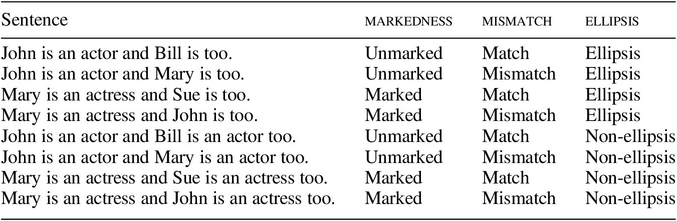
The primary manipulation in this design is the interaction between markedness and mismatch. When the predicate NP and subject NP match in grammatical gender and conceptual gender bias, we expect high acceptability, regardless of noun class. In this way, the match conditions form a baseline for highlighting the effect of mismatch. For symmetric nouns like prince/princess, we expect a mismatch between the predicate NP and subject NP in conceptual gender specification and conceptual gender bias to result in a decrease in acceptability for both the unmarked and marked form of the noun, as illustrated in the top left panel of Figure 1. This is the symmetry that characterizes symmetric nouns. For asymmetric nouns like actor/actress, we expect a decrease in acceptability for the marked mismatch condition (actress), but no decrease in acceptability for the unmarked mismatch condition (actor), as illustrated in the top right panel of Figure 1. This is the asymmetry that characterizes asymmetric nouns. In statistical terms, we expect a superadditive interaction between markedness and mismatch for asymmetric nouns like actor/actress, but no interaction for symmetric nouns like prince/princess.

Figure 1 Expected patterns for symmetric nouns (left panel) and asymmetric nouns (right panel), under ellipsis (top row) and non-ellipsis (bottom row).
We also included a secondary manipulation in the design to test whether ellipsis is necessary to reveal gender asymmetries by including a third factor, ellipsis, that manipulates the presence or absence of ellipsis. The Jakobsonian/Gricean analysis proposed by Bobaljik & Zocca (Reference Bobaljik and Zocca2011) predicts that symmetric and asymmetric nouns will show different patterns of acceptability in ellipsis constructions (top left panel versus top right panel in Figure 1), but the same pattern in non-ellipsis constructions (the bottom left and bottom right panels in Figure 1). However, Bobaljik & Zocca note that some speakers may not demonstrate the Jakobsonian/Gricean effect (i.e. some speakers may accept Mary is an actor). The non-ellipsis level of the factor ellipsis tests the Jakobsonian/Gricean analysis directly for the participants in our first experiment.
3. Experiment 1: A curated set of 16 noun pairs
In Experiment 1, we tested 16 noun pairs, eight that are by hypothesis asymmetric (actor/actress, waiter/waitress, god/goddess, widow/widower, heir/heiress, enchanter/enchantress, host/hostess, landlord/landlady), and eight that are by hypothesis symmetric (prince/princess, king/queen, count/countess, baron/baroness, uncle/aunt, brother/sister, husband/wife, brother-in-law/sister-in-law). There are three goals for Experiment 1. The first is to explore to what extent the class of each noun pair can be determined by the ellipsis diagnostic. We do this by looking for the presence or absence of a superadditive effect as described in Section 2. The second is to test whether the Jakobsonian/Gricean component of the analysis proposed by Bobaljik & Zocca is needed, that is, whether the difference between asymmetric and symmetric nouns emerges reliably only under ellipsis, or whether it might arise under non-ellipsis as well. The third is to quantify the size of the asymmetry effect (the superadditive effect) for each noun pair, and then test the relative frequency hypothesis. Though the nearly exhaustive set of 58 nouns in Experiment 2 will ultimately provide more information about the relative frequency hypothesis than this curated subset, the small number of noun pairs in Experiment 1 allows us to test a larger number of participants, and therefore establish extreme precision in the size of the asymmetry effect for these 16 noun pairs. With these goals in mind, we implemented the 2 × 2 × 2 factorial design in a seven-point Likert scale survey on Amazon Mechanical Turk. This section describes the details of the experiment and the results that we obtained.
3.1 The curated set of 16 noun pairs
We chose the curated set of 16 noun pairs using the following criteria. First, we used our native speaker intuitions to select noun pairs that are likely to be familiar to participants. Second, we chose nouns that can be used to describe humans, so we can leverage the conceptual gender bias of human names. Third, we used the suggestion in Bobaljik & Zocca (Reference Bobaljik and Zocca2011) that symmetric nouns form a semantic class comprised of nobility and kinship terms to select the noun pairs in the putative symmetric class. (These a priori class determinations will be quantitatively evaluated by the analysis below.) Fourth, we included both pairs respecting a regular morphological alternation (e.g. actor/actress) and pairs involving suppletion (e.g. landlord/landlady) in both groups because the literature on markedness makes no distinction between suppletion and overt morphology. Fifth, we also included the ‘markedness reversal’ pair widow/widower (Tiersma Reference Tiersma1982). It is a reversal in the sense that the morphologically marked form of most noun pairs refers to female conceptual gender, but for widow/widower, the morphologically marked form (widower) refers to male conceptual gender. If widow/widower shows a markedness asymmetry effect, we can ask whether it patterns according to morphological markedness (widow = actor) or according to markedness of conceptual gender (widower = actor).
3.2 Materials
We constructed eight conditions for each pair following the 2 × 2 × 2 design described in Section 2 and exemplified in Table 1. We created 8 lexically matched sets of items across the eight conditions (resulting in eight lexically matched tokens per condition) for each noun pair, for a total of 1024 target items. We constructed seven practice items that span the range of acceptability, including both agreement-centric constructions (both grammatical and ungrammatical) and other types of constructions. We also constructed 16 filler items that span the full range of acceptability, with eight that are agreement-focused, and eight that are of other types. The full set of materials is available on the first author’s website.
3.3 Design
We distributed the 1024 target items across experiments using a Latin Square design. Each survey contained one token of each of the eight conditions, while each condition in a survey used a different lexical item, with four lexical items from the asymmetric class and four from the symmetric class. Each survey included the seven practice items in the same order at the beginning of the survey (but not distinguished from the rest of the experiment), two filler items in the same order at the beginning of the main portion of the experiment, and then the eight target items and the remaining 14 filler items in a pseudorandomized order. Each survey was 31 items long (seven practice items, 16 filler items, eight target items), with a 2:1 ratio of filler items to targets (and a greater than 2:1 ratio of non-target items to targets). We constructed 128 distinct lists of items, and created four pseudorandom orders per list, for a total of 512 distinct surveys. The task was a seven-point scale task (1–7).
3.4 Participants
Three thousand and seventy-two participants were recruited using Amazon Mechanical Turk, resulting in six participants for each of the 512 surveys. Participants were paid $1.00 USD for their participation, which, given average completion times, resulted in an hourly rate of about $12.00 USD per hour. The distribution of surveys and participants yielded 192 judgments per condition per noun. The large sample size is, admittedly, more than necessary for this particular project; however, we plan to use these results as a baseline for future studies of gender asymmetries cross-linguistically. Other languages may not allow for such a high recruitment rate, so here we take advantage of the availability of so many participants in order to establish well-defined baseline distributions for these noun pairs.
3.5 Outlier identification and removal
Because the goal of Experiment 1 is to achieve an accurate and precise measure of the asymmetry effect for these 16 noun pairs, we employed a relatively strict outlier identification process. First, we removed participants who failed to affirmatively report being native speakers of US English. We included two language history questions for this purpose: (i) Did you live in the US from birth until age 13?, and (ii) Did your parents speak English to you at home? Participants were paid regardless of how they answered to encourage honest responses. We only retained participants who answered ‘yes’ to both questions for analysis; participants who responded ‘no’ or left the response blank in either question were removed from the analysis. This eliminated 198 participants (6.5%). Next, we used the 14 filler items that were interspersed with the target items (not the two items that were in a fixed position at the start of the main portion of the experiment) to identify uncooperative participants. We z-score transformed the responses for each participant to minimize the impact of common forms of scale bias. We then calculated means and standard deviations for each of the 14 fillers. We identified the participants whose responses were more than 2 standard deviations above or below the mean for each filler. We removed participants from the analysis if they were beyond this threshold for 2 or more of the 14 fillers (i.e. we only included participants who were beyond this threshold for at most one filler). This eliminated another 262 participants (8.5%). These two procedures left 2612 participants for the analysis (85% of those recruited). After this procedure, the target conditions in the experiment received between 132 and 190 judgments, with a mean of 163 judgments per condition.
3.6 Results
Figure 2 reports the mean ratings for each of the 16 noun pairs in Experiment 1 for all eight conditions: black lines for ellipsis conditions, gray lines for non-ellipsis conditions. We have organized the figure based on the a priori class of each noun pair (not based on the empirical results of our experiment). The top row contains putative asymmetric nouns, and the bottom row contains putative symmetric nouns. Recall that we expect asymmetric nouns to show a superadditive pattern as in the top right panel of Figure 1, and symmetric nouns to show two parallel downward sloping lines as in the left panel of Figure 1. We plot both ellipsis (black) and non-ellipsis (gray) here for completeness. In the discussions that follow, we will provide distinct ellipsis and non-ellipsis plots as appropriate.

Figure 2 Mean (z-score transformed) ratings for the 2 × 2 × 2 factorial design for the 16 noun pairs. The top row contains the putative asymmetric pairs; the bottom row contains the putative symmetric pairs. Both rows are roughly internally organized by the empirical results of the experiment, such that the interaction effect is decreasing for the asymmetric pairs (from most asymmetric to least), and increasing for the symmetric pairs (from most symmetric to least). Ellipsis conditions are in black; non-ellipsis conditions are in gray.
We constructed linear mixed-effects models for each noun pair with markedness, mismatch, and ellipsis as fixed factors, and item as a random factor (intercept only) using the lme4 package (Bates et al. Reference Bates, Maechler, Bolker and Walker2015) for the R language (R Core Team 2015). We could not include participant as a random effect distinct from the aggregate error term because, when looking at a single noun pair, each participant only rated one condition (i.e. within each noun pair the design is completely between participants). We could not include item slopes because each item (i.e. a full sentence) only appears in one condition. We used the lmerTest package (Kuznetsova, Brockhoff & Christensen Reference Kuznetsova2017) to perform hypothesis tests similar to omnibus ANOVAs for each noun pair using the Satterthwaite approximation of degrees of freedom. Because the omnibus tests are not part of any of the hypotheses that we are testing, we have placed the details of the omnibus tests in the appendix. Here in the main text we focus on the two specific (planned) 2 × 2 tests crossing markedness and mismatch within each level of ellipsis as required by the goals of the experiment.
3.7 Classifying the 16 noun pairs using the ellipsis diagnostic
The first goal of the experiment is to classify the noun pairs as either asymmetric or symmetric according to the pattern of acceptability that they display in the four ellipsis conditions (black lines). We plot the ellipsis conditions alone in Figure 3.

Figure 3 Mean (z-score transformed) ratings for the 2 × 2 factorial design for the 16 noun pairs for ellipsis conditions only (black lines from Figure 2). The top row contains the putative asymmetric nouns; the bottom row contains the putative symmetric nouns. Both rows are roughly internally organized by the empirical results of the experiment, such that the interaction effect is decreasing for the asymmetric pairs (from most asymmetric to least), and increasing for the symmetric pairs (from most symmetric to least). Each facet reports the p-value of the interaction term (the asymmetry effect) in the 2 × 2 linear mixed effects models rounded to three significant digits.
From visual inspection, we see that seven of the eight noun pairs in the top row appear to show the asymmetric pattern of judgments: actor/actress, waiter/waitress, heir/heiress, enchanter/enchantress, host/hostess, and landlord/landlady, and god/goddess. The pair widow/widower appears to show a small superadditive effect in the opposite direction than predicted. As noted above, we included widow/widower because it is a well-known example of a ‘markedness reversal’ in that the unmarked form refers to female conceptual gender. These results seem to confirm that widow/widower patterns differently than the other two classes. We return to this point briefly in Section 6. We also see that two of the noun pairs in the bottom row, count/countess and baron/baroness, fail to show the symmetry pattern: count/countess shows a non-monotonic interaction that is similar in consequence to the asymmetry pattern; baron/baroness shows a small asymmetry pattern. This is a potentially surprising result given that these two nouns are nobility titles, and other nobility titles demonstrate the symmetry pattern. We speculate that this may be a reflection of less familiarity with count(ess) and baron(ess) as nobility titles (and accordingly some speaker uncertainty in the semantic representation) for US-based participants. We return to this point briefly in Section 6.
To quantify these visual impressions, we constructed linear mixed-effects models (using treatment coding) with markedness and mismatch as fixed factors and item as a random factor (intercepts-only), but only within the ellipsis conditions. We again used the lmerTest package to calculate p-values using the Satterthwaite approximation of degrees of freedom. We can then look for significant superadditive interactions as an index of the gender asymmetry pattern. The p-values for the interaction terms appear in each facet of Figure 3. (The full results of the linear mixed effects models appear in the appear in the appendix.) To highlight the size of the asymmetry effects (the interaction term) for each noun pair, in Figure 4 we plot the size of the asymmetry effect, with the noun pairs ordered by the size of the effect, and statistical significance indicated by shading.

Figure 4 The size of the asymmetry effect (the interaction term in the 2 × 2 design) for the ellipsis conditions in Experiment 1. The noun pairs are ordered by descending asymmetry effect size. The statistical significance of the interaction term (by linear mixed effects models) is indicated by shading. Error bars represent estimated 95% confidence intervals.
The statistical results confirm what we see through visual inspection in Figure 3 and Figure 4: actor/actress, waiter/waitress, heir/heiress, enchanter/enchantress, host/hostess, and landlord/landlady, and god/goddess all show significant superadditive interactions indicative of the asymmetry pattern. Count/Countess and baron/baroness also unexpectedly show significant superadditve interactions indicative of the asymmetry pattern. Brother/sister-in-law, uncle/aunt, prince/princess, husband, wife, and brother/sister show no significant interaction, indicative of the symmetry pattern. King/queen does show a significant superadditive interaction, but in the opposite direction than predicted for an asymmetry effect. There is a small increase in acceptability for Mary is a queen and John is too over John is a king and Mary is too. This may be because of the multiple meanings of the word queen. Widow/widower also shows a significant non-monotonic interaction, again in the opposite direction to the predicted asymmetry pattern. There is a small increase in acceptability for John is a widower and Mary is too over Mary is a widow and John is too. This pattern requires further investigation. One possibility is that this is a true asymmetry effect, but aligned with gender, such that widower (masculine) is behaving as the other masculine forms (actor) even though it is morphologically marked relative to widow. That would be potentially theoretically interesting. However, this seems unlikely given that both mismatch conditions were rated relatively low, unlike the asymmetric noun pairs (where one mismatch condition is rated relatively high), and more like the symmetric noun pairs.
3.8 Evaluating the role of ellipsis in revealing gender asymmetries
The second goal of the experiment is to test the Jakobsonian/Gricean analysis proposed by Bobaljik & Zocca (Reference Bobaljik and Zocca2011). Their analysis predicts that the gender asymmetry pattern should disappear in the non-ellipsis conditions. The Jakobsonian/Gricean analysis predicts that the unmarked mismatch conditions for both asymmetric and symmetric nouns will violate a principle of the grammar: for symmetric nouns, there will be a gender clash in the second clause (John is a prince and Mary is a prince too); for asymmetric nouns, there will be a competition principle violation in the second clause (John is an actor and Mary is an actor too). However, based on the results of this experiment, these predictions do not appear to hold. Figure 5 shows interaction plots that isolate the non-ellipsis conditions (gray lines, as in Figure 2 above).

Figure 5 Mean (z-score transformed) ratings for the 2 × 2 factorial design for the 16 noun pairs for non-ellipsis conditions only (gray lines from Figure 2). The top row contains the putative asymmetric nouns; the bottom row contains the putative symmetric nouns. Both rows are roughly internally organized by the empirical results of the experiment, such that the interaction effect is decreasing for the asymmetric pairs (from most asymmetric to least), and increasing for the symmetric pairs (from most symmetric to least). Each facet reports the p-value of the interaction term (the asymmetry effect) in the 2 × 2 linear mixed effects models.
Asymmetric nouns in non-ellipsis conditions still show the asymmetry pattern. The p-values in each facet of Figure 5 report the statistical significance of the markedness × mismatch interaction. (The full statistical results for the non-ellipsis conditions are in the appendix.)
The presence of the asymmetric pattern suggests that participants in our study accepted sentences like John is an actor and Mary is an actor too for asymmetric nouns (the top right point in each of the plots in Figure 5), while rejecting this construction for symmetric nouns (*William is a prince and Anne is a prince too). To investigate this result in more depth, we plot the distribution of judgments for both the ellipsis and non-ellipsis versions of these conditions in Figure 6 (these are the distributions for the two top-right points in Figure 2 above). What we are looking for is evidence of bimodality in the non-ellipsis judgments (gray lines) for the asymmetric nouns. Bimodality would suggest that there may be two populations of speakers: those that accept Mary is an actor and those that reject it. However, we do not see any compelling evidence of bimodality in the distributions for the asymmetric nouns.

Figure 6 The distributions of judgments for the unmarked mismatch conditions for both ellipsis (John is an actor and Mary is too; black) and non-ellipsis conditions (John is an actor and Mary is an actor too; gray).
This result suggests that the role of the competition principle in the ellipsis and non-ellipsis constructions tested in this study is less substantial than Bobaljik & Zocca assumed, and that the difference between asymmetric and symmetric nouns can be seen without ellipsis (perhaps somewhat ironically, since ellipsis served as the initial focus of our study). The asymmetry of primary interest is the difference between symmetrical nouns, which tolerate no mismatch: #Mary is a prince, and asymmetrical nouns, which (in principle) should allow an unmarked noun to be predicated of a conceptually female-biased subject: Mary is an actor. Bobaljik & Zocca argued that this difference could be seen most clearly in ellipsis, since they held that the mismatch in Mary is an actor is disfavored when ellipsis is not involved. A Jakobsonian/Gricean logic involving competition of forms was offered to explain the reduced acceptability of sentences like Mary is an actor in non-ellipsis contexts, since in those contexts (but not in ellipsis contexts) a matching alternative is available: Mary is an actress. Our results are consistent with this role for the competition principle in regulating a preference when two alternatives are available, but the effect that it describes is very small; there may be a subtle preference for the matched form in non-ellipsis contexts (especially for nouns like goddess, hostess, and waitress), but our results indicate that it is wrong to think of sentences like John is an actor and Mary is an actor too as involving any kind of grammatical violation.
As a brief aside, Figure 6 also serves to highlight the three pairs that showed unexpected results: count/countess, baron/baroness, and widow/widower. The less peaky, and possibly bimodal, distributions in Figure 6 suggest that participants were split in whether to treat these as gender asymmetric or not.
There was also one unpredicted result in our experiment: there is an increase in acceptability of marked mismatch conditions under ellipsis (Mary is an actress and John is too; bottom right points of each plot in Figure 2 above) compared to their non-ellipsis counterparts (Mary is an actress and John is an actress too) for the asymmetric nouns. These are relatively small effects. Statistically speaking, these effects should appear as a three-way interaction among all three factors in our omnibus tests. However, given that these effects are so small, that three-way interaction only reaches significance for two noun pairs: actor/actress and host/hostess (see Appendix). Neither the Bobaljik & Zocca markedness theory nor the Haspelmath relative frequency theory predicts this amelioration effect of ellipsis. To investigate this effect a little more deeply, we plot the distribution of judgments for these two conditions in Figure 7. What we see is some bimodality in both conditions, ellipsis and non-ellipsis alike, with more pronounced bimodality in the ellipsis conditions for many of the asymmetric nouns. This suggests that there may be two populations of speakers when it comes to this unexpected amelioration effect of ellipsis: those that accept Mary is an actress and John is too, and those that reject it. As this effect was not part of the design of the current experiment, we note it here, and set it aside for future research.

Figure 7 The distributions of judgments for the marked mismatch conditions for both ellipsis (Mary is an actress and John is too; black) and non-ellipsis (Mary is an actress and John is an actress too; gray).
4. Experiment 2: A nearly exhaustive set of 58 noun pairs in English
Though it is in principle possible to look for a relationship between relative frequency and asymmetry effects with the curated set of 16 noun pairs tested in Experiment 1, an anonymous JL referee for an earlier version of this manuscript correctly observed that the non-random selection of those noun pairs could have inadvertently biased the relationship. To eliminate that possibility, we designed Experiment 2 to test a set of noun pairs that nearly exhausts the set of gendered pairs in English. In this section, we describe the acceptability experiment and its results. We then use the results from both Experiment 1 and Experiment 2 to test the relative frequency hypothesis in Section 5 .
4.1 The nearly exhaustive set of 58 noun pairs in English
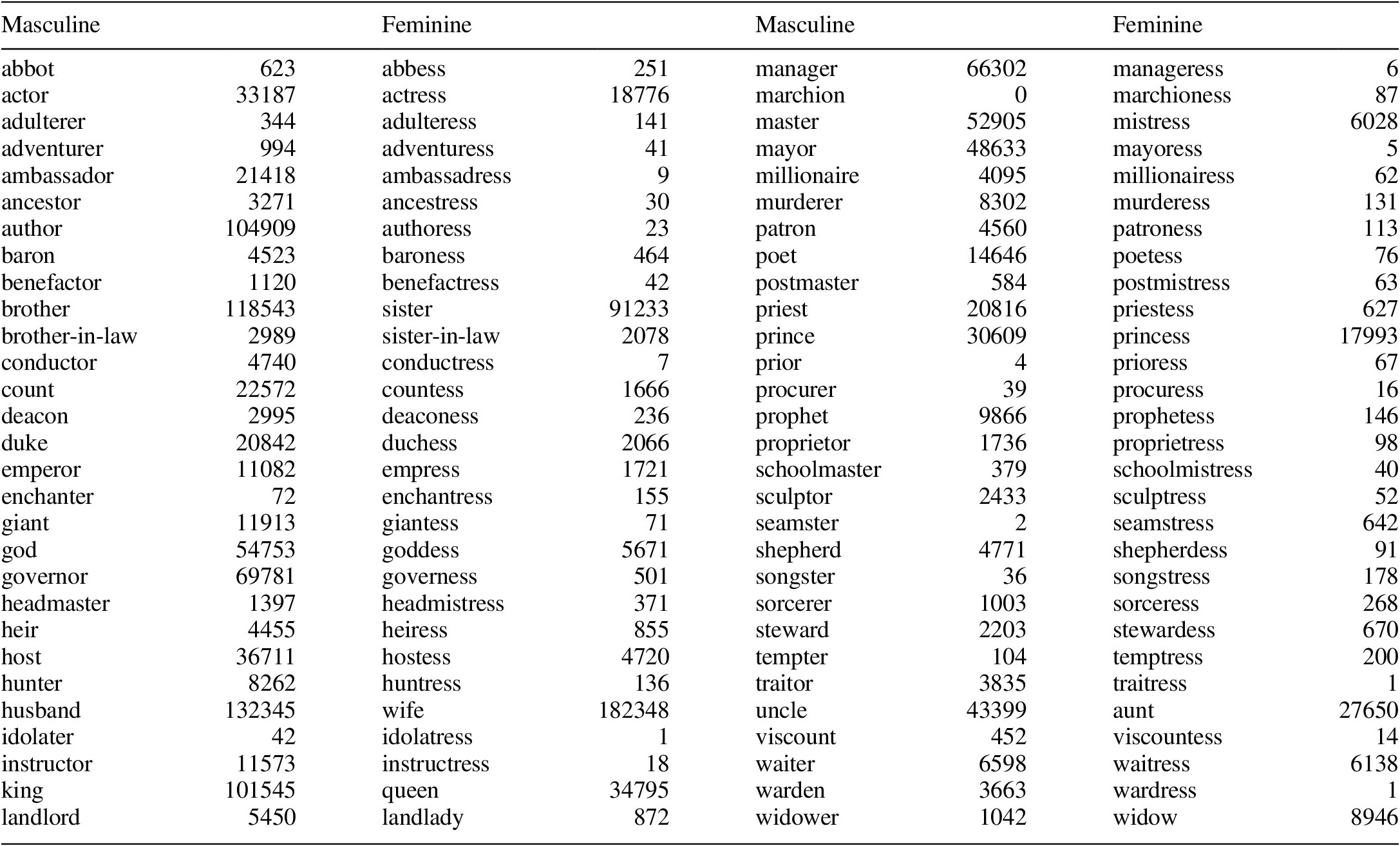
We first extracted all of the noun pairs involving -ess from the Reverse English Dictionary Based on Phonological and Morphological Principles (Muthmann Reference Muthmann1999), except for two that are slurs. We then added the six pairs from Experiment 1 that did not involve -ess, for a total of 58 noun pairs. Though there are likely additional noun pairs in English that we could have included, this set represents a substantial portion of the possible pairs in English, particularly for the regular -ess alternation. The full list of 58 nouns and their frequencies in COCA are listed in the appendix. The design of Experiment 2 was parallel to that of Experiment 1, with one change – we only tested the 2 × 2 ellipsis design. This change was for practical reasons. Testing 58 noun pairs necessarily requires a very large sample size. Since ellipsis and non-ellipsis designs yielded nearly identical results in Experiment 1, we decided to focus on only ellipsis (the original diagnostic from Bobaljik & Zocca Reference Bobaljik and Zocca2011) to double the rate of data collection.
4.2 Materials and design
We constructed eight conditions for each pair following the 2 × 2 design. We created eight lexically matched sets of items across the four conditions (resulting in eight lexically matched tokens per condition) for each of the 58 noun pairs for a total of 1856 target items. We selected 8 conceptually male-biased and eight conceptually female-biased names by consulting the list of most popular baby names for the 1980s, 1990s, and 2000s on the Social Security Administration website, and using our own intuitions to select names that were (i) uniquely biased with respect to conceptual gender, and (ii) as highly ranked as possible across all three decades (as these are the most likely decades of birth for participants on AMT). The mean rank of the conceptually male-biased names across the three decades is six; the mean rank of the conceptually female-biased names is 12. We used the same practice and filler items as Experiment 1. The full set of materials is available on the first author’s website. We distributed the 1856 target items across experiments using a Latin Square design. Each survey contained two tokens of each of the four conditions, with each token testing a different noun. The survey construction was otherwise identical to Experiment 1: 31 items long, seven practice items, eight target items, and 16 fillers. The task was a seven-point scale task (1–7).
4.3 Participants, outlier identification, and removal
Nine hundred and twenty-eight participants were recruited using Amazon Mechanical Turk. Participants were paid $1.00 USD for their participation, which, given average completion times, resulted in an hourly rate of $12.00 USD per hour. The distribution of surveys and participants yielded 32 judgments per condition per noun. We used the same outlier removal process as Experiment 1. One participant was removed for submitting two surveys. 36 participants were removed for failing to answer ‘yes’ to both language history questions. 168 participants were removed for rating 2 or more filler items more than 2 standard deviations above or below the mean rating. This left 712 participants for the analysis (77% of those recruited). After the outlier removal process, the target conditions in the experiment received between 20 and 30 judgments, with a mean of 24.5 judgments per condition.
4.4 Results and discussion
As in Experiment 1, we z-score transformed each participant’s judgments to eliminate common types of scale bias, then constructed linear mixed effects models using markedness and mismatch as fixed factors and item as a random factor (intercepts-only), and used the lmerTest package to calculate p-values using the Satterthwaite approximation of degrees of freedom. Figure 8 reports the size of the asymmetry effect for each of the 58 noun pairs, with the noun pairs ordered by the size of the effect, and statistical significance indicated by shading. The full statistical results are reported in the appendix. Though the primary purpose of Experiment 2 is to provide asymmetry effect sizes to use in our exploration of the prediction of the relative frequency hypothesis (Section 5), we provide the judgment results here for completeness.

Figure 8 The size of the asymmetry effect (the interaction term in the 2 × 2 design) for Experiment 2. The noun pairs are ordered by descending asymmetry effect size. The statistical significance of the interaction term (by linear mixed effects models) is indicated by shading. Error bars represent estimated 95% confidence intervals.
5. The relative frequency hypothesis
The Haspelmath (Reference Haspelmath2006) relative frequency hypothesis proposes that the asymmetric acceptability patterns for asymmetric nouns can be explained by the relative frequency of the two forms in any given pair. Haspelmath (Reference Haspelmath2006: 53) says:
to really explain what is going on, we need to refer to a variety of factors, among them clearly frequency of use: in the pair dog/bitch, bitch has a much lower proportional frequency than queen has in the pair king/queen, so it is not surprising that it behaves more like a hyponym of dog.
Though Haspelmath leaves the causal mechanism unstated under the phrase ‘it is not surprising that’, the descriptive idea seems to be that pairs with large differences in relative frequency are more likely to display the asymmetry pattern; and pairs with a smaller difference in relative frequency are more likely to display the symmetry pattern. We can test this prediction by looking for a correlation between relative frequency of the two forms and the size of the superadditive interaction in the two acceptability judgment experiments.
5.1 The mathematical details
We retrieved the frequency of the noun forms in our study from the Corpus of Contemporary American English (COCA), which consists of over 1 billion words (20 million per year from 1990 to 2019) collected from eight genres (Davies Reference Davies2008; accessed after the March 2020 update). The raw frequency counts for each noun in the 58 pairs are reported in the appendix. We (decadic) log-transformed the relative frequencies because this normalizes the logarithmic distribution of word frequencies in natural language. This also has the added benefit of making the numbers easy to interpret. The sign indicates the direction of the relative frequency of the marked form (e.g. actress): a negative sign indicates that the marked form is less frequent than the unmarked form (e.g. actress < actor); zero indicates that the two frequencies are equal (e.g. actress = actor); and a positive sign indicates that the marked form is more frequent than the unmarked form (e.g. actress > actor). The magnitude of the log relative frequency indicates the order of magnitude of the relative difference: −1 means that the marked form was 1/10 as frequent, −2 means that the marked form was 1/100 as frequent, −3 means that the marked form was 1/1000 as frequent, etc. We calculated the relative frequency in this direction (marked-to-unmarked) because Haspelmath (Reference Haspelmath2006: 53) phrases the relative frequency hypothesis in terms of the ‘low proportional frequency’ of the marked item in the pair. It would be informationally equivalent to calculate the relative frequency in the other direction (unmarked-to-marked), resulting in a sign change. Nonetheless, we choose to keep it in Haspelmath’s (Reference Haspelmath2006) terms for maximum compatibility with his formulation of the relative frequency hypothesis.
The relative frequency hypothesis states that marked forms that are relatively less frequent than their unmarked partner should lead to the gender asymmetry pattern. The mathematical prediction is thus that negative log relative frequencies should show larger superadditive judgment effects, and positive log relative frequencies should show smaller (or no) superadditive judgment effects. In other words, we are looking for a negative correlation between log relative frequency and the superadditive judgment effects – that is, a downward sloping line if both quantities are plotted from smallest to largest. We also expect the relationship between relative frequency and asymmetry effect size to be relatively strong. This is because the relative frequency hypothesis proposes a causal relationship between frequency and acceptability. Therefore, we provide two measures of the strength of the relationship. The first is a descriptive measure, R2, which measures the proportion of the variance between frequency and acceptability that is explained by the line of best fit. The second is an inferential measure, the Bayes factor, which measures the relative likelihood of the data under two hypotheses – the null hypothesis (H0) that there is no relationship and the experimental hypothesis (H1) that there is a relationship (see Morey, Romeijn & Rouder Reference Morey, Romeijn and Rouder2016 for a review). As a proportion, Bayes factors can be calculated in either direction. A BF01 measures how much more likely the data is under the null hypothesis. A BF10 measures how much more likely the data is under the experimental hypothesis. Because of the nature of our results, we either report BF01 alone or report both BF01 and BF10 together arranged symmetrically around 1. We used the Bayes Factor package in R to perform the calculations (Morey & Rouder Reference Morey and Rouder2018).
5.2 The correlations for Experiment 1 and Experiment 2
Figure 9 reports the correlation for both the ellipsis and non-ellipsis results from Experiment 1 for the curated set of 16 noun pairs. Though this is a curated subset, and therefore could suffer from bias, we include it here for completeness. Figure 10 reports the correlation for 57 of the 58 noun pairs from Experiment 2. We excluded marchion/marchioness because the frequency of marchion in COCA is 0. We plot three sets: the full set of 57 noun pairs, the subset of 39 pairs that stand in a regular morphological relationship (add -ess), and the subset of 18 pairs that involve either an irregular alternation (such as master/mistress) or suppletion (such as king/queen). This distinction is not made by the relative frequency hypothesis; we include these subsets for readers who may wonder if the regularity of the morphological relationship affects the results (it does not). In both figures, we report two correlations. The first is a correlation of the full set of points as expected. We report that correlation with a black line of best fit and statistics in a black font. In the second correlation, reported as a gray line of best fit and statistics in a gray font, we transform the negative asymmetry effects to 0 (a type of Winsorization). The logic behind this is that negative asymmetry effect sizes are not directly predicted by the relative frequency theory, so one may wonder if these negative effect sizes may be masking the predicted relationship. By transforming the effect sizes to 0, we minimize that masking. We add gray shading to indicate the points that were transformed.

Figure 9 Experiment 1. The correlation of log relative frequency between the marked and unmarked forms of each noun and the size of the asymmetry effect, defined as the size of the markedness × mismatch interaction, for the curated set of 16 noun pairs. Black lines and statistics are for the original data set; gray lines and statistics are for the Winsorized data set.

Figure 10 Experiment 2. The correlation of log relative frequency between the marked (e.g. actress) and unmarked (e.g. actor) forms of each noun and the size of the asymmetry effect, defined as the size of the markedness × mismatch interaction, for the nearly exhaustive set of noun pairs. Black lines and statistics are for the original data set; gray lines and statistics are for the Winsorized data set. The columns report distinct sets of the noun pairs.
The relative frequency hypothesis predicts a strong negative relationship between log relative frequency and the asymmetry effect: as the log relative frequency of the marked-to-unmarked form increases, the size of the asymmetry effect should decrease. But this is not what we find. Though the lines of best fit are negative in both Figures 9 and 10, for both the curated set and the exhaustive set of noun pairs, and for both the original data sets and the Winsorized data sets, the amount of variance explained by the line of best fit is exceedingly small, from less than 1% to 5% as indicated by the R2 values. Similarly, for all data sets, the Bayes factors favor the null hypothesis that there is no relationship between frequency and the asymmetry effect, with the data being between 3.55 and 4.95 times more likely under the null hypothesis. Qualitatively, we can see that the nouns with smaller asymmetry effects (y-axis) appear to be well-mixed among the range of relative frequency (x-axis). For example, prince/princess and actor/actress have nearly identical relative frequencies, yet are often used as contrasting examples to define gender asymmetry effects. In short, there is no clustering of the noun classes in different relative frequency ranges, suggesting neither a continuous nor a categorical separation of the noun classes based on relative frequency. This suggests that the relative frequency hypothesis cannot be a substantial component of the explanation of the gender asymmetry effects. Although this does not prove that the markedness-based theory is correct, it does suggest that relative frequency is not an empirically adequate competitor with semantic markedness for the explanation of gender asymmetry effects.
5.3 Resampling simulations
The nearly exhaustive data set from Experiment 2 allows us to look more deeply at the relationship between frequency and the asymmetry effect. Here we report two additional analyses using resampling simulations. The first resamples based on minimum frequency. Figure 11 reports the R2 and BF for the subsets of the noun pairs created by every possible minimum frequency between 1 and approximately 6000 in COCA. We plot the minimum frequency threshold along the x-axis, using raw counts spaced logarithmically for clarity. Because the subsets are based on increasing minimum frequency, the number of noun pairs in each subset decrease as the minimum frequency threshold increases. We plot one point for each unique subset that is created. The top row reports the R2; and the bottom row reports both BF01 and BF10 symmetrically around 1. The columns report the full set of 57 noun pairs, the subset of 39 pairs that stand in a regular morphological relationship, and the subset of 18 pairs that involve either an irregular alternation or suppletion.

Figure 11 R2 and BF01 for the subsets of the noun pairs in Experiment 2 created by every possible minimum frequency between 1 and approximately 6,000 in COCA. The top row reports the R2; and the bottom row reports both BF01 and BF10 symmetrically around 1. The columns report three sets of the noun pairs.
Turning first to the set of all nouns, we see that the overall pattern of no relationship between frequency and the asymmetry effect holds for most of the possible subsets defined using minimum frequency thresholds. We see this both in the low R2 values and the Bayes factors that favor the null hypothesis. There are only two small zones in the plot that could give the appearance of a relationship between relative frequency and the asymmetry effect – one is around a minimum frequency threshold of 100, and the other is around a threshold of 2000. Those thresholds lead to maxima in the R2 plot and to Bayes factors that favor the experimental hypothesis. This is potentially interesting in that it raises the possibility that the relative frequency approach may appear more or less reasonable based on the specific subset of the nouns that one is looking at.
Turning next to the subset of noun pairs that demonstrate a regular morphological relationship, we see small R2 values and Bayes factors that favor the null hypothesis uniformly from a minimum frequency threshold of 1 to a minimum frequency threshold of 2000. Around 2000 we see an increase in R2, but the Bayes factors are near 1, suggesting that the data in these subsets is roughly equally likely under both hypotheses. We interpret this to indicate that the relatively small number of noun pairs in the subsets at this minimum frequency threshold leads to insufficient sensitivity in these measures. A similar issue arises for the irregular and suppletive subset. As the number of noun pairs in the subset decreases (from a maximum of 18 at a minimum frequency threshold of 1), we see increases in R2 values that are accompanied by Bayes factors near 1, suggesting insufficient sensitivity to favor one hypothesis over the other.
For a second analysis, we set aside the idea that the subsets could only be formed through a frequency threshold, and instead sampled freely from each set of noun pairs. We performed analyses at two sample sizes – samples of size 20 for the set of all noun pairs and regular morphology noun pairs and samples of size 10 for the irregular and suppletive noun pairs. We chose these sample sizes because they are roughly half of the size of the regular (39) and irregular and suppletive (18) subsets, and would thus lead to reasonable variability across samples. We repeated the resampling procedure 10,000 times for each sample size. Figure 12 is a set of histograms for those resampling simulations, showing the percentage of samples that yielded each R2 and BF value.

Figure 12 Histograms for random sampling simulations at sample sizes of 20 and 30, based on the data set for the noun pairs in Experiment 2. The top panels report the R2; and the bottom panels report both BF01 and BF10 symmetrically around 1. The columns report three sets of the noun pairs.
The overwhelming pattern, for all three sets of noun pairs, is that the R2 values are relatively small, and the Bayes factors strongly favor the null hypothesis. This suggests that, even though it is possible to hit upon a few special subsets of noun pairs that will yield the appearance of a strong relationship between relative frequency and asymmetry effects, particularly if the subsets are constructed based on minimum frequency thresholds, this is not the true underlying pattern in the data. Instead, it appears as though there is no substantial relationship between relative frequency and the asymmetry effects (regardless of the morphological relationship within the pairs).
6. A note on indeterminate categories in a (binary) markedness approach
Our results broadly support the categorical (in fact, binary) markedness approach over the more gradient frequency approach. However, noun pairs like baron/baroness, count/countess, and widow/widower from the curated set in Experiment 1 do not quite fit neatly into the two patterns predicted by the markedness approach: they show superadditive interactions like asymmetric nouns, but the acceptability of the mismatched conditions are relatively low like symmetric nouns. The question we raise briefly in this section is whether a binary markedness system can account for noun pairs that do not fit neatly within either of the predicted patterns. We believe the answer is yes, but it requires a closer look at the role of semantic fields in the markedness system.
To a first approximation, Bobaljik & Zocca suggested that semantic fields correlate in different ways with semantic (under)specification for conceptual gender. This claim is substantially borne out by these results, modulo the three exceptions noted above. Crucially, semantic fields (such as profession names, kinship terms, and nobility titles) are not a part of the linguistic representations we assume, but are instead cultural constructs. Bobaljik & Zocca suggest that the reason why nobility nouns, like prince, show symmetrical behavior is that conceptual gender is intimately tied up in the cultural contexts in which these terms are used. Very loosely speaking, when a nobility title is mentioned, gender is potentially culturally relevant for both forms (for purposes of succession, inheritance of titles, etc.). By contrast, it seems likely that in many contexts in which a profession is mentioned, it is the profession itself that is culturally relevant, and gender less so. We do not know precisely how speakers acquire the fine details of lexical meaning, but we assume that language-external factors such as these play a role in shaping speakers’ decisions as to whether or not to assign to a noun the semantic property male conceptual gender or to leave it underspecified. And once a range of nouns have been specified, it may be possible for learners to generalize from certain semantic patterns to new lexical items (e.g. to generalize that all nobility titles are specified for conceptual gender).
From this perspective, we can well imagine cross-linguistic variation,Footnote 4 as well as speaker uncertainty about individual lexical items, in particular where the terms denote concepts that speakers rarely encounter. Princesses and queens are well represented in the popular media, even in an ostensibly democratic republic such as the US. But counts, countesses, barons, and baronesses are probably less familiar. A speaker may easily wonder whether these are hereditary noble titles, like prince/princess, or more like professional titles such as doctor, whose most salient aspect is a rank of some sort. We might therefore expect uncertainty in speakers’ judgments for nouns of this sort. This uncertainty could arise in a number of ways (all of which tend to lead to non-normal looking distributions; see Dillon et al. Reference Dillon, Staub, Levy and Clifton2017). Looking again at Figure 6 above, for these noun pairs, this indeed appears to be what we find. Unfortunately, some of the design features of our specific experiment (e.g. one judgment per pair per participant) make it difficult to tease apart the different sources for this non-normality, therefore we must leave the precise mechanism for future study. That said, it seems as though the indeterminate results for these three pairs is well within the range of expectation for the markedness theory given the specific semantic fields that these pairs instantiate.
7. A further note on gradience in effect sizes
The previous section concluded with some discussion of why judgments of particular noun pairs might not fall neatly into one of the two categories that the markedness-based approach predicts, but an anonymous JL referee observes that the point-estimates for the asymmetry effect sizes reported in both experiments appear to be more broadly gradient. That is, the effect sizes vary relatively continuously from large to negative with no large categorical break, particularly in Experiment 2 (see Figure 4 above for Experiment 1 and Figure 8 above for Experiment 2). The referee raises an interesting theoretical question: Should this gradience in effect sizes be interpreted as evidence against the categorical markedness approach, and in favor of a yet-to-be-proposed gradient approach (other than the frequency approach, which was shown not to predict the gradient effects adequately)?
A narrow response to this question is to say that we are not actually in a position to say whether the asymmetry effect sizes are gradient or not. The point estimates that we calculated from these results come with some amount of uncertainty (which we have attempted to indicate, with appropriate frequentist caveats, with estimated 95% confidence intervals in the figures). One common approach to dealing with this uncertainty is to divide the point estimates into two categories defined by the null hypothesis: those that can be statistically distinguished from the null hypothesis (an effect size of zero, in this case) and those that cannot. Though this begs the categorical/gradient question (because it assumes categories), it does not require making any assumptions about how the uncertainty in the data would resolve if we had the resources to investigate further. In contrast, the referee’s question requires assuming that the effect sizes are in fact gradient – something that also begs the categorical/gradient question (because it assumes gradience) and, crucially, also requires making assumptions about how the uncertainty in the data would resolve. Therefore, one could argue that a cautious approach is to remain agnostic about the presence or absence of gradience until future studies can reduce the uncertainty in the effect size estimates such that all (or all but very few) are statistically distinguishable from zero.
Though we find that approach reasonable, one could argue that it is also reasonable to assume that the asymmetry effect sizes are likely turn out to be gradient because we already know there is quite a bit of evidence that acceptability judgments, in general, yield gradient effect sizes. In other words, we might have a strong prior belief that effect sizes are gradient. The fact that acceptability judgments are gradient has been acknowledged since the earliest days of the field of generative syntax (e.g. Chomsky Reference Chomsky1957, Reference Chomsky, Fodor and Katz1964). The gradience of individual sentences is reflected in the data reporting conventions of the informal experimental literature (e.g. ?, ??, ?*, *, etc.); and the gradience of effect sizes is routinely quantified in every study in the formal experimental literature (this gradience was central to the rise in popularity of formal judgment collection methods in the mid-1990s and early 2000s, see for example, Bard, Robertson & Sorace Reference Bard, Robertson and Sorace1996, Cowart Reference Cowart1997, Keller Reference Keller2000, Featherston Reference Featherston, Reis and Kepser2005, Bresnan Reference Joan, Featherston and Sternefeld2007, and Myers Reference Myers2009; for examples demonstrating gradience across hundreds of distinct phenomena, see Sprouse & Almeida Reference Sprouse and Almeida2012, Sprouse, Schütze & Almeida Reference Sprouse, Schütze and Almeida2013, Song, Choe & Oh Reference Song, Choe and Oh2014, Mahowald et al. Reference Mahowald, Graff, Hartman and Gibson2016, Sprouse & Almeida Reference Sprouse and Almeida2017, Chen, Xu & Xie Reference Chen, Xu and Xie2020, and Marty, Chemla & Sprouse Reference Marty, Chemla and Sprouse2020; for deep dives into individual phenomena, see Huang Reference Huang2019 for bridge verbs, and Pañeda et al. Reference Pañeda, Lago, Vares, Veríssimo and Felser2020 for island effects). Assuming that this gradience will extend to gender asymmetry effects, the question, then, is how each approach to syntax, categorical and gradient, will explain the gradient effects.
Crucially, both categorical and gradient approaches to syntax can explain gradient judgments. They simply do it with (partially) distinct mechanisms. For categorical approaches, the gradience is by definition driven by factors outside of the domain of syntax. It is widely assumed that multiple factors outside of the domain of syntax impact acceptability judgments, such as sentence processing complexity, frequency, working memory capacity, phonology, semantics, pragmatics, real-world knowledge, task effects, and perhaps many others (see Schütze Reference Schütze1996, Cowart Reference Cowart1997, Featherston Reference Featherston2009; see Sprouse Reference Sprouse, Schindler, Drozdzowicz and Brøcker2020 for an extended discussion of the linking theory between judgments and syntactic theories). Many (if not most, or even all) of these factors are commonly assumed to be gradient. For categorical approaches to syntax, the gradience in judgment could simply be the result of one (or more, or even all) of these factors. For gradient approaches to syntax, the gradience in judgment effects derives either directly from the gradient syntax or from one or more of the other gradient factors (see Lau, Clark & Lappin Reference Lau, Clark and Lappin2017 and Sprouse et al. Reference Sprouse, Yankama, Indurkhya, Fong and Berwick2018 for extended discussions of the logic of interpreting gradient judgment effects). What this means in practice is that the gradience observed in judgments cannot be used to make a deductive argument in favor of the gradient approach. Instead, we are left with inductive arguments, which, in practice, often means weighing the promissory notes that each approach must make, and the likelihood that those promissory notes can be converted into successful theories.
The promissory note for the categorical approach is obvious – if the asymmetry effect sizes do indeed turn out to be gradient, there must be one or more extra-syntactic mechanisms driving the gradience. We sketched some possibilities in the previous section. We have no additional concrete ideas to offer here, though we note that the relationship between gradient judgments and categorical approaches to syntax is a topic that is quite general and not specific to gender asymmetries. Thus, while we put aside further exploration of the source of gradience as beyond the scope of the narrow focus of this paper, we do so in the hope that future investigations into the source of gradient judgments under the categorical approach could yield insights into the potential gradience of gender asymmetries.
The promissory notes for the gradient approach are also obvious – the gradient effect sizes must be predictable by a theory, and to the extent that the effect sizes vary by language (as they appear to for gender asymmetries), that theory must be learnable by children from the input that they receive. It is not sufficient to simply quantify the judgment effect sizes and directly encode those values in the syntax – because it seems unlikely that children have access to the gradient judgments of other speakers while acquiring a language (i.e. they cannot deploy judgment experiments on samples of speakers the way that researchers do). The simplest solution to this challenge is to tie the gradient effect sizes to some property of the input that is accessible to children. Frequency of occurrence is a common choice (e.g. Featherson Reference Featherston, Reis and Kepser2005, Bresnan Reference Joan, Featherston and Sternefeld2007, Lau et al. Reference Lau, Clark and Lappin2017). But, as we have demonstrated in this study, the frequency approach is unlikely to be adequate for gender asymmetry effects. That means that the supporters of the gradient approach for gender asymmetries must find some other property that will both predict the effect sizes and be available to children during acquisition. We are aware of no other proposals currently in the literature. Therefore, the current choice is between a categorical theory that explains the categorical effects but not the gradience, or no theory at all.
8. Conclusion
Our goals in this study were (i) to develop a formal experimental version of the Bobaljik & Zocca (Reference Bobaljik and Zocca2011) ellipsis test for gender asymmetries that can be used to empirically classify noun pairs, (ii) to test the Bobaljik & Zocca (Reference Bobaljik and Zocca2011) competition-based analysis of the ellipsis test, and (iii) to test the Haspelmath (Reference Haspelmath2006) relative frequency hypothesis of gender asymmetries. Our results for a curated set of 16 noun pairs in Experiment 1 revealed that seven of the nouns we tested were clearly asymmetrical, six were clearly symmetrical, and three were difficult to classify. The results also suggested that there is no evidence that a competition effect rules out sentences such as John is an actor and Mary is an actor too. The results also revealed an unpredicted amelioration in sentences such as Mary is an actress and John is too (compared to Mary is an actress and John is an actress too). Finally, the results of both the curated noun pairs in Experiment 1 and the nearly exhaustive set of noun pairs in Experiment 2 suggest that the Haspelmath Reference Haspelmath2006 relative frequency hypothesis is not an empirically adequate competitor for the explanation of these asymmetries, as there is no evidence of a correlation between the size of the asymmetry effects in the acceptability judgment experiment (defined as a superadditive interaction) and the log relative frequency of the marked-to-unmarked forms of the nouns (as retrieved from three publicly available corpora). To be clear, we do not exclude a role for frequency in relating real-world categories to morphological markedness – it seems reasonable to assume that cultural norms and, in the case of widows, life expectancy, play a role in determining which member of the pair will be morphologically unmarked. Where we find no role for frequency is in determining when the morphologically unmarked form will behave as if it is semantically unmarked. Though our results do not supply direct evidence for markedness, the underperformance of a popular competitor theory does help to whittle down the potential explanations for these asymmetries.
In addition to the theoretical contributions of this study, we also collected two large data sets of judgments for 16 nouns and eight conditions (in a 2 × 2 × 2 design) with 192 judgments per noun per condition, and 58 nouns and four conditions with 32 judgments per noun per condition. These large data sets may be useful in future studies of gender asymmetries, as they can be used to establish an expected distribution for both asymmetric and symmetric nouns across these conditions. One obvious next step for this study is to test gender asymmetries in other languages, in particular Brazilian Portuguese, which Bobaljik & Zocca (Reference Bobaljik and Zocca2011) suggest may have three classes of nouns instead of two. Another obvious next step is to test other functionally-oriented explanations of the gender asymmetry effect that arise to replace the relative frequency approach, as the general goal of reducing the number of objects in the theory is an important one in the course of science.
APPENDIX
Details of the omnibus tests
Table A1 Experiment 1. Coefficients and p-values for the 2 × 2 × 2 linear mixed effects models for markedness (mk) × mismatch (mm) × ellipsis (el), using the lmerTest package, and treatment coding (with match, marked, and non-ellipsis as reference levels). The table is ordered by the size of the asymmetry effect (the superadditive interaction of markedness × mismatch).

Table A2 Experiment 1. Coefficients and p-values for the 2 × 2 linear mixed effects models for markedness × mismatch for ellipsis conditions, using the lmerTest package, and treatment coding (with match and marked as reference levels). The table is ordered by the size of the asymmetry effect (the superadditive interaction).

Table A3 Experiment 1. Coefficients and p-values for the 2 × 2 linear mixed effects model for markedness × mismatch for non-ellipsis conditions, using the lmerTest package, and treatment coding (with match and marked as reference levels). The table is organized to match the order of results for the ellipsis conditions in Table 2.

Table A4 Experiments 1 and 2. Raw frequency counts for all nouns from COCA (Davies Reference Davies2008; March 2020 update).