


Introduction
There is ample evidence that in the course of human evolution, and also during more recent history, humans of different origins, ethnicities, religions and cultures have regularly mixed. Particularly research into ancient DNA has revealed the high levels of admixture in human history, which has left its traces in the genetic code (Reich, Reference Reich2018). Thus, despite geographical, ethnic and cultural separation, admixture was a quite common event in evolutionary history (Patterson et al., Reference Patterson, Moorjani, Luo, Mallick, Rohland and Zhan2012; Jobling et al., Reference Jobling, Hurles and Tyler-Smith2013; González-Fortes et al., Reference González-Fortes, Jones, Lightfoot, Bonsall, Lazar and Grandal-d’Anglade2017, Lipson et al., Reference Lipson, Szécsényi-Nagy, Mallick, Pósa, Stégmár and Keerl2017). Patterns of admixture and, conversely, homogamy (i.e. mating with a partner of similar characteristics), however, may have differed substantially throughout history. Europe is a good example for admixture that happened over the past several thousand years, where as a result, individuals from opposite geographical regions share a vast number of common genealogical ancestors (Ralph & Coop, Reference Ralph and Coop2013).
Considering contemporary migration flows and demographic trends, the processes that lead to admixture of different ethnicities and religions are of particular interest. It is not necessary to go back too far in time to realize that human migration may be a rather peaceful or, indeed, a rather violent process. Examples for both can repeatedly be found in written history: for instance, the very successful integration of the Huguenots in Germany in the 17th and 18th century (Ther, Reference Ther2017) on the one hand, and the disastrous consequences of the male-dominated migration to the Americas since 1492, on the other hand. The latter has led to the partial extinction of Native Americans through infectious diseases as well as extreme violence (Skoglund et al., Reference Skoglund, Mallick, Bortolini, Chennagiri, Hünemeier and Petzl-Erler2015). Countless examples such as the rather peaceful migration of farmers from Anatolia to Europe during the Neolithic or the rather violent male-dominated migration from Ukraine/Russia several thousand years ago could be added (Goldberg et al., Reference Goldberg, Günther, Rosenberg and Jakobsson2017).
Definitions of social cohesion and successful integration do vary, but when it comes to measuring integration processes many European countries lean towards statistical monitoring of education, labour market participation, unemployment, poverty and income levels (Maxwell, Reference Maxwell2010). There is, however, a broader context to consider, as social cohesion strives for inclusion and an equilibrium in many fields. Language is of course the cognitive basis for interactions, but there is an argument (Esser, Reference Esser2001) for two important dimensions of integration: the structural dimension (systemic participation, such as the labour and the housing market) and the social dimension (social relations such as friendships). While these are suitable categories to frame ongoing integration processes, it can be argued that admixture between ethnic and religious groups is another important layer of social cohesion – particularly from a long-term perspective. In fact, seen on a more existential level, in times of dwindling resources and societal upheaval, genetic ties could serve as a mechanism to prevent intergroup violence and thus be considered highly relevant for social cohesion.
The understanding of this layer is based on the findings of evolutionary biology and the role of kinship. Kinship goes beyond social ties as it dwells on deeply rooted genetic ties among individuals and generations. Within a family, individuals share a certain proportion of genes according to their kinship relation: a mother or a father shares roughly 50% (‘roughly’ as there is small deviation of the maternal inheritance due to mitochondrial DNA and mutations) of her/his genes with his/her sons and/or daughters. Siblings share 50% of their genes with each other and 25% of the genes with their nephews and nieces. Grandparents share 25% of their genes with their grandchildren and 0.125% of the genes are shared by great-grandparents and great-grandchildren. This simple rule of the share of inheritance explains co-operation and prosocial behaviour among kin in animals and humans and has been described in the theory of inclusive fitness by William Hamilton (Hamilton, Reference Hamilton1964). Meanwhile, proven on the basis of numerous studies, genetic relatedness is a fundamental principle of co-operation as helping a relative is not merely an altruistic act, but an act to transfer one’s own genes to the next generation. For example, if a mother raises and nurtures her children, with each child 50% of her genetic material is transferred to the next generation. Also, in helping their grandchildren a grandmother or grandfather assures the transfer of 25% of their own genes. This simple rule explains why individuals within families help each other more than they help non-related individuals.
Based on the findings that co-operation is stronger among kin than it is among genetically non-related individuals and Hamilton’s theory of inclusive fitness, the role of admixture – that is intermarriage between different ethnic and religious groups – gains importance in the realm of social cohesion.
Abstaining from evolutionary arguments, some researchers in the social sciences have also identified ‘intermarriage’ as an important indicator of social cohesion (Kalmijn, Reference Kalmijn1998). Equally, Chiswick and Miller (Reference Chiswick and Miller1995) found that marriage leads to a stronger exposure to the language of the destination country and improvement in language skills, and therefore to higher income and more successful integration.
Hence, determining the factors fostering religious intermarriages has been of scientific interest: for instance, Blau et al. (Reference Blau, Blum and Schwartz1982) showed on the basis of the US census of 1970 that i) members of relatively small groups are more likely to out-marry, and ii) heterogeneity (the number of different groups) is directly related to the rate of intermarriage. To that effect, already in 1951, Thomas (Reference Thomas1951) found that a higher proportion of Catholics in a city was the main factor reducing the likelihood of intermarriage in Catholics. According to these studies an overall ‘even distribution of the adherents of a particular religion’ seems to be the most important factor fostering religious intermarriages.
Given the above arguments, this study aimed to investigate i) the prevalence of religious heterogamy and ii) which demographic characteristics are associated with religiously heterogamous marriages on the basis of census data from five European countries.
Methods
Census data provided by IPUMS-International (Minnesota Population Center, 2019) were used for the analysis. To ensure the comparability of the samples in terms of political, economic and social conditions, the analysis was restricted to European countries, using census data available from any European country that provided data on the religious denomination of both spouses of a married couple, namely Austria 2001, Germany (West) 1987, Ireland 2011, Portugal 2011, Romania 2011 and Switzerland 2000 (in cases where more than one census was available per country, the most recent census was used). For Western Germany, only census data from 1987 were used, keeping in mind that it was collected long before the contemporary developments in Europe.
Only data for married men aged 26–35 years and their wives, as well as for married women aged 26–35 years and their husbands (the two samples do not overlap), were analysed, using the age span 26–35 years for the focal individual to ensure a high chance of being married and being married only once (http://ec.europa.eu/eurostat/statistics-explained/index.php/Marriage_and_divorce_statistics). Wives and husbands (irrespective of age) were associated by IPUMS-International with their characteristics to the focal individual if they lived in the same household. On the basis of encoding of religious denomination by IPUMS-International, religion was encoded as 1 = no religion, 2 = Christian, 3 = Muslim and 4 = other (Buddhists, Hindus, Jews and other religion). On basis of this encoding of religious denominations, religious homogamy was encoded as ‘0’ if the focal individual and his/her spouse were in a religiously homogamous marriage (i.e. both spouses had the same denomination), and ‘1’ if the focal individual and his/her spouse were in a religiously heterogamous marriage (i.e. the two spouses had a different denomination). Table 1 shows the number of cases per census.
Table 1. Number of individuals and percentages of religious denomination for each census sample

Christians were additionally analysed in greater detail, encoded by IPUMS-International as 1 = Catholic, 2 = Anglican, 3 = Orthodox, 4 = Other Christian (encoded only in Portugal, including mostly Anglicans and other Protestants not specified in detail) and 5 = Protestant (on the basis of encoding by IPUMS-International, grouping different groups of Protestants together as ‘Protestants’) (see Tables 2 and 3 for number of cases per census). On this basis, it was further encoded whether the couple was in a religiously homo- or heterogamous marriage (again 0 = religious homogamy, 1 = religious heterogamy).
Table 2. Number of cases and percentage of marriages for each religious Christian denomination for men and their wives

Table 3. Number of cases and percentage of marriages for each religious Christian denomination for women and their husbands

Furthermore the following variables were included in the analyses: age of the focal individual in years; sex of the focal individual encoded as 1 = male and 2 = female; education of the focal individual encoded by IPUMS-International as 1 = less than primary, 2 = primary completed, 3 = secondary completed and 4 = university completed. On the basis of educational attainment of both the focal individual and their spouse, an indicator was composed for educational homo- and heterogamy, encoded as ‘0’ if the focal individual’s education level was lower than that of their spouse, ‘1’ if both spouses had the same education, and ‘2’ if the focal individual’s education level was higher than that of their spouse. As no data on income were available, ownership of the dwelling where the couple lived was used as an indicator of socioeconomic status, encoded as ‘1’ if dwelling was owned, and ‘0’ if dwelling was not owned. Furthermore, the percentage of adherents to the focal individual’s religious denomination in the geographic region where the couple lived was calculated, using the smallest geographical unit available for each census (as region was differently encoded for each census, this indicator varied between censuses). Sample sizes varied as not all variables were available for each individual.
The percentage of religiously homo- versus heterogamous marriages for each census was analysed separately for men and their wives as well as for women and their husbands. In addition, the Variance Inflation Factor (VIF) was estimated to avoid multicollinearity of the variables in the models. As the share of adherents to the focal individual’s denomination in the geographical region and religious denomination are obviously collinear (VIF>2), the share of adherents and denomination was analysed in separate models (except in the case of only Christians). The following linear mixed models were performed: i) for all focal individuals and their spouses, ii) separately for men and women, and iii) including, respectively, excluding atheists, regressing being in a religiously heterogamous marriage (encoded as 0 = religious homogamy, 1 = religious heterogamy) on the focal individual’s sex, age and education, spouse’s age, as well as the couple’s educational homo/heterogamy, owning of dwelling, and a) the share of adherents to the focal individual’s denomination in the geographical region where the couple lived (percentage religion district) or b) religious denomination, on the basis of a binomial error structure and with sample identifier as random factor, thereby controlling for survey particularities and country particularities. In the models including religious denomination, the interaction between sex and religious denomination was included, and the same analyses were performed for Christians only.
Additionally, on the basis of all census individuals and their spouses, the relative contribution of the variance of being in a religiously heterogamous marriage was analysed, explained by the fixed factors according to Nakagawa and Schielzeth (Reference Nakagawa and Schielzeth2013) by comparing R 2 for the full linear mixed model including all factors and the interactions with sex, a model without the interactions with sex, as well as separate models each without interactions and excluding one explaining factor. In addition, these analyses were performed for Christians only. These calculations were performed with the help of the R library MuMLn (function r.squaredGLMM), and calculated β-values using the function std.coef also from the library MuMLn.
All general linear mixed models were performed in R 3.5.1 using the MASS library and the linear mixed model function glmmPQL for the mixed linear models and the MuMLn library for the variance estimation.
Additionally, if and how the results may deviate from the ‘null-model’ was investigated, i.e. a random mating model: everyone marries everyone with no preference for religious homogamy or heterogamy. A ‘null model’ was calculated according to Blau et al. (Reference Blau, Blum and Schwartz1982), taking sex ratios into account: for each of the 161 geographical regions in the sample, expected intermarriage rates were calculated in the case of random mating as 1−p mp f, where p m is the fraction of men, and p f that of women, who were adherents of a religious group in a region (Blau et al., Reference Blau, Blum and Schwartz1982). For each religious group and the 161 regions, the expected intermarriage rates versus the actual intermarriage rates were plotted.
Results
Religious heterogamy was most prevalent in atheists and least prevalent in Christians. This holds true both for men and women (Tables 4 and 5). In Muslims, heterogamy is more common in men, where 14% are married to a Christian wife, than in women, where only 2.9% are married to a Christian husband (Table 5). Also, in a multivariate analysis of men and women and their spouses, women had a higher probability of being in a religious heterogamous marriage than men if the model included the percentage of adherents in a region (Table 6). In the model including religious denomination, however, women had a lower chance than men of being in a religious heterogamous marriage (Table 7). Both models further showed that the focal individual’s age, having the same or higher education than the spouse, and owing a dwelling were significantly negatively, whereas spouse’s age and higher education were significantly positively associated with being in a heterogamous marriage (Tables 6 and 7). The higher the share of adherents to the focal individual’s religion in an area of residence, the lower was the probability of a heterogamous marriage (Table 6). In addition, in the model including religious denomination, atheists had the highest and Christians had the lowest probability of being in a heterogamous marriage, followed by Muslims and adherents of another religion (Table 7), most likely because Christians as the majority population had the highest chance of marrying within their denomination. The interaction with sex further showed that, compared with atheists, Christian women had the highest chance of having a heterogamous marriage, followed by women with another religion, and Muslim women had the lowest probability of heterogamous marriage (Table 7).
Table 4. Marriage combinations for men and their wives by religion: number of individuals and percentages within each religious denomination

Table 5. Marriage combinations for women and their husbands by religion: number of individuals and percentages within a religious denomination
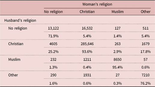
Table 6. General linear mixed model on heterogamy for men and women, including the share of adherents in a region

0 = homogamous marriage; 1 = heterogamous marriage.
Table 7. General linear mixed model on heterogamy for men and women, including religious denomination: full model including the interaction with sex

0 = homogamous marriage; 1 = heterogamous marriage.
In the separate models for men and women, with the exception of ‘dwelling owned’ in men, signs and most significances were the same as in the models including both men and women (Tables 8 and 9 show the models including share of adherents, and Tables 10 and 11 show the models including religious denomination).
Table 8. General linear mixed model on heterogamy for men only including the share of adherents in a region

0 = homogamous marriage, 1 = heterogamous marriage.
Table 9. General linear mixed model on heterogamy for women only including the share of adherents in a region

0 = homogamous marriage, 1 = heterogamous marriage.
Table 10. General linear mixed model on heterogamy for men only, including religious denomination

0 = homogamous marriage, 1 = heterogamous marriage.
Table 11. General linear mixed model on heterogamy for women only, including religious denomination

0 = homogamous marriage, 1 = heterogamous marriage.
Excluding atheists produced comparable results, except that being female was now negatively associated with being in a religious heterogamous marriage in the model including the share of adherents in a region (Table 12). Again, Muslims and adherents of other religions had a higher probability of being in a religious heterogamous marriage than Christians, and Muslim women have the lowest chance of heterogamous marriage (Table 13).
Table 12. General linear mixed model on heterogamy for men and women, including the share of adherents in a region, excluding atheists

0 = homogamous marriage, 1 = heterogamous marriage.
Table 13. General linear mixed model on heterogamy for both men and women, including religious denomination, excluding atheists; full model including the interaction with sex

0 = homogamous marriage, 1 = heterogamous marriage.
Calculating R 2, the overall model explained 25.9% of the variance. Herein, most variance was explained by the share of adherents of a denomination in a region (12.6%), followed by the religious denomination (10.9%), the random factor ‘sample’ (10.7%), education (1.03%), ownership of dwelling (0.95%), age of spouse (0.4%), educational homogamy (0.18%) and sex (0.016%). By analysing men and women separately, a higher proportion of variance was explained by the share of adherents as well as religious denomination in men compared with women (men: 27.6%, women: 4.6%; religious denomination, men: 26.3%, women: 4.4%).
Religious homogamy also predominated when analysing Christians only (Tables 14–16). In addition, in all three models (men and women, women only, men only) a similar pattern was found with regard to signs, and the most significant effects were for age, spouse’s age, education, educational homogamy, owning of a dwelling and the share of adherents to the focal individual’s religion in the couple’s geographical district. Among the Christian denominations, Anglicans, other Christians and Protestants had the highest chance of heterogamous marriage, compared with Catholics, and Orthodox Christians had the lowest chance of being in a heterogamous marriage. Again, the share of adherents to the focal individual’s religion in the couple’s geographical district explained the greatest variance of heterogamous marriage within Christians (~13.7% of the variance explained), albeit without difference between men and women (13.6% vs 13.7% of the variance explained); religious denomination, however, was less important (only 2.3% of the variance explained) (Table 17).
Table 14. Christians only: General linear mixed model on heterogamy for both men and women, including the share of adherents in a region and religious denomination

0 = homogamous marriage, 1 = heterogamous marriage.
Table 15. Christians only: General linear mixed model on heterogamy for men only, including the share of adherents in a region and religious denomination

0 = homogamous marriage, 1 = heterogamous marriage.
Table 16. Christians only: General linear mixed model on heterogamy for women only, including the share of adherents in a region and religious denomination

0 = homogamous marriage, 1 = heterogamous marriage.
Table 17. Variance explained by the different variables in the models including only married Christians

Overall, the expected intermarriage rate (expected heterogamy) was very much higher than the actual intermarriage rate (actual heterogamy). For individuals, the expected intermarriage rate was between 0.86 and almost 1 (in fact 0.99), but the actual intermarriage rate was below 0.8 with a mean of 0.48 (Figure 1a). For Christians (the majority group), the expected intermarriage rate was lower (between 0 and 0.8) but also the actual intermarriage rate was considerable lower (below 0.2 with and mean of 0.044), indicating that it was easy to find a Christian spouse, i.e. a member of the majority group. However, the increase of the actual intermarriage rates indicates that, in the case of more religious and more diverse regions, Christians tended to marry more frequently outside their own community (Figure 1b).

Figure 1. Expected intermarriage rate vs actual intermarriage rate for a) individuals of no religion, b), Christians c) Muslims and d) adherents of other religions.
As Muslims and adherents of ‘other religions’ were a minority population in most of the regions, the expected intermarriage rate was very high (in Muslims between 0.994 and virtually 1 and among adherents of ‘other religions’ between 0.98 and also virtually 1). However, when considering the means, the actual intermarriage rates for Muslims (mean 0.28) and for ‘other religions’ (mean: 0.34) were considerable lower, albeit in some regions the actual intermarriage was higher, and this was caused by the small number of Muslims respectively adherents of ‘other religions’ (<10 individuals) in this regions, i.e. these individuals had a low chance of being engaged in a religious homogamous marriage (Figure 1c, d), and thus married outside their religious communities.
Catholics and Protestants followed a comparable pattern as Christians in general, with an increasing tendency to marry outside their religious communities, following the expected increase in intermarriage rate (Figure 2a). Although Protestants showed a steeper increase in their actual intermarriage rate compared with Catholics, some small groups of Protestants seemed to be strongly engaged in religious homogamy (indicated by the points in the lower right-hand corner of Figure 2b).

Figure 2. Expected intermarriage rate vs actual intermarriage rate for a) Catholics and b) Protestants.
Discussion
In both men and women in the study sample from European countries in 1987–2011, religious heterogamy was found to be more prevalent in atheists than in adherents of any religion. Interestingly, atheists were highly engaged in intermarriage with Christians but not with other denominations, most likely because most atheists originate from a Christian background.
Overall, women in the study had a lower chance of being in a heterogamous marriage than men. This particularly held true for Muslims, where a reasonable proportion of men, but less than 3% of women, were married to Christians. In Christians, in contrast, heterogamy was more prevalent in women than in men. A higher chance of heterogamy in women was also found in the multivariate model controlling for denomination, whereas the opposite was true in the model controlling for share of adherents to an individual’s religion in their area of residence. This change in the sign between models may be attributed to the significant interaction between being a women and religious denomination: Christian women and women of other religious denominations had a higher probability of being in a heterogamous marriage compared with atheists, Christian men and men of other religions. On the other hand, Muslim women had the lowest chance of religious heterogamy. Also, in the model calculated only for women, it is obvious that Muslim women had the lowest probability of being in a heterogamous marriage. The comparably low heterogamy rates of Christian men may be attributed to the large ‘marriage market’ within the Christian community. The data further showed that minority religions faced a higher pressure to marry outside their communities for both men and women – a finding that was predicted by Blau et al. (Reference Blau, Blum and Schwartz1982).
Although in the multivariate models, in addition to sex, several parameters such as age, religious denomination, education and owning of a dwelling significantly affected the chance of being in a religiously heterogamous marriage, the most important factor in terms of variance explained was the share of adherents to an individual’s religion in their area of residence. Accordingly, this fully confirms the work of Thomas (Reference Thomas1951) and Blau et al. (Reference Blau, Blum and Schwartz1982) – that the increase of the share of adherents of a denomination is inversely related to the probability of being in a religious heterogamous marriage. However, by analysing men and women separately, this indicator was of much higher importance for religious intermarriage in men than in women. The same held true also for religious denomination, also explaining a much higher variance in intermarriage in men compared with women.
These findings indicate that, particularly for men, if enough potential mates from the same religious group are available within an area of residence, there seems to be no need for out-marriage. Hence, in the case of large agglomerations of people of the same religious background, the probability of admixture through intermarriage is reduced. Therefore, coinciding with urbanization, the aggregation of larger groups of religiously homogeneous people is likely to reduce intermarriage rates. This effect is higher for men than for women. The data were also in accordance to the data of Beine et al. (Reference Beine, Docquier and Özden2011) concerning the size of a diaspora (i.e. the proportion of migrants of a certain ethnicity and/or religion at a certain place), who showed that the size of the diaspora explains about 71% of the variance of migration to a certain place.
The analysis of the expected intermarriage rate vs the actual intermarriage rate supports this argument, albeit among all religious groups (including individuals with ‘no religion’) the actual intermarriage rate was considerably lower than the expected intermarriage rate. However, if the groups were smaller they tended to practise religious intermarriage more frequently. In particular, members of religious minority groups with a very low number of adherents are forced to marry outside their communities.
While the models indicated that in both men and women, higher education was associated with a higher chance of being in a religiously heterogamous marriage, in terms of variance explained, compared with the size of the diaspora in a certain area, education only played a minor role (~ 1% of the variance), followed by the other explaining factors: educational homogamy, sex, age, and ownership of a dwelling only explained comparably small proportions of the overall variance of religious heterogamy. Nonetheless, the negative estimate of ownership of a dwelling indicates that individuals who had already accumulated some wealth had a lower chance of religious heterogamy compared with those who did not own a dwelling, which also held true if the spouse had the same or a higher education.
For the analysed data, the rates of intermarriage between different religious groups correlated inversely with the size of an individual’s religious group in the area of residence. Yet, by building up genetic ties across religious borders via conjoint offspring, religiously heterogamous couples (albeit of lower fertility; Fieder & Huber, Reference Fieder and Huber2016) foster social cohesion as family members have genetic ties even if ‘separated’ by religion. In such newly formed families co-operation will increase according to Hamilton’s rules of ‘kin selection’, which – in a long-term perspective – may act as a safeguard for social cohesion and peaceful co-existence.
The initial motivation to look at the question of inter-religious marriage stemmed from witnessing the migration flows from mainly Muslim countries (such as Syria, Iraq and Afghanistan) to Europe since 2015. Considering the scope of the migration flows and the potential social impacts, it is necessary to look at intermarriage in addition to the prevailing focus on economic data. Being keenly aware that, while socioeconomic integration is subject to public policy, intermarriage is something that is rightfully beyond this realm and the reported findings of mere observational nature. Also, as diverse religious communities have co-existed in Europe for decades, this is in fact not a matter that is inherently related to migration (therefore it is referred to as social cohesion rather than integration). This leads to a strong argument for the impact of intermarriage when looking at social cohesion in the long run. This would also be in line with the findings of Adams (Reference Adams1983), who asserted that the issue of loyalty towards kin may have practical implications under conditions of warfare (during warfare exogamous women – stemming from the now opposing community – may be faced with contradicting loyalties, while excluding women from warfare might have resolved this antagonism).
At the same time, the analysed data sets (as well as the selection of countries and the dates of the data collection) did not match the initial motivation to study the data. However, the sample size and the diverse nature of countries studied nevertheless provide a pattern that is in line with previous findings and will help to shape future research.
The following restrictions of the analysed data should be taken into consideration. The countries and datasets were selected according to availability of the statistical data (both in terms of country selected and date of data collection). Also, it is evident that marriage is not the only form of cohabitation that is relevant in this context as any form of cohabitation that leads to offspring would support the argument. Furthermore, the issue of premarital conversion by one of the partners (in order to be able to marry) was not addressed, as the census data used did not provide any information on premarital conversion. It is, however, reasonable to assume that the issue of premarital conversion has an impact, which is probably dependent on group size and the degree of religious and/or cultural practice of the respective group. Acknowledging this potential impact on the results, there is no possibility to overcome this potential bias on the basis of cross-sectional census data.
Acknowledgments
The statistical agencies that originally produced the data were the Austria National Bureau of Statistics, Germany, the Federal Statistical Office, Ireland, the Central Statistics Office, Portugal, the National Institute of Statistics, Romania, National Institute of Statistics and the Switzerland Federal Statistical Office.
Funding
There was no funding for this study.
Conflicts of Interest
The authors have no conflicts of interests to declare.
Ethical Approval
The data used were publicly accessible census data provided by IPUMS International (https://international.ipums.org/international/). Ethical approval therefore remains with IPUMS International.


