


Introduction
Submerged active volcanoes in the Southern Ocean are extreme habitats in two ways. First, the water column exhibits consistently cold temperatures and seasonal sea ice cover. Second, extremely high temperature gradients are found around vents and thermal sources. Deception Island is a partially submerged active volcano located in Bransfield Strait, South Shetland Islands. Deception Island has two Antarctic Specially Protected Areas (ASPAs): ASPA 140, which is made up of eleven terrestrial sites, and ASPA 145, which consists of two underwater sub-sites (ATCM 2005a, 2005b). It is one of the most active Antarctic volcanoes today, and home of unique thermophilic plant communities (Smith Reference Smith2005). Geothermal activity is observed in several places, including in Pendulum Cove (Fig. 1) where warm water (~70°C) from hot springs rises to the surface at the shoreline and extends over the sea surface. Three main fault systems cross the island (Rey et al. Reference Rey, Somoza and Martinez-Frias1995), with numerous smaller additional faults in multiple orientations (Maestro et al. Reference Maestro, Somoza, Rey, Martinez-Frias and López-Martinez2007). Long-term seismic studies reveal conspicuous long-period events related to alterations in the shallow hydrothermal system, and volcano-tectonic earthquakes related to regional stresses and local tectonic destabilization induced by volcanic activity (Carmona et al. Reference Carmona, Almendros, Serrano, Stich and Ibañez2012).
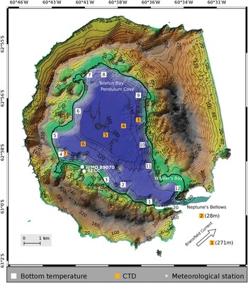
Fig. 1 Detailed map of Deception Island obtained by combining a high-resolution elevation chart (Laboratory of Astronomy, Geodesy and Cartography of the University of Cádiz, Spain) with a high-resolution bathymetry of Port Foster (Spanish Marine Hydrographic Institute). Topographical and bathymetric contours are drawn every 20 m. Conductivity-temperature-depth (CTD) stations are indicated by red squares. Depths of CTD stations 1 and 2 are indicated in parenthesis. Bottom temperature probes are indicated with white squares. Meteorological stations BEGC and WMO-80970 are indicated by white circles. The approximate direction of the Bransfield Current is indicated by a black arrow.
The submerged part of the volcano forms a semi-enclosed bay, known as Port Foster (Fig. 1), of ~6.6×9.6 km in diameter and a maximum depth of ~162 m. After eruptive episodes in 1967, 1969 and 1970, the algae, fungi and bacteria in Port Foster recolonized (Cameron & Benoit Reference Cameron and Benoit1970), and there was repopulation of foraminifera (Finger & Lipps Reference Finger and Lipps1981) and benthic macrofauna (Gallardo & Castillo Reference Gallardo and Castillo1968). Today, the benthic community of Port Foster exhibits low taxonomic richness but high biomass compared to other areas within the South Shetland Islands (Arnaud et al. Reference Arnaud, Lopez, Olaso, Ramil, Ramos-Espla and Ramos1998, Smith et al. Reference Smith, Baldwin, Kaufmann and Sturz2003). Sediment grain size and type, and food resources are the major factors controlling the benthic community structure of Port Foster (Lovell & Trego Reference Lovell and Trego2003). Sediment type shows bathymetrical zonation. Food supplies come from wind-driven and glacier meltwater sediment transport, and from seasonal phytoplankton peaks associated with sea ice retreat. At the bottom of Port Foster, the accumulation of fine grain sediments (mainly ash) from past volcanic activity limits the suspension feeding community (Gray et al. Reference Gray, Sturz, Bruns, Marzan, Dougherty, Law, Brackett and Marcou2003).
The sole communication of Port Foster with Bransfield Strait is through a narrow channel called Neptune’s Bellows (Fig. 1), which is ~550 m wide at its narrowest point and with a sill depth of ~11 m. Port Foster’s hydrography shows strong seasonal variability (Lenn et al. Reference Lenn, Chereskin and Glatts2003). Surface atmospheric warming during summer develops a seasonal thermocline that lasts for approximately six months and breaks in late autumn or early winter due to shear instabilities probably caused by severe wind episodes (Lenn et al. Reference Lenn, Chereskin and Glatts2003). In winter, surface cooling mixes the water column until fully homogeneous, with temperatures near freezing (i.e.~-1.85°C) in late winter. Energy is concentrated at diurnal, semi-diurnal, inertial and fortnightly frequencies (López et al. Reference López, Garcia and Arcilla1994, Lenn et al. Reference Lenn, Chereskin and Glatts2003, Vidal et al. Reference Vidal, Berrocoso and Jigena2011).
In this contribution we use a new dataset collected in January 2012, consisting of conductivity-temperature-depth (CTD) stations inside and outside Port Foster and an array of bottom temperature sensors moored around the bay. Our analysis of these data provide insight into the water mass characteristics and 3D circulation within Port Foster during summer. The bottom temperature array provides us with an excellent opportunity to study the propagation of bottom temperature anomalies around Port Foster.
Data and methods
Hydrographic profiles were measured with a rosette-mounted Seabird 911 CTD profiler on board the Spanish RV Hespérides. Salinity measurements were calibrated on board using a Guildline Autosal Salinometer by standardizing the internal reference against the International Association for the Physical Sciences of the Oceans (IAPSO) standard seawater. A total of seven stations were sampled inside and outside Port Foster (Fig. 1). Two stations were sampled in Bransfield Strait, close to Neptune’s Bellows, on 25 January 2012 from 15h00–16h00 GMT. Five stations were sampled inside Port Foster along an SW–NE section on 25 January 2012 from 17h00–19h00 GMT (low tide during spring; SHN 2012).
Bottom temperatures were measured inside Port Foster using twelve TinyTag Aquatic 2 Gemini dataloggers (model TG-4100; resolution of 0.01°C) lying on the seabed. Prior to deployment, we performed an in situ inter-calibration of all the temperature probes (for details see the supplemental material found at http://dx.doi.org/10.1017/S0954102016000444). The accuracy of the probes was in the order of 0.01°C except for probe 10, which had an accuracy of 0.1°C.
A schematic of the mooring design is shown in Fig. 2. Each mooring consisted of a bottom sensor, 4 kg weight, 6 mm nylon rope and several small buoys to mark the position of the mooring at the sea surface. The length of the rope was ~20–30% longer than the depth of the mooring site to reduce sensor dragging by allowing some wind drifting of the surface buoys.
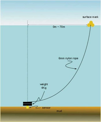
Fig. 2 Schematic of a bottom temperature mooring consisting of a TinyTag temperature sensor, 4 kg weight, 6 mm nylon rope and several small buoys to mark the position of the mooring at the sea surface. In order to reduce sensor dragging by allowing some wind drifting of the surface buoys, the length of the rope was ~20–30% longer than the depth of the mooring site.
Thermistors were programmed to start recording on 4 January 2012 at 23h00 GMT, with one sample per minute. Moorings were deployed around the bay at depths of 18–102 m (Fig. 1, Table I) on 4 January 2012, and were recovered two weeks later on 18 and 19 January 2012. Deployment and recovery operations were performed on board a semi-rigid boat from the Spanish Gabriel de Castilla Antarctic Station.
Table I Location and depth (in m) of the bottom temperature probesFootnote a . The temporal resolution of the sensors was set to 1 min. The sensors were lying on the sea bed.
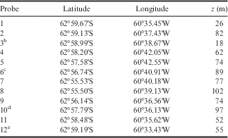
a Location was measured using digital GPS. Approximate depths (z in m) were obtained from a high-resolution bathymetry provided by the Spanish Marine Hydrographic Institute (see Fig. 1).
b Lost probe recovered on 27 January 2012 in Whaler’s Bay.
c Surface buoy recovered at 62°56.700'S, 60°40.776'W, estimated horizontal drift ~130 m.
d Surface buoy recovered at 62°57.803'S, 60°36.053'W, estimated drift ~70 m.
e Surface buoy recovered at 62°59.197’S, 60°33.217'W, estimated drift ~180 m.
Deployment and recovery locations were evaluated by pulling tight on the nylon rope and registered using digital GPS. Eight of the bottom temperature sensors showed no substantial drift (<10 m) with respect to their initial location. Probes 6, 10 and 12 were recovered 130, 70 and 180 m away from their respective deployment sites. Probe 3 was lost and later found on 27 January 2012 at Whaler’s Bay; data from this probe is not used in the present study.
Meteorological data were obtained from two permanent weather stations (locations shown on Fig. 1). BEGC Station is a modular station based on a CR1000 Campbell Scientific data acquisition system, part of a micrometeorological network installed and managed by the University of Extremadura. This station uses an R.M. Young Wind Monitor (model 05103-45, alpine version) at 3 m above ground, which measures wind direction and wind intensity once per minute in summer and every 10 min in winter. For the present study, BEGC summer data has been subsampled to every 10 min. Other measurements include air and soil temperatures, soil thermal flux, relative humidity, global, diffuse and upward solar irradiance, and downward and upward infrared (terrestrial) irradiance. WMO-89070 Station is a Geonica MeteoData MTD3016 station, part of the Antarctic meteorological network installed and managed by the Spanish Agency of Meteorology (AEMET). This station uses an R.M. Young Wind Monitor (model 05106, marine version) at 10 m above ground, which measures wind speed and wind direction once per second and records averaged data at every 10 min. Additional measurements include air temperature, relative humidity, precipitation, global solar radiation and atmospheric pressure.
Sea ice coverage was obtained from LANCE Rapid Response MODIS images (http://lance-modis.eosdis.nasa.gov) and from photographs taken during the Spanish summer campaign at the Gabriel de Castilla Station from 4 December 2011 to 25 January 2012.
Results
Atmospheric conditions and sea ice
Most of Port Foster was covered with sea ice until the first week of December 2011. By the third week of December, only isolated patches were observed at the shore. By the beginning of January 2012 the bay was free of sea ice.
During the experiment, winds in Deception Island were predominantly from the south-west (~240°N) with two episodes of E–SE winds (~100°N) lasting a couple of days (01–03 January and 9–11 January; Fig. 3a & b). Station BEGC recorded a mean speed of 10±5 m s-1 and a maximum speed of 26 m s-1 on 11 January. Wind speed squared is used as a representation of wind stress magnitude. Winds recorded by WMO-89070 were ~30% lower in strength (mean speed: 7±3 ms-1, maximum speed: 19 ms-1) but similar in direction with respect to BEGC (the mean difference between wind direction recorded at the two stations was <0.5°). The differences in wind speed were attributed to the locations of the two weather stations: BEGC is at the top of a hill, whereas WMO-89070 is in the lee of nearby hills (see Fig. 1). The lowest atmospheric pressures were recorded from 11–13 January as a low-pressure system passed over Deception Island (Fig. 3c).
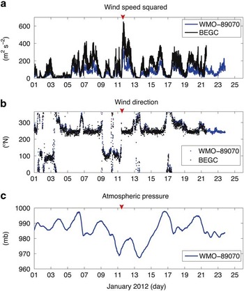
Fig. 3a Wind speed squared (in m2 s-2) and b. wind direction (in °N) from meteorological stations WMO-8970 (in blue) and BEGC (in black). Geographical locations of stations are shown in Fig. 1. c. Atmospheric pressure (in mb). The wind event of 11 January 2012 is indicated by a red arrow.
Hydrography
The water inside Port Foster during our summer survey was Antarctic Surface Water (AASW) with temperatures ranging from ~+1.7°C near the surface to ~-1.5°C at the bottom of the basin (Fig. 4a). The vertical change in salinity over the water column was ~0.15 psu. Water inside Port Foster was substantially more oxygenated than water in Bransfield Strait at all depths (Fig. 4b).

Fig. 4a Potential temperature (θ in °C) – Salinity (S in psu) diagram for the conductivity-temperature-depth (CTD) stations outside (stations 1 and 2) and inside (stations 3 to 7) Port Foster. Geographical locations of stations are shown in Fig. 1. b. Dissolved oxygen (DO in μmol kg-1).
The water column inside Port Foster was divided into two layers separated by a seasonal pycnocline at ~40–60 m (Fig. 5). The upper layer contained relatively warm, fresh and oxygenated water; the lower layer contained colder, saltier, less oxygenated water (Fig. 5a–c). For all variables, horizontal gradients were stronger in the upper layer than in the lower layer. Temperature was highest at the surface of the easternmost station (~1.7°C at station #3).

Fig. 5 Hydrographic section taken across Port Foster using the conductivity-temperature-depth (CTD) stations 3 to 7 (locations shown in Fig. 1). a. Potential temperature (θ in °C). b. Salinity (in psu). c. Dissolved oxygen (in μmol kg-1). d. Stratification (N 2 in s-2), where N is the Brünt-Väisälä frequency. Potential density (σθ in kg m-3) contours (in grey) are plotted in each panel with isopycnals drawn each 0.01 kg m-3.
Circulation in the upper layer was anticlockwise around the bay, with maximum geostrophic velocities of ~0.1 m s-1 (Fig. 6a). Maximum geostrophic shear was found above the pycnocline (Fig. 6b).

Fig. 6 Hydrographic section taken across Port Foster using the conductivity-temperature-depth (CTD) stations 3 to 7 (locations shown in Fig. 1). a. Cross-section geostrophic velocity. Positive (negative) values correspond to northward (southward) direction. b. Shear squared (in s-2),
 $$Shsq=\left( {{{\partial U} \over {\partial z}}} \right)^{2} {\plus}\left( {{{\partial V} \over {\partial z}}} \right)^{2} $$
, where U and V are the orthogonal horizontal velocities of the flow. c. Richardson number, Ri = N
2
/Shsq, where N is the Brünt-Väisälä frequency. Contours of Ri = 1 and Ri = 10 are plotted as thick and thin black lines, respectively. For reference, potential density (σθ in kg m-3) contours are plotted in each panel with isopycnals drawn each 0.01 kg m-3.
$$Shsq=\left( {{{\partial U} \over {\partial z}}} \right)^{2} {\plus}\left( {{{\partial V} \over {\partial z}}} \right)^{2} $$
, where U and V are the orthogonal horizontal velocities of the flow. c. Richardson number, Ri = N
2
/Shsq, where N is the Brünt-Väisälä frequency. Contours of Ri = 1 and Ri = 10 are plotted as thick and thin black lines, respectively. For reference, potential density (σθ in kg m-3) contours are plotted in each panel with isopycnals drawn each 0.01 kg m-3.
The potential for mixing through shear instability can be estimated using the local Richardson number:
 $$Ri={{N^{2} } \over {\left( {{{\partial U} \over {\partial z}}} \right)^{2} {\plus}\left( {{{\partial V} \over {\partial z}}} \right)^{2} }},$$
where N is the Brünt-Väisälä frequency, and U and V are the orthogonal horizontal velocities of the flow. Values of Ri ≤ 1 and Ri ≤ 10 (Fig. 6c) are found in the upper layer, and also in the lower layer of the water column on the western side of the bay (station 6).
Bottom temperature anomalies
Because the bottom temperature probes were located at different depths (Fig. 1, Table I), temperature anomalies relative to the recorded mean temperature were used for each probe instead of their nominal values. Bottom temperature anomalies fluctuate ~1°C at all stations (Fig. 7). All time series show significant cross-correlations >0.3 with several other time series (Table II). Correlations >0.7 are found among stations located at the entrance to Port Foster (i.e. stations 1, 11 and 12; in black in Fig. 7). Part of this large correlation is attributed to long-term variability, e.g. the positive trend observed in stations 1, 11 and 12 after 14 January. Correlations >0.5 are observed among stations located inside the bay (i.e. stations 4 to 6 and 8 to 10; shown in blue in Fig. 7 and highlighted in Table II). The exception is station 7, which shows lower correlation with other stations inside the bay (shown in grey in Fig. 7 and highlighted in Table II).
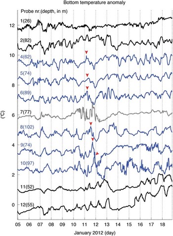
Fig. 7 Bottom temperature anomaly obtained from sensors 1 to 12 located around Port Foster on January 2012. Sensor depths are indicated in parenthesis (in m). Time series are lagged by 1°C for clarity purposes. Geographical locations of the sensors are given in Fig. 1 and Table I. The anomaly observed on 11 January 2012 is indicated by a red arrow. Time series are coloured for highlighting purposes (see text).
Table II Bottom temperature cross-correlations (top) and their time lag (bottom, in h). All correlations are significant (P<0.05).

a Correlations >0.5.
b Cross-correlations of station 7 with other stations inside the bay.
Anomaly peaks propagate, in general, clockwise around Port Foster (Fig. 7). One example is observed on 11 January, when a positive anomaly peak detected at station 4 propagates around the bay towards station 10. It took ~20 h for the perturbation to travel from station 4 to station 10 (i.e. a distance of ~13 km), which leads to a phase speed, c=0.18 m s-1. Considering the period of the perturbation is ~1–2 days (Fig. 7), these values lead to a wavelength λ=c/ω (where c is the phase speed and ω is the wave frequency) of 15–31 km, i.e. of the order of the circumference of the bay (~29 km).
Bottom temperature variability is concentrated at semi-diurnal (~2 cycles per day (cpd)), diurnal (~1 cpd), ~2-day (~0.5 cpd) and larger than ~4-day (~0.25 cpd) periods, according to averaged power spectra (Fig. 8).

Fig. 8 Averaged power spectral density obtained from bottom temperature anomaly time series. Main tidal frequencies (K 1 , O 1 , M 2 and S 2 ) and low-frequency peaks corresponding to two days (2d) and four days (4d) are indicated.
In a Hovmöller diagram (Fig. 9), the propagation of wave-like structures from station 4 to 10 is clear, in particular, early in the record. Correlations between adjacent stations were maxima at time lags of ~1–5 h (with the exception of station 7, Table II). Considering the particular case of stations 4 and 10, the maximum cross-correlation between these two time series was found using a lag of 12.9 h, which leads to a wave phase speed of 0.27 m s-1. Note that this phase speed is 50% larger than that estimated directly from Fig. 7. These differences are attributed to the methodology. The phase speed obtained from the Hovmöller diagram considers the entire time series to estimate the time lag between stations 4 and 10, whereas the phase speed estimated from Fig. 7 (although a more qualitative approach), focuses on the propagation of the anomaly observed on 11–12 June.
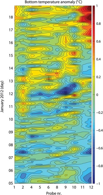
Fig. 9 Hovmöller diagram of bottom temperature anomalies (in °C) obtained inside Port Foster (excluding probe 07). Contours are drawn each 0.1°C. To create this plot, bottom temperature data was smoothed using a 200-point (~3.3 h) moving average.
Discussion
Water masses
The sole water mass inside Port Foster is AASW (Fig. 4). Although there is significant contribution of salinity to stratification, stratification in Port Foster is primarily temperature-forced, in contrast to water in Bransfield Strait where vertical density gradients are mainly due to salinity (Fig. 4a; also see Lenn et al. Reference Lenn, Chereskin and Glatts2003). Winter surface cooling leads to surface-to-bottom near-freezing temperatures during the homogeneous period (Lenn et al. Reference Lenn, Chereskin and Glatts2003 fig. 3), whereas summer surface warming leads to a two-layer system during the stratified season (Fig. 5). The relatively low salinity of the water with respect to Bransfield Strait indicates little local sea ice formation.
Water masses within Port Foster are substantially fresher and more ventilated (higher dissolved oxygen) than water outside the bay in Bransfield Strait (Fig. 4). The relatively high oxygen content of Port Foster with respect to Bransfield Strait suggests that this body of water, although fairly isolated from Bransfield Strait (Lenn et al. Reference Lenn, Chereskin and Glatts2003), is ventilated every winter. Homogeneous conditions lasting several months a year would favour winter cooling full-depth convection and surface-to-bottom oxygen renewal. In the lower layer, elevated oxygen concentrations with respect to those in Bransfield Strait are sustained throughout summer (Fig. 4b). An alternative interpretation for the elevated oxygen content in Port Foster would be a low oxygen utilization rate. However, this seems unlikely given the high biomass found in the bay relative to areas outside (Arnaud et al. Reference Arnaud, Lopez, Olaso, Ramil, Ramos-Espla and Ramos1998, Smith et al. Reference Smith, Baldwin, Kaufmann and Sturz2003). Several studies indicate that elevated dissolved oxygen levels are often related to high phytoplankton activity (e.g. Smith & Piedrahita Reference Smith and Piedrahita1988), in which case Port Foster would be prone to rich aerobic benthic assemblages, with preference for low salinity environments. Long-term (interannual) assemblages would need to survive near-freezing winter temperatures.
Thermal activity modifying surface currents
We interpret the warm, fresh anomaly at the uppermost 30 m of hydrographic station 3 (Fig. 5a & b) to be the result of sea ice melt near the geothermal hot springs of Pendulum Cove. Although the strongest signature of the hot springs is expected to be a low-density anomaly at the surface layer, subsequent mixing with surrounding waters explains the vertical extension of the anomaly down to ~30 m. The vertical extent of the signal is linked to low Ri (Fig. 6c), indicating high mixing inside this water mass. This low-density anomaly from Pendulum Cove modifies the local surface geostrophic circulation at submesoscale (~1 km in the horizontal direction and ~30 m in the vertical direction; Fig. 6a). Although this anomaly may be the signature of a surface eddy or filament, we are unable to determine its complete horizontal extension due to the restrictions of our dataset.
Two-layer circulation and mixing
Geostrophic circulation in the upper layer is anticlockwise around the bay. Data from a long-term mooring close to the location of our bottom temperature station 6 (Fig. 1) from February to November 2000 shows that, at this location, currents at the upper 50 m are primarily towards the south-west (Lenn et al. Reference Lenn, Chereskin and Glatts2003 fig. 7). This suggests that the anticlockwise circulation at the upper layer might be a long-term feature. We postulate that such circulation is due to the sea level gradient across Neptune’s Bellows established by the north-eastward flow of the Bransfield Current, which would cause piling of water towards the north-east wall of the entrance to Port Foster.
Mixing occurs when vertical velocity shear overcomes the stabilizing effect of the buoyancy gradient (Large et al. Reference Large, Mcwilliams and Doney1994). Typically, Richardson numbers <1/4 indicate the potential for mixing through shear instability, although previous studies in Port Foster use Ri ≤ 1 and Ri < 10 to indicate regions where mixing is more likely to occur (e.g. Lenn et al. Reference Lenn, Chereskin and Glatts2003). Shear maxima are found at the base of the mixed layer (Fig. 6b), and the potential for low Richardson numbers is high (therefore mixing is likely) at the upper layer (Fig. 6c).
We interpret the observed temperature fluctuations around the bay (Fig. 7) as vertical movements of the isothermals. Temperature anomalies of ~1°C represent a vertical displacement of ~40 m at the western slope of the basin (Fig. 5a). We postulate that the observed bottom temperature variability is the combination of coastal-trapped waves (CTWs) and internal tides. The CTWs are strictly sub-inertial (i.e. of periods longer than ~13.5 h). They travel in the direction of free-propagating waves, i.e. with shallow water on the left in the Southern Hemisphere. The modelling studies of Stocker & Hutter (Reference Stocker and Hutter1986) show that such waves concentrate towards the shore. Freely propagating internal tides are super-inertial (i.e. of periods shorter than ~13.5 h). Internal wave energy can be scattered in all directions relative to isobaths.
Triggered by wind bursts and tides, CTWs are a ubiquitous phenomenon (Gill & Clarke Reference Gill and Clarke1974). They are hard to observe in nature (Freeland et al. Reference Freeland, Boland, Church, Clarke, Forbes, Huyer, Smith, Thompson and White1986) because it is difficult to isolate them from mesoscale phenomena (~10–100 km). Observing propagation of CTWs requires a relatively closely spaced array of instruments. Stratification, the intensity of the forcing and multiple characteristics of the slope, such as steepness, wavelength of irregularities and bottom friction, determine the amplitude and speed of CTWs (Brink Reference Brink1991, Reference Brink2006). Knowing the local stratification and topographical slope, the cut-off frequency of CTWs inside Port Foster can be determined (see supplemental material found at http://dx.doi.org/10.1017/S0954102016000444). Conditions are suitable for generation of CTWs in Port Foster at sub-inertial periods longer than ~13.5 h during summer and ~15.9 h during winter. Wave-like patterns at periods of ~1–2 days (Figs 7 & 9) are therefore not surprising.
The physical mechanism for the wave forcing is as follows (Brink Reference Brink1991, p. 398). Along-slope wind flows generate cross-slope transport at the surface Ekman layer. To conserve mass, a compensating flow is required at greater depth. When this flow crosses isobaths, vortex stretching/squeezing leads to changes in local relative vorticity, through conservation of potential vorticity. Changes of relative vorticity in along-slope directions give rise to wave propagation.
The most significant sub-inertial (~2-day period) event took place on 11 January. After the strongest wind burst of the time series (south-westerly wind with a maximum speed of ~26 ms-1, Fig. 3), a positive temperature anomaly is observed at station 4, propagating clockwise around the bay (Fig. 7). The physical forcing that triggered the required cross-slope transport on 11 January is, to our best understanding, as follows. From 9–10 January, E–SE winds enter through Neptune’s Bellows and blow roughly parallel to the bathymetric slope at thermistor station 4. To compensate onshore surface Ekman transport, offshore flow is required at greater depth. This causes downwelling of isopycnals, which is observed as an increase in bottom temperature (see 10 January, station 4, Fig. 7). When the wind shifts to south-west (maximum south-west wind of 26 ms-1 on 11 January, Fig. 3), isopycnals rise and bottom temperature decreases (11 January, station 4, Fig. 7).
The isotherm displacement is concurrent with a low-pressure system passing over Port Foster (Fig. 3c). A positive wind stress curl (i.e. positive Ekman pumping) would raise the isopycnals, which would lead to a decrease in bottom temperature. However, the upwelling associated with wind stress curl (Curl z ) is very small. The Ekman pumping velocity (Ek) is given by:
 $$Ek={{Curlz} \over {f\,\rho_0}}={{{{\partial \tau_y} \over {\partial x}}{\minus}{{\partial \tau_x} \over {\partial y}}} \over {f\,\rho_0}},$$
where τx and τy are the zonal and meridional wind stress components, respectively, f is the Coriolis parameter, and ρ 0 is the reference density at the surface. Wind stress data was obtained from ERA-Interim (Simmons et al. Reference Simmons, Uppala, Dee and Kobayashi2007). For our region, f=-2·10-4 s-1, ρ 0 =1000Kgm-3 and Curl z ~ O(10-6) N m-2. These values give an estimated Ek ~ O(1) m day-1, i.e. one order of magnitude smaller than the observed isopycnal displacement. Therefore, we conclude that CTWs excited by the intensified wind rather than wind stress curl explain the pycnocline upwelling on 11 January.
We looked for evidence of CTWs in previous oceanographic studies of Port Foster. An acoustic Doppler profiler coupled to a thermistor chain was deployed from February to November 2000 during the ERUPT Experiment close to the location of our bottom temperature station 6 (Fig. 1) (Smith et al. Reference Smith, Baldwin, Kaufmann and Sturz2003, Site B in their fig. 2). Power spectra obtained from temperature and velocity time series show a low-frequency band at approximately two days (0.02 cph) (Fig. 9 and Lenn et al. Reference Lenn, Chereskin and Glatts2003 fig. 10). In temperature records, low-frequency variability is bottom-trapped during the stratified season and maximum energy is found near the bottom (~151 m; Lenn et al. Reference Lenn, Chereskin and Glatts2003 fig. 10a). Temperature fluctuations are barotropic during the winter homogeneous season. These observations are in agreement with bottom-trapped CTWs. In terms of velocity, near-bottom intensifications were observed in the diurnal band during stratified conditions (Lenn et al. Reference Lenn, Chereskin and Glatts2003 fig. 9a), and at lower frequencies during homogeneous conditions (Lenn et al. Reference Lenn, Chereskin and Glatts2003 fig. 9b). A shift in frequencies could be explained due to stratification (see Eq. A1 found at http://dx.doi.org/10.1017/S0954102016000444).
Propagation of waves at a semi-diurnal frequency, which is slightly super-inertial, can be observed in the western part of the slope (see, for example, probes 04 to 06 on 14–17 January; Figs 7 & 9). Moreover, our Richardson number estimations suggest that mixing is more likely at the western side of the bay (see values of Ri ≤ 1 in the lower layer of the water column, station 6, Fig. 6c). Vidal et al. (Reference Vidal, Berrocoso and Jigena2011) suggest that tidal currents inside Port Foster are very weak, except near Neptune’s Bellows, where they can reach velocities of ~0.64 m s-1 during spring tide (French Reference French1974). However, inside the bay, fluctuations of temperature and salinity are strongly influenced by tidal variability, especially at the semi-diurnal band (Vidal et al. Reference Vidal, Berrocoso and Fernandez-Ros2012). Internal tides could potentially be generated at Neptune’s Bellows sill during each semi-diurnal tide. They would preferentially radiate to the western side of the basin because of exposure. If one traces an energy ray (by drawing a straight line from Neptune’s Bellows as a potential source of energy) to the eastern side of the bay, this ray has to cross over land (over the northern tip of Whaler’s Bay). This means that the eastern side of the bay is a shadow zone for energy radiated from Neptune’s Bellows. This would explain our observations of larger potential for mixing in the western side of the bay. However, this argument does not take into account bathymetric slope and stratification that can refract the internal ray beams around the basin. The best way to look at the role of internal tides inside Port Foster would be with a high-resolution 3D ocean model forced by tides and with realistic hydrography of the bay. If preferential mixing areas inside the bay were confirmed, it would be interesting to place them in context of potential zonation of sediments and/or biological assemblages.
Conclusions
In summer, water in Port Foster is divided into two layers. The upper layer moves anticlockwise around the bay. The lower layer shows instabilities for periods of ~1–2 days that propagate in the direction of free-propagating waves; these are observed in our temperature records as bottom temperature anomalies propagating clockwise around the bay. Strong wind gusts are the probable trigger of such CTWs. Potential for mixing (from Richardson number estimations) appears to be higher on the western side of the bay. We hypothesize that internal tides (which by definition are super-inertial) originating at the sill of Neptune’s Bellows would preferentially radiate towards the western side of the bay, leaving the eastern side in a shadow zone. Surface anomalies caused by sea ice melt and thermal activity modify the local circulation at small (~1 km) scales.
Acknowledgements
We thank Manuel Berrocoso and the Laboratory of Astronomy, Geodesy and Cartography of the University of Cádiz (LAGC, Spain), in particular Amós de Gil and Luis Miguel Peci, for their help in building the temperature moorings and for providing the high-resolution elevation chart of Deception Island. We wish to thank CO Jaime Cervera, officers and crew on board RV Hespérides and CO Enrique Valdés, officers and crew on board RV Las Palmas for their help in making the oceanographic cruises successful. We are grateful to the military personnel at the Gabriel de Castilla Spanish Base for their support in the deployment and recovery of the bottom temperature sensors; the Spanish Marine Hydrographic Institute (IHM), and especially Captain Daniel Gonzalez-Aller and his crew, for providing the high-resolution bathymetry of Port Foster; the Spanish Meteorological Agency (AEMET) for providing the meteorological data from station WMO-89070; and Rafael Benitez for his help with Fig. 1. This work was supported by the Spanish Research and Innovation (I+D+i) Program, through grant numbers CTM2009-08287-E/ANT, CTM2010-09635-E and CTM2011-14056-E, and by the NASA Postdoctoral Program administered by Oak Ridge Associated Universities. This research was carried out at the Jet Propulsion Laboratory, California Institute of Technology, under a contract with NASA. This is a contribution to the ECCO-IcES project funded by the NASA Modeling, Analysis, and Prediction (MAP) programme. We are grateful to two anonymous reviewers and to the editor for their detailed comments that greatly improved the original manuscript. This work is dedicated to Dr Pablo Sangrà Inciarte, outstanding scientist and inspiring teacher.
Author contribution
MAO and MRA designed the moorings. All authors contributed to the data acquisition. MMF and MRA analysed the data. MMF was responsible for writing the manuscript.
Supplementary Material
Supplemental material will be found at http://dx.doi.org/10.1017/S0954102016000444.


