1 Introduction
The global insurance industry is a major economic player, managing ~12% of global financial assets (Swiss Re, 2012). Insurance is also of systemic economic importance, with the failure of an insurer potentially triggering adverse economic and societal impacts. For example, the 2001 collapse of Heath International Holdings Ltd insurance (the second largest insurer in Australia) impacted the wider economy and community events due to the subsequent loss of public liability, professional indemnity and builders warranty insurance (Bellis et al., Reference Bellis, Lyon, Klugman and Shepherd2010).
A key tool to minimise the risk of insurance failure is for insurers to hold capital, commensurate with the risk(s) being undertaken (Australian Prudential Regulatory Authority (APRA), 2012). A key goal of regulation is therefore for insurers to hold sufficient capital to instil confidence and assurance in their ability to meet future liabilities, should unexpected events occur. Various changes to what constitutes “adequate” in terms of capital have occurred over time, and regimes for the determination of capital differ slightly around the world.
This paper examines and compares two such regimes in the context of life insurance. The European-centric Solvency II and Australian-centric Life and General Insurance Capital (LAGIC) capital requirements both adopt a risk-based capital approach which determine capital based on an underlying risk profile, and we apply each to synthetic portfolios of risk and annuity products. This allows a comparison in terms of required capital, and each regime is also compared as to their robustness to a range of relatively severe stress scenarios.
2 Risks, Solvency and Capital
Life insurers face a variety of risks in conducting their business and being able to satisfy promises made to policyholders. We summarise these in Table 1.
Table 1 Risks faced by life insurers.

In the context of such risks, a primary goal of regulatory standards and guidance is to maintain a company’s ability to redeem its liabilities. The associated term of “solvency” can be defined as “the ability of an insurer to meet its liabilities under all contracts at any time” (International Association of Insurance Supervisors, 2015). Concepts like statutory reserves have also historically been adopted, to serve as a provision to meet an insurer’s obligations. Earlier regulatory efforts in Europe to develop an appropriate solvency framework introduced terms such as stabilisation reserves for life insurers, and considered a minimum solvency margin to be a percentage of the technical provisions (Sandstrom, Reference O’Donovan2010).
In 1979, the First Life Directive (79/267/EEC) implemented the requirement for an extra reserve of 4% of the technical provision as a solvency margin (Sandstrom, Reference O’Donovan2010). In 2002, directive 2002/38/EC amended the First Life Directive to form Solvency I. This gave rise to a simple blanket solvency margin based on various percentages of technical provisions for different product types (The European Parliament and the Council of the European Union, 2002).
2.1 Solvency II
Over time, the inadequacies and limitations of Solvency I became apparent. Major issues included the lack of a risk-based approach on both liabilities and assets; a need for better and consistent disclosure to market participants; and good risk management practices and governance were not promoted or given a framework (Central Bank of Ireland, 2013; O’Donovan, Reference Johnson and Mueller2014). As such, a new solvency framework (Solvency II) was established for the European insurance industry. Major objectives were to align capital requirements with underlying risks being faced and as such promote capital adequacy, greater transparency and enhanced supervision. A revised set of capital requirements and risk management standards was established under a three-pillar structure, including quantitative, qualitative and disclosure requirements (The European Parliament and the Council of the European Union, 2009; Society of Actuaries Ireland, Reference Rozar, Rushing and Willeat2013; The European Commission, 2015).
Pillar 1, which we will focus on in this paper, covers the rules relating to the valuation of assets and liabilities, and capital requirements. A supervisory ladder of intervention is embedded into these capital requirements, by setting two target levels of capital: the Minimum Capital Requirement (MCR) and the Solvency Capital Requirement (SCR). The MCR is set so that obligations over the next 12 months are met with a probability of at least 85%, and the SCR is set so that obligations over the next 12 months are met with a probability of at least 99.5%. This establishes an early warning mechanism which provides for early supervisory action when needed. If capital falls below the SCR, this must be restored, but if capital falls below the MCR, “ultimate” supervisory action is triggered. This can involve a range of regulatory actions including liquidation of assets, and transfer of liabilities to other insurers (Jean et al., 2011; European Commission, 2015).
Initial Solvency II preparations began in 2002, with development following a four-level “Lamfalussy” process (named the chair of the creating EU advisory committee). This covered the directive, implementation, supervisory standards and evaluation phases (Comité Européen des Assurances (CEA), 2007). Various political and industry bodies were involved, including the Groupe Consultatif Actuariel Europeen, who represented the European actuarial profession (O’Donovan, Reference Johnson and Mueller2014).
To examine the effect of Solvency II proposals at both company and industry levels, the Committee of European Insurance and Occupational Pensions Supervisors (CEIOPS) launched five quantitative impact studies (QIS) between 2005 and 2011 (CEA, 2007). Amongst other things, these studies highlighted (1) the significant implications of Solvency II including the impact on capital and overall readiness; (2) some inconsistencies between the SCR and MCR; (3) the impact on insurance groups with multiple subsidiaries; (4) qualitative aspects; and (5) consistency with international accounting standards (CEIOPS, 2006 a , 2006 b , 2007, 2008; European Insurance and Occupational Pensions Authority (EIOPA), 2011). Although the final QIS indicated a reduction in surplus capital of ~12% when compared to existing capital requirements, results varied widely depending on the utilisation of an internal model or the standard formula, the size of a company, and the company’s line of business (Jean et al., 2011).
The 2008 global financial crisis (GFC) was a catalyst for reviewing Solvency II development, with more emphasis placed on designing capital rules to prevent a future crisis (Jean et al., 2011). In January 2011, CEIOPS was replaced by the European Insurance and Occupational Pensions Authority (EIOPA), and the Solvency II framework was adapted through a directive called Omnibus II. This enabled EIOPA to enforce binding technical standards as an additional tool for supervision (European Commission, 2013; O’Donovan, Reference Johnson and Mueller2014).
The implementation of Solvency II was delayed from October 2013 to January 2016 (European Commission, 2013) with a key reason for the delay being the approach to long-term liabilities, such as annuities. Omnibus II clarified the treatment of long-term guaranteed products, with measures including a volatility adjustment, a matching adjustment (MA) and the extrapolation of the risk-free interest rate, which helped mitigate the impact of short-term market movements on long-term liabilities (European Commission, 2013). The Omnibus II Directive was approved in March 2014 (European Commission, 2014).
The various phases of Solvency II’s development are summarised in Figure 1.

Figure 1 Solvency II development summary.
2.2 LAGIC
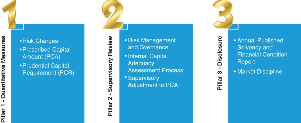
Similarly, Australia’s regulatory regime did not historically incorporate risk-based capital, risk management and disclosure requirements as effectively as they could have. As such, the LAGIC standards were developed, with standards relating to capital requirements developed in light of the GFC and a series of significant natural disasters over the period 2009–2011. Some of the weaknesses of the previous regime in Australia included the lack of allowances for losses from extreme events, the absence of operational risk requirements and the lack of diversification among various risks that life insurers face. LAGIC was implemented on 1 January 2013 (APRA, 2012). LAGIC has strong parallels to Solvency II and also follows a similar 3-pillar structure, as per Figure 2.

We focus on the calculation of the capital requirements for life insurers under pillar 1, which sets out approaches to establish a prescribed capital amount (PCA). The APRA (2012) can apply a “supervisory adjustment” if it considers that the methodology does not produce an appropriate outcome in the particular circumstances of an insurer, which can lead to an increase or decrease in required capital.
3 Synthetic Portfolios and Modelling Assumptions
Three different liability portfolios are used to compare Solvency II and LAGIC. For illustrative purposes in the context of LAGIC requirements, these portfolios are constructed with reference to realistic Australian product and policyholder profiles. However, the adopted portfolios can be adapted to other profiles as needed. The liability portfolios are as follows:
1. a risk portfolio, comprising of 10-year level premium term insurance, and yearly renewable term (YRT) insurance;
2. an annuity portfolio, comprising of life annuities and guaranteed term annuities;
3. a combined portfolio, combining both portfolios above.
All portfolios are assumed to be in run-off, with no new business modelled. This simplifies calculations but more importantly obviates the need to make additional assumptions about volumes of future new business. We calculate capital requirements for the above portfolios under both Solvency II and LAGIC.
3.1 Construction of risk portfolio
The risk portfolio is based on two products, level premium term insurance and YRT insurance. Both risk products only pay the sum insured if the life insured dies, with no savings or traditional insurance aspect to either product, including no surrender value. The level premium term insurance pays out if death occurs within a fixed term, with premiums level for the term of the policy. For the YRT, premiums change each year in line in underlying changes in mortality rates as the life insured ages (Actuaries Institute, 2013).
Each product is assumed to have 10,000 policyholders, representative of the ages and sums insured within the 2004–2008 Financial Services Council (FSC)-KPMG investigation results (FSC, 2012). Average sums insured are inflation-adjusted to obtain 2015 values. in total, 59% of policyholders are male while 41% are female.
An additional assumption is the policy year for level premium term policies, as this impacts the best estimate liability (BEL) calculation, and hence the determination of capital. This is discussed shortly.
The distributions of life insured ages and sum insured for each policy, and the distribution of policy year for level premium term policies, are given in Appendix A.
3.1.1 Premium structure and future expenses
To project future cash flows for risk policies, the pattern and amount of future premiums are required. In line with observed industry pricing, a discount of 5% is applied to the premium for risk policies with sum insured between $500,000 and $1 million, and a discount of 10% is applied to policies with sum insured >$1 million.
Premium rates for YRT policies are based on actual industry quotesFootnote 1 . We did not obtain 10-year level premium term quotes directly, so adopted a cost-plus pricing approach which was based on applying a margin of 20% margin on top of the expected cost of claims and expenses.
Assumptions regarding policy expenses and levels of sales commission were made in consultation with a life insurance actuary currently working in the Australian industry, who confirmed that the assumptions made were not unrealistic. These assumptions are given in Appendix A.
3.2 Construction of annuity portfolio
The annuity portfolio comprises of 10,000 lifetime and 10,000 guaranteed annuity policies. Of all annuity policyholders, 47% are male and 53% are female, which represents the gender mix of the Australian population aged 60 and above.
In a guaranteed annuity, a single premium is paid in exchange for a guaranteed annual payment for a certain duration regardless of whether the policyholder is dead or alive, whereas for a life annuity, a regular annual payment is made if the policyholder is alive. We assume that the duration of payments for a guaranteed annuity follows the life expectancy of the policyholder.
We assume an average annual payment for guaranteed annuities based on the Association of Superannuation Funds of Australia’s (ASFA) (2014) retirement standard for a modest lifestyle, with the average annual payment for guaranteed annuities assumed to be slightly higher than that for life annuities. Based on age bands of 5 years starting at age 60, the average annual annuity payment decreases as age increases to account for the effects of inflation dating back to policy commencement, and greater wealth of more recently retiring annuitants. Surrender values are assumed to be zero and annuity payments are assumed to be level rather than inflation-linked. Appendix B presents the distribution of age and annual annuity payment for males and females, for both annuity products.
Premiums for annuities are not needed for the calculation of liabilities and capital requirements. However, a $50 per policy annual expense to cover administrative costs was allocated to each in force policy for the purposes of liability calculations.
3.3 Combined portfolio
The combined portfolio combines the above risk and annuity portfolios. Therefore, it consists of 40,000 policies, with 10,000 policies each of 10-year level premium term life, YRT, life annuities and guaranteed annuities.
3.4 General modelling assumptions
A range of assumptions in addition to those discussed above are required. For the risk portfolio, all premiums and non-claim expenses are assumed to occur at the beginning of each year, and all claim payments and claim expenses are assumed to occur at the end of each year. For the annuity portfolio, all payments and expenses are assumed to occur at the end of each year.
We ignore the impact of tax on our calculations, preferring to focus on other key drivers of BEL which includes mortality, expenses, lapses, investment returns and discount rates.
Mortality rates for the risk policies are based on an Australian lump sum experience investigation from 2004 to 2008, partitioned by age, gender and smoking status, with a 2-year select period (FSC, 2012). Expected annuitant mortality differs from population mortality due to self-selection effects. However, with small numbers of Australian annuitants and no standard Australian annuitant mortality tables, we refer instead to experience of US individual annuities to determine annuitant mortality as a percentage of Australian population mortality (Australian Bureau of Statistics, 2014). This is given in Appendix C.
Lapse rates are lower for level premium term than for YRT, given the presence of yearly premium increases with YRT. Assumed level premium term insurance lapse rates align closely with lapse rates for US 10-year level premium term insurance (Rozar et al., Reference Mulquiney and Miller2010), and YRT lapse rates are modified from Australian experience (Gilling, 2013) to enable a higher lapse rate in year 1, and higher lapse rates for policyholders aged over 65, due to more significant year-on-year premium increases and less need for cover as the policyholder ages. Assumed lapse rates are given in Appendix C.
Assumptions for both investment returns and discount rates are specific to each portfolio in the context of liability valuation, and are discussed separately below.
3.5 Liabilities and assets for annuities
3.5.1 Liabilities
As part of calculating the BEL for each annuity policy, future net cash outflows at year t are given by:
 $${\rm Net}\,{\rm cash}\,{\rm outflow}\,\left( t \right){\equals}{\rm annual}\,{\rm annuity}\,{\rm payment}{\plus}{\rm expenses}-{\rm investment}\,{\rm income}$$
The net cash outflows are discounted to obtain the value of the BEL for that particular policy. For LAGIC:
 $${\rm Discount}\,{\rm rate}\,{\rm at}\,{\rm duration}\,t{\equals}{\rm risk{\hbox {-}}free}\,{\rm rate}{\plus}{\rm illiquidity}\,{\rm premium}$$
LAGIC prescribes the use of Australian government bond yields as the risk-free rate. Rates up to 10 years were obtained from the Reserve Bank of Australia (RBA) and the June 2015 average forward rates were used. Rates with duration above 10 years were extrapolated using an ultimate forward rate of 6.0% at 60 years duration, an approach adopted by others (Mulquiney & Miller, Reference Jean, Eom and Henriquez2013).
The market interest rates for government bonds incorporate an effective market rate for the liquidity of its securities, known as the liquidity premium. However, the annuity liabilities are not liquid from the insurer or policyholder perspective, hence an illiquidity premium is added to the government bond yield at each duration. The illiquidity premium is calculated as 30% of the A-rated bond spread over the Australian government bonds for durations ≤10 years and 0.2% for durations above 10 years (APRA, 2013 b ).
For Solvency II, we adopt the same risk-free rate as that for LAGIC above. In addition, incentives are given to insurers for matching cash flows of long-term liabilities with those of long-term assetsFootnote 2 . Arising from Omnibus II, this MA aims to offset short-term asset value fluctuations resulting from risks other than default risks by decreasing the BEL, through an increase in the risk-free discount rate. This avoids artificial volatility in technical provisions and capital requirements and means that short-term asset price movements have less impact on the insurer’s ability to meet long-term liabilities.
Hence, we also consider a capital approach which we call Solvency II (MA), which only applies to the annuity and combined portfolios. The relevant discount rate is equal to a risk-free rate plus a MA. The MA is the parallel upward shift to the risk-free discount rate used in valuing eligible policy liabilities, and is equal to (Monetary Authority of Singapore, 2014)
 $${\rm Spread}\,{\rm of}\,{\rm A}{\hbox {-}}{\rm rated}\,{\rm bonds}-{\rm estimated}\,{\rm spread}\,{\rm for}\,{\rm cost}\,{\rm of}\,{\rm default}-{\rm estimated}\,{\rm spread}\,{\rm for}\,\,{\rm cost}\,{\rm of}\,{\rm downgrade}$$
We obtain the estimated spread for cost of default and estimated spread for cost of downgrade from Standard & Poor’s (Reference Sandstrom2015), and the spread of A-rated bonds from the RBA. This gives a MA of 1.47%Footnote 3 , to be applied to annuity valuation under a Solvency II (MA) approach.
3.5.2 Assets
With annuities, a life insurer needs to balance the amount invested in cashflow matched assets such as bonds, and the amount invested in riskier or growth assets, as increasing allocations to growth or non-matched assets will increase capital requirements (and the rate of return on shareholder capital will not necessarily increase). We select an asset portfolio that aligns closely with the annuity asset portfolio of the largest provider of annuities in Australia (Challenger, 2016). This is given in Table 2.
Table 2 Annuity assets portfolio.

This gives rise to an expected investment earning rate of 6% per annum for the annuity portfolio (non-MA).
Under the Solvency II (MA) approach, we assume an asset portfolio of 3% cash and 97% A-rated corporate bonds, with the cash flows of the A-rated bond coupons matched to the expected annuity payments. This gives an assumed investment rate of 5% per annum for the annuity portfolio (MA).
3.6 Liabilities and assets for risk products
3.6.1 Liabilities
For YRT policies, annual premiums tend to increase each year in line with mortality increasing with age. Premiums are set to be higher than the sum of expected claim payments and expenses in the coming year, giving rise to negative policy liabilities. For 10-year level premium term policies, annual premiums are fixed for the 10-year policy term, but claim payments are expected to increase as policyholders get older. This can give rise to a positive BEL which will depend on the age of the policyholder and the policy year. Liabilities are calculated by first calculating the net cash flows in each future year. The net cash flow in year t is
 $${\rm Net}\,{\rm cash}\,{\rm flow}_{t} {\equals}{\rm Premium}_{t} _{{}} -{\rm Expenses}_{t} -{\rm Claims}_{t} {\plus}{\rm Investment}\,{\rm Income}_{t} $$
The BEL is calculated by:
 $$\eqalignno{&{\rm BEL}{\equals}{\minus}\mathop{\sum}\limits_{t{\equals}1} {{{Net\,Cash\,Flows_{t} } \over {\left( {1{\plus}r} \right)^{t}}}} \,\cr &{\rm where}\,r\,{\rm is}\,{\rm the}\,{\rm risk{\minus}free}\,{\rm discount}\,{\rm rate}$$
3.6.2 Assets
Single large claim amounts can occur anytime for risk policies, and a large number of claims can occur if there was a pandemic. Hence, we assume that the assets backing the liabilities (where these are positive, which in this case is only for some level premium term policies) comprise of short-term liquid assets such as cash and A-rated corporate bonds. The asset portfolio backing the liabilities in the risk portfolio is therefore assumed to consist of 91% cash, and 9% corporate bonds. This gives rise to an assumed investment earning rate of 2% per annum for the risk portfolio, which is the recent Australia cash rateFootnote 4 .
4 Applying Solvency II and LAGIC
4.1 Solvency II
We focus on the SCR rather than the MCR. As well as requiring the use of market values wherever possible to value assets and liabilities, Solvency II requires insurers to create technical provisions which correspond to the amount they would pay should they transfer their insurance obligations immediately to another insurer. For this, there are two distinct liability valuation methods. When dealing with hedgeable risksFootnote 5 , the technical provision is the market value. When dealing with non-hedgeable risksFootnote 6 , the technical provision is the best estimate (BE) plus a risk margin. The risk margin is an amount above the BE that an independent third party requires to take over the liabilities, with reference to the cost of capital. The calculation of the risk margin is calculated on each line of business as follows (The European Parliament and the Council of the European Union, 2009):
 $${\rm CoCM}\,{\equals}\,{\rm CoC}{\times}{\raise0.7ex\hbox{${\mathop{\sum}\limits_{t\geq 0} {SCR_{t} } }$} \!\mathord{\left/ {\vphantom {{\mathop{\sum}\limits_{t\geq 0} {SCR_{t} } } {\left( {1{\plus}r_{{t{\plus}1}} } \right)^{{t{\plus}1}} }}}\right.\kern-\nulldelimiterspace}\!\lower0.7ex\hbox{${\left( {1{\plus}r_{{t{\plus}1}} } \right)^{{t{\plus}1}} }$}}$$
where CoCM is the risk margin, CoC the cost of capital rate (assumed as 6%), SCR t the SCR for year t as calculated for the insurer, and r t the risk-free rate for maturity t.
Simplifications for the calculation of the risk margin are allowed, depending on risks involved. We calculate the SCR via a “proportional proxy” approach which approximates the future years’ SCR using a proportionate measure, one of various possible approaches, and selected after consultation with actuaries in the industryFootnote 7 . Essentially, future capital requirements are estimated by multiplying the current year capital requirements by the ratio of expected (discounted) BEL at each future time period to the current year expected (discounted) BEL.
The insurer can use either a standard formula or an internal model to calculate the SCR. The principle behind the standard formula is to reflect as accurately as possible the Value-at-Risk (VaR) of the insurer’s fund at a 99.5% confidence level over a 1-year period (The European Parliament and the Council of the European Union, 2009). The calculation of the SCR is given by
 $${\rm SCR}\,{\equals}\,{\rm BSCR}{\plus}{\rm SCR}_{{{\rm Operational}}} {\plus}{\rm Regulatory}\,{\rm Adjustment}$$
where BSCR is the basic SCRs.
The BSCR incorporates market risk, default risk, intangible risk and life underwriting risk modules. A pre-defined correlation matrix is used to incorporate benefits that arise from any diversification between these risks (The European Parliament and the Council of the European Union, 2009).
 $${\rm BSCR}\,{\equals} \sqrt {\mathop{\sum}\limits_{ij} {{\rm Corr}\,SCR_{{i,j}} {\times}SCR_{i} {\times}SCR_{j} } } {\plus}SCR_{{{\rm Intangible}}} $$
where Corr SCR i,j refers to the pre-defined correlation matrix.
The operational risk charge, SCR Operational, refers to the risk of losses arising from failed or inadequate internal processes, or from external events. It is calculated as:
 $${\rm Min}(0.3{\times}{\rm BSCR},\,{\rm Op}){\plus}0.25{\times}Exp_{{ul}} $$
where Op is the basic operational risk charge for all business = max(Op premiums, Op provisions), Op premiums the 4%×gross earned premiums for life insurance, Op provisions the 0.45%×gross technical provisions for life insurance, Exp ul the annual expenses for unit linked business.
We consider only the capital requirements relating to non-hedgeable risks for our products – for annuities, the longevity and expenses stresses are non-hedgeable; and for risk products, the mortality, catastrophe, lapse and expenses stresses are non-hedgeable. A summary of the applicable market risk stresses and life underwriting risk stresses is given in Appendix D.
4.2 LAGIC
The required level of capital for regulatory purposes is the prudential capital requirement (PCR)Footnote 8 , which is equal to the PCA plus a supervisory adjustment, which is required if APRA “is of the view that there are prudential reasons for doing so” (APRA, 2013 a ). The PCA can be determined by applying a standard method or by using an internal model approved by APRA, or by using a combination of these two. Liabilities under LAGIC are calculated on a BE basis, with risk-free discount rates used in valuing future cash flows. The PCA under the standard method is determined via the components outlined in Table 3.
Table 3 Components of the prescribed capital amount (PCA).

From Table 3 and similar to Solvency II, diversification benefits are accounted for among modules in the insurance risk and asset risk charges, an aggregation benefit which is a diversification benefit between asset risks and insurance risks, and in addition, a combined stress scenario adjustment. A summary of the applicable asset risk charge and insurance risk charge stresses and life underwriting risk stresses is given in Appendix D.
5 Results
Capital requirements for all three portfolios are calculated under Solvency II and LAGIC (see Appendix E for illustrative model points). For Solvency II (MA), capital requirements for the annuity portfolio and the combined portfolio are calculated, as MA only applies to long-term liabilities. We first consider the value of liabilities for each portfolio, under each capital regime. These are given in Table 4:
Table 4 Value of liabilities for each portfolio.

Note: The risk margins are included in Solvency II and Solvency II (matching adjustment (MA)). There is no risk margin under Life and General Insurance Capital (LAGIC) and the liability values displayed in Table 4 are the respective portfolio best estimate liabilities.
Over the entire risk portfolio of YRT and level premium risk policies, the value of liabilities is zeroFootnote 9 as the expected present value of future premiums is greater than the expected present value of future claims and expenses for all YRT policies, and many level premium policies. Hence, there is no net liability over the entire risk portfolio.
For the annuity portfolio, despite the MA of 1.47% being added to the risk-free discount rate when discounting future cash flows under Solvency II (MA), the liability under Solvency II (MA) is greater than Solvency II. This is due to the higher expected investment return rate of 6% under Solvency II compared to 5% under Solvency II (MA), arising from our asset selections under each approach.
5.1 Capital requirements
For convenience, we refer to SCR or PCA as the capital requirement. Table 5 shows these for each portfolio, under each capital regime.
Table 5 Capital requirements.

Note: MA, matching adjustment; LAGIC, Life and General Insurance Capital.
It is a trivial observation that the annuity portfolio requires a substantially larger capital requirement than the risk portfolio. Of more interest are any insights regarding the major contributors to the capital requirements for each portfolio under each capital regime, and also the relationship between the capital requirements for the combined portfolio with the separate risk and annuity portfolios. We therefore break down overall capital requirements into separate risk charge categories. The market risk category in Solvency II is akin to asset risk in LAGIC, and the life underwriting risk category in Solvency II is akin to insurance risk in LAGIC. For convenience, we refer to the nomenclature of Solvency II risk categories. For the risk portfolio, capital requirements are given in Table 6.
Table 6 Risk portfolio capital requirements.

Note: LAGIC, Life and General Insurance Capital.
LAGIC’s capital requirement is 7% higher than Solvency II’s capital requirement for the risk portfolio. Life underwriting risk is the most significant risk category, due to mortality and pandemic risks being two major risks with regards to YRT and level premium term insurance products.
To better analyse the capital requirements for the annuity and combined portfolios, the asset risk category is divided further into its individual modules: equities, properties, interest rate and credit spread. LAGIC has an additional module, inflation rate, which alters the nominal interest rate and affects bonds and the discount rate used in valuing liabilities. For comparison, the LAGIC inflation rate module is combined with the Solvency II interest rate module. Table 7 shows the annuity portfolio capital requirements under Solvency II, Solvency II (MA) and LAGIC.
Table 7 Annuity portfolio capital requirements.

Note: MA, matching adjustment; LAGIC, Life and General Insurance Capital.
Because the market risk modules can significantly affect the market value of the assets in the annuity portfolio, market risk forms the bulk of the capital requirements under Solvency II, Solvency II (MA) and LAGIC. Life underwriting comprises of longevity risk and expense risk, with longevity risk contributing the majority of the capital requirements in this category.
Despite bonds forming 70% of our asset portfolio, and properties and equities forming <30%, the capital requirements related to properties and equities are as large as those related to bonds (interest rate and credit spread). This highlights the magnitude of risk charges that apply to higher-risk assets.
The total capital requirement under Solvency II (MA) is substantially lower than that under Solvency II and LAGIC. This is because the asset portfolio under Solvency II (MA) consists of only corporate bonds and cash, meaning there are no equity and property risk charges. Also, as the assets are ring-fencedFootnote 10 and held to maturity, there is no interest rate risk charge. For the same reason, the credit spread risk charge is also lower.
The stress magnitude for equities is higher in Solvency II (46.5% of market value) when compared to LAGIC (34%), and Solvency II also has a higher operational risk charge. LAGIC has a higher stress on properties than Solvency II (28% of the market value, compared to 25%), higher stresses for credit spread and interest rate (inflation rate included), but also provides for greater diversification benefits due to differences in the pre-defined correlation factors.
The overall result is that Solvency II (MA) yields the lowest capital requirement, with Solvency (II) requirements exceeding those under LAGIC.
As the annuity portfolio’s capital requirements are substantially higher than the risk portfolio’s capital requirements (see Table 5), the capital requirements for the combined portfolio closely mirrors the capital requirements for the annuity portfolio. The distribution of capital requirements among different risk charge categories are very similar to the annuity portfolio.
Importantly, the capital requirement for the combined portfolio is less than the sum of the capital requirements of the annuity and risk portfolio. This is mainly because of the diversification effects between the mortality risks in the risk portfolio and the longevity risks in the annuity portfolio. From the insurer’s perspective, a fall in mortality rates will positively impact the risk portfolio as claims decrease, whilst negatively impacting the annuity portfolio as annuity payments occur for longer, and vice versa.
As a percentage of liabilities, capital requirements are similar for both the annuity and combined portfolios. This is due to the zero BEL for the risk portfolio and the similar capital requirements for the annuity and combined portfolios. Solvency II (MA) has a much lower capital requirement at 6% of liabilities compared to Solvency II (15%) and LAGIC (14%), respectively.
In terms of the overall asset base, we consider the sum of liabilities and capital requirement, as an insurer needs enough assets to provide for liabilities and capital requirements. Table 8 gives the details.
Table 8 Required assets under Solvency II, Solvency II (matching adjustment (MA)) and Life and General Insurance Capital (LAGIC).

Importantly, these figures are the minimum assets required under each regime, in order to be solvent. Insurers will hold additional capital, above and beyond the capital requirements modelled here.
6 Stress Scenarios
Three stress tests/scenarios are applied to all three portfolios, to compare the impact on the sufficiency of the SCR (Solvency II) and the PCR (LAGIC). They are as follows:
1. GFC conditions;
2. pandemic conditions;
3. pandemic + financial crisis conditions.
Such scenarios enable us to better understand the sufficiency of the SCR and PCR under a range of extreme, but nevertheless possible scenarios. We describe each stress scenario below.
6.1 GFC conditions
The 2008 GFC impacted many countries, including Australia. Equity markets fell significantly, with the ASX200 index falling over 50% from its value at the start of 2008. Property prices fell significantly, with the ASX A-REITFootnote 11 index also falling over 50%. The RBA cash rate fell from 7.25% to 3%, and as a result of the “flight-to-quality”Footnote 12 phenomenon, the credit spread for bonds also widened significantly. Indeed, the A-rated corporate bond spread over government bonds increased from an average of 100 basis points in 2007, to 250 basis points at January 2008, to an average of 450 basis points in early 2009Footnote 13 . Based upon this, we select the set of assumptions in Table 9 to model the GFC conditions stress scenario.
Table 9 Global financial crisis conditions stress.

6.2 Pandemic conditions
The 1918 “Spanish” flu pandemic was the most severe pandemic in recent times, with to 3%–5% of the world’s population dying from the virus. In Australia, close to 10,000 people died from a population of around 5 million, translating to an excess additive mortality rate of ~0.2%. Some regions in Europe suffered even more severely, with the excess additive mortality rate in Spain estimated as high as 1% (Johnson & Mueller, Reference Gilling2002).
We consider various excess additive mortality rates due to a pandemic, over a 12-month period. The values of excess additive mortality rates considered are 1%, 0.5%, 0.25% and 0.15%. Solvency II regards 0.15% as a 99.5% worse-case scenario of a pandemic (EIOPA, 2014). It is possible of course that a pandemic may have more adverse effects on certain population cohorts. For example, the 1918 Spanish flu had a greater impact on the young than the elderly (Johnson & Mueller, Reference Gilling2002). Nevertheless, for ease of modelling we assume a constant additive mortality rate for the entire population, an approach not inconsistent with other studies (e.g. APRA, 2007).
6.3 Pandemic and financial crisis conditions
The pandemic scenario above does not incorporate other potential consequences of a pandemic, such as a range of economic impacts. These might include decreased activity in tourism, entertainment, retail and transportation sectors; disrupted business activities arising from involuntary absenteeism from work; and negative investor sentiments (Browne et al., Reference Browne, Bruhn and Huynh2013). Hence, we also consider a stress scenario which combines pandemic and financial impacts, with financial impacts less than for GFC-type conditions, but nevertheless still significant (Table 10).
Table 10 Pandemic + financial crisis stresses.

7 Results of Applying Stress Scenarios
7.1 GFC conditions stress
The GFC stresses are conducted on all portfolios. Results for the risk portfolio are given in Table 11.
Table 11 Global financial crisis conditions stress (risk portfolio).

Note: LAGIC, Life and General Insurance Capital.
The risk portfolio is minimally impacted, as the major risk in this portfolio relates to mortality rather than economic factors. There are few assets compared to the annuity portfolio, and most of these assets are in cash. Although the credit spread stress affects the market value of the A-rated corporate bonds, the impact is significantly lower than the capital requirements.
Next, we consider the annuity and combined portfolios in Tables 12 and 13.
Table 12 Global financial crisis conditions stress (annuity portfolio).

Note: MA, matching adjustment; LAGIC, Life and General Insurance Capital.
Table 13 Global financial crisis conditions stress (combined portfolio).

Note: MA, matching adjustment; LAGIC, Life and General Insurance Capital.
The impact on both portfolios is similar as the assets of the annuity portfolio form the overwhelming majority of the assets in the combined portfolio. In both portfolios, the capital requirements are not sufficient to cover the impact of the GFC conditions stresses under any capital regime, an unsurprising result since the stress amounts are larger than the stresses conducted under the regulatory regimes. However, this does not infer in itself that insolvency would automatically follow for an insurer, as insurers hold capital in excess of the total capital requirements. Furthermore, the 50% fall in equity and property prices conducted in the stress scenario do not happen instantaneously, rather insurers may have time to raise capital or take other actions to manage the risk as it unfolds. Furthermore, our Solvency II and LAGIC capital calculations assumed a regulatory adjustment of zero, which of course may not be realistic in practice.
7.2 Pandemic conditions stress
The pandemic stress scenarios are conducted on all portfolios. For the risk portfolio, the increased mortality rate leads to higher expected claim payments and expenses which worsens the capital position of the insurer. The sufficiency of the capital requirements for the risk portfolio are shown in Table 14.
Table 14 Pandemic conditions stress (risk portfolio).

Note 1:
* The net pandemic stress impact is not the additive pandemic mortality rate multiplied by the sum insured. This is due to the portfolio of yearly renewable term and term policyholders being profit-making before the pandemic stress. The net pandemic stress impact is the expected loss from the entire book of policyholders. Hence, a doubling of rates from 0.25% to 0.5% corresponded to a much higher percentage increase in net pandemic stress impact. This is because the increase from 0.25% to 0.5% did not have a profit to buffer the direct increase in claims compared to an increase from 0% to 0.25%.
Note 2: LAGIC, Life and General Insurance Capital.
For both Solvency II and LAGIC, the capital requirements are not sufficient to cover pandemic cases where the additive mortality is 0.25% or greater. Both capital regimes can accommodate an additive increase to mortality of 0.15%, which is viewed by Solvency II as a 99.5% worst-case pandemic scenario.
A reverse stress test was also conducted to examine the additive mortality rate which would render capital requirements to be insufficient, for each capital regime. This showed that the capital requirements are sufficient for an additive pandemic mortality rate as high as 0.193% and 0.202% for Solvency II and LAGIC, respectively.
The annuity portfolio was not negatively impacted by the pandemic stress scenario, as any rise in population mortality rates decreases the total expected annuity payments. The impact on the combined portfolio is given in Table 15.
Table 15 Pandemic conditions stress (combined portfolio).

Note 1:
* The net exposure amount is the insurance sum insured minus the total current year life annuity payments. It reflects the total exposure to the additional pandemic mortality rate.
Note 2: LAGIC, Life and General Insurance Capital.
The capital requirements are sufficient in covering the pandemic stress impact, although the impact is lower when compared to the risk portfolio. This is due to the natural hedge of mortality risks when holding both death and survival benefits.
7.3 Pandemic and financial crisis conditions stress
In the absence of economic impacts which may arise from a pandemic, the annuity and combined portfolio capital requirements were assessed to be sufficient in the pandemic conditions scenario. Hence, we now assess the sufficiency of the capital requirements for the annuity and combined portfolios in the presence of both pandemic and financial crisis conditions. Tables 16 and 17 give the results for these portfolios.
Table 16 Pandemic and financial crisis conditions stress (annuity portfolio).

Note 1:
* This ratio of [capital requirements] divided by [total stress impact] assesses the extent of sufficiency of the capital requirements. A ratio of larger than 1 indicates sufficient capital requirements.
Note 2: MA, matching adjustment; LAGIC, Life and General Insurance Capital.
Table 17 Pandemic and financial crisis conditions stress (combined portfolio).

Note 1:
* For the risk portfolio component, the expenses stress is calculated as the additional loss incurred by the entire book of policyholders after the increase in expenses are incorporated.
Note 2: MA, matching adjustment; LAGIC, Life and General Insurance Capital.
The stress testing indicates that capital requirements for the annuity and combined portfolios are sufficient for pandemic and financial crisis conditions, under all capital regimes. Overall impact on profit will be negative for an insurer holding an annuity portfolio, even though the higher mortality rates will decrease expected life annuity payments. This is because the financial impact of lower market values for its asset portfolio in the form of higher credit spreads, lower property and lower equity market prices, significantly outweighs the benefits of lower life annuity payments. The stress scenario has a larger impact on the combined portfolio than the annuity portfolio, because the combined portfolio includes the risk portfolio which is severely impacted by the pandemic stress.
In addition, this scenario shows the sufficiency of capital requirements for the annuity and combined portfolios should a less severe market crash occur for reasons not due to a pandemic. Events which led to a 0.5% additive increase to credit spreads and a fall in equity and property prices by 25% have occasionally occurred in recent years, but such scenarios are less severe than the 99.5% worse-case scenario benchmark which Solvency II and LAGIC capital requirements are based on.
8 Conclusion
Solvency II and LAGIC are two examples of improvements on previous capital regimes. Under previous regimes, a fixed proportion of the liabilities are set aside as capital requirements, which may not be ideal as it does not match the underlying profile of risks that an insurer faces. We compare the capital requirements for both Solvency II and LAGIC for three different life insurance portfolios, and then again under three different stress scenarios.
We find that the annuity portfolio has the most significant capital requirements of all three portfolios. It is unsurprising that annuities have higher capital requirements than risk policies, given the significantly higher asset-related risks being faced. With single premium annuities, the insurer has to fulfil a defined set of annuity payments to the policyholder and as such, it carries the risk that the market value of the supporting assets will fall. Longevity risk is also a substantial risk and attracts a significant capital charge. In contrast, for risk insurance, regular premium income is received and is established to be sufficient to provide for future claims, expenses and profit. Its main capital requirements relate to managing a “worse-case scenario” involving mortality risk and catastrophe risk, such as would be evident in a pandemic.
Of additional interest is that the capital requirements for the combined portfolio is less than the sum of the capital requirements of the annuity and risk portfolios, for both Solvency II and LAGIC. This arises from diversification effects between the longevity and mortality risks in the annuity and risk portfolios, respectively.
For the annuity and combined portfolios, Solvency II requires more capital than LAGIC. This is due to higher capital requirements, a higher value of liabilities (technical provisions) arising from the presence of the risk margin, and the absence of the illiquidity premium when compared to LAGIC. However, applying the MA significantly reduces the required capital under Solvency II, as assets held are cash flow matched bonds and cash, with no equities or properties, resulting in lower capital charges. However, there are substantial opportunity costs in this asset strategy as the insurer will not attain higher investment returns that may arise from holding growth assets.
In our stress testing process, the GFC conditions scenario assesses the sufficiency of capital requirements arising from a significant decline in the market value of assets backing the liabilities. This shows that the capital requirements for the annuity and combined portfolio are insufficient for the GFC conditions stress test for both Solvency II and LAGIC, but sufficient under a milder financial crisis. However, there are other impacts of such a scenario which could also be captured with more research. For example, in a severe financial crisis, the ability of policyholders to continue to pay insurance premiums on risk policies may be affected, leading to an increase in policy lapse rates. Additionally, for annuities with surrender values, some annuitants in need of cash may decide to surrender their policy in the event of immediate financial needs.
Under certain levels of pandemic stress, the capital requirements for the risk portfolio are shown to be insufficient for both Solvency II and LAGIC. Additional research could consider pandemic scenarios with greater severity on age groups which form a significant proportion of insured policyholders.
Although we have demonstrated situations in which capital requirements under the different capital regimes may be considered insufficient, for various reasons this does not imply insolvency of the insurer. Insurers hold capital in excess of the capital requirements modelled here, including additional requirements from regulators such as a regulatory adjustment. Furthermore, overall regulatory involvement would likely be dynamic rather than static in a crisis, so that, for example, a regulator would pay close attention to levels of capital to mitigate any activity which could exacerbate any crisis event, such as the forced selling off of assets. This mitigation and raising capital as required may be possible in times of crises, although their plausibility under GFC conditions may be limited.
Additional tools can also reduce the overall risk exposure to such events, such as put options on equity exposure, and stop loss reinsurance as a form of risk transfer. Various product design features also provide a dynamic risk management tool in the event of severe crises, such as the reviewability of YRT premiums, and the flexibility inherent in variable annuities.
Overall, although our stress testing shows that capital requirements may not be sufficient under extreme stress scenarios, the purpose of regimes such as Solvency II and LAGIC is not to guarantee solvency of an insurer under all circumstances. Rather, objectives include ensuring that “under all reasonable circumstances, financial promises made by institutions are met within a stable, efficient and competitive financial system” (APRA, 2012). Indeed, the design of Solvency II and LAGIC capital requirements is to provide capital sufficiency at a level of 99.5% VaR over a 1-year period, equivalent to withstanding a 1 in 200-year event. Therefore, if a pandemic or financial crisis was believed to be a 1 in 400-year event, then it is a sensible observation that the capital requirement designed to withstand a 1 in 200-year event, would prove insufficient of its own accord. Having higher capital requirements than this determined amount may reduce the probability of insolvency, but the cost of holding large amounts of capital is ultimately be borne by policyholders and/or shareholders. Indeed, although capital requirements play a key role in enhancing the solvency of insurers, it is by no means the only approach. It should be complemented by good risk management techniques and appropriate disclosure. These aspects form pillars 2 and 3 of both Solvency II and LAGIC, respectively, and play an equally crucial role in robust insurance regulation.
Acknowledgements
The authors thank Brendan Counsell and Bridget Browne for advice, pointers and contacts provided in bringing this paper together.
Appendix A
Table A.1 Male-level term life insurance age and sum insured (SI) distribution.

Table A.2 Female-level term life insurance age and sum insured (SI) distribution.

Table A.3 Male yearly renewable term life insurance age and sum insured (SI) distribution.

Table A.4 Female yearly renewable term life insurance age and sum insured (SI) distribution.

Table A.5 Level term life insurance policy year distribution.

Table A.6 Expenses for level term and yearly renewable term (YRT) insurance policies.

Table A.7 Commission rates for level term and yearly renewable term (YRT) insurance policies.

Appendix B
Table A.8 Male life annuities age and annual payments distribution.

Table A.9 Female life annuities age and annual payments distribution.

Table A.10 Male guaranteed annuities age and annual payments distribution.

Table A.11 Female guaranteed annuities age and annual payments distribution.

Appendix C

Figure A.1 Annuitant mortality as a percentage of population mortality.
Based on “US annuitant experience” for non-refundable annuities, cited in Berry et al. (Reference Berry, Tsui and Jones2010: 11–12).
Tables A.12 and A.13
Table A.12 Lapse rates for level premium term insurance.

Table A.13 Lapse rates for yearly renewable term insurance.

Appendix D
Table A.14 Summary of Solvency II market risk stresses.

Table A.15 Summary of Solvency II life underwriting risk stresses.

Table A.16 Summary of Life and General Insurance Capital stresses (asset risk charge).

Table A.17 Summary of LAGIC stresses (insurance risk charge).

Appendix E
To illustrate the calculations and workings used when calculating the value of BEL and capital requirements, we select some individual policies (model points) from our portfolios. Projection techniques are then applied in order to determine critical components of Solvency II. Calculations for a 10-year level term life insurance and a life annuity will be showed here.
10-year level premium term insurance
Consider a policy with the following attributes:

Applicable expenses and lapse rates are found in Appendix A. The following tables show the BEL calculation and decrement table, respectively, for this policy.
Table A.18 Best estimate liability (BEL) calculation for a 10-year level term policy.

Table A.19 Decrement table.

Table A.20 Best estimate liability (BEL) calculation for a life annuity policy.

BEL calculation
∙ Premiums (boy) are calculated by multiplying the annual premium by the relevant l x.
∙ Claims (eoy) includes claim amount and claim expenses, with both assumed to occur at end of year. Expected claim amount = sum insured×d x , expected claim expenses =$100×d x .
∙ Expenses (boy) includes commission, initial or renewal expenses (whichever applies) and other expenses.
∙ Interest=interest rate (2%)×(premiums (boy)–expenses (boy)+BEL), if BEL>0.
∙ Net Cash Flow=premium–expenses–claims+interest.
∙ BEL (year 1 end)=[BEL (year 2 end)–Net Cash Flow]÷(1+year 2 Discount Rate).
∙ Policy BEL (year 0)=[BEL (year 1 end)–Net Cash Flow]÷(1+year 1 Discount Rate).
Capital requirements calculations
∙ In calculating the capital requirements for the various modules in Solvency II and LAGIC, assumptions leading to the values in the Tables A.18 and A.19 are changed where appropriate to reflect the relevant stresses of the Solvency II or LAGIC modules.
Life annuity
Consider a female policyholder aged 104 with an annual life annuity payment of $19,859. We will look at the LAGIC case where an illiquidity premium of 0.47% for durations ≤10 years and 0.2% for durations more than 10 years is added to the risk-free discount rate when discounting future cash flows. Table A.20 shows the BEL calculation for this policy.
BEL calculation
∙ Expected payments are assumed to be at the end of the year and are calculated by multiplying Annual Payment by x p Age.
∙ Expenses are assumed to occur at the end of the year and are calculated by multiplying annual expense (taking into account expense inflation) by x p Age.
∙ Interest is calculated by multiplying the interest rate by BEL.
∙ Cash Outflow=Expected Payments+Expenses−Interest.
∙ BEL (year 1 end)=[BEL (year 2 end)+Cash Outflow]÷(1+year 2 Discount Rate).
∙ Policy BEL (year 0)=[BEL (year 1 end)+Cash Outflow]÷(1+year 1 Discount Rate).
Capital requirements calculations
∙ In calculating the capital requirements for the various modules in Solvency II and LAGIC, assumptions leading to the values in the above tables are changed where appropriate to reflect the relevant stresses of the Solvency II or LAGIC modules.