


1 Introduction
The turbulent–non-turbulent interface (TNTI) is the surface that separates the turbulent and irrotational flow regions, which can be commonly observed in free shear layer and boundary layer flows (Corrsin & Kistler Reference Corrsin and Kistler1955; Sreenivasan Reference Sreenivasan1991; Westerweel et al. Reference Westerweel, Fukushima, Pedersen and Hunt2005, Reference Westerweel, Fukushima, Pedersen and Hunt2009; da Silva & Taveira Reference da Silva and Taveira2010; da Silva & dos Reis Reference da Silva and dos Reis2011; da Silva et al. Reference da Silva, Hunt, Eames and Westerweel2014). The properties of the TNTI, which is wrinkled over a wide range of scales in high-Reynolds-number turbulent flows, are crucial in understanding the entrainment and mixing processes (Sreenivasan, Ramshankar & Meneveau Reference Sreenivasan, Ramshankar and Meneveau1989). The results of fractal investigations on the TNTI of compressible turbulent boundary layers can be applied to estimate the surface area, and thus shed light on its multiscale characteristics and improve our knowledge of the entrainment mechanism on the interfaces of compressible turbulent flows.
Since the perspective introduced by Mandelbrot & Pignoni (Reference Mandelbrot and Pignoni1983) that surfaces in flows might present scale-invariant features, a series of experimental studies have been done on corrugated surfaces such as cloud boundaries (Lovejoy Reference Lovejoy1982; Rys & Waldvogel Reference Rys and Waldvogel1986), turbulent flame boundaries (Gouldin Reference Gouldin1987; North & Santavicca Reference North and Santavicca1990), smoke plume boundaries (Praskovsky et al. Reference Praskovsky, Dabberdt, Praskovskaya, Hoydysh and Holynskyj1996) and TNTI in shear flows (Sreenivasan & Meneveau Reference Sreenivasan and Meneveau1986; Constantin, Procaccia & Sreenivasan Reference Constantin, Procaccia and Sreenivasan1991; Catrakis Reference Catrakis2000; de Silva et al. Reference de Silva, Philip, Chauhan, Meneveau and Marusic2013). These experiments reveal the fractal nature of such surfaces and conclude that their fractal dimensions range from 2.3 to 2.4. The fractal dimension of surfaces in fully turbulent flows obtained by theoretical analysis, which is based on the flux of transportable properties across surfaces, also coincides with the experimental results (Sreenivasan et al. Reference Sreenivasan, Ramshankar and Meneveau1989; Meneveau & Sreenivasan Reference Meneveau and Sreenivasan1990).
Although the above assertions appear to be comprehensive, all the TNTI-related researches are based on incompressible flows (Sreenivasan & Meneveau Reference Sreenivasan and Meneveau1986; Constantin et al. Reference Constantin, Procaccia and Sreenivasan1991; Catrakis Reference Catrakis2000; Westerweel et al. Reference Westerweel, Fukushima, Pedersen and Hunt2005, Reference Westerweel, Fukushima, Pedersen and Hunt2009; da Silva & Taveira Reference da Silva and Taveira2010; de Silva et al. Reference de Silva, Philip, Chauhan, Meneveau and Marusic2013), which means that the fractal features of the TNTI of compressible boundary layers is still unknown. Would the TNTI in compressible flows, and even in supersonic flows, obey the same power law? One recent experimental study claims that the box dimension of the TNTI of a Mach-2.95 turbulent boundary layer is 1.53, which implies a fractal dimension of 2.53 (Wang & Wang Reference Wang and Wang2016) and contradicts the present conclusion acquired for incompressible situations. Moreover, the previous experimental studies on the TNTI fractal properties rely on the additive law (Mandelbrot & Pignoni Reference Mandelbrot and Pignoni1983), which is a fundamental hypothesis for fractal analysis. Fractal features of three-dimensional objects can be acquired from their one- or two-dimensional sections through this law, which is built on the assumption that the result of fractal analysis on the intersecting planes is orientation invariant. This assumption was validated under jet situations by Prasad & Sreenivasan (Reference Prasad and Sreenivasan1990) and applied to boundary layer flows directly without further verification. This means that the applicability of the additive law to boundary layer flow, which has a steep gradient of parameters and no symmetry axis, has not been verified.
In this study, we perform an experimental investigation on the TNTI of a turbulent supersonic boundary layer flow with
 $M_{\infty }=2.83$
and acquire data on two orthogonal planes with a high-resolution flow visualisation system known as nanoparticle-tracer planar laser scattering (NPLS). The box-counting results show that the TNTI of supersonic turbulent boundary layers is a self-similar fractal with a fractal dimension of 2.31. The comparison of the results of the box-counting algorithm on two orthogonal planes demonstrates that the scaling exponent of the TNTI of turbulent boundary layers is independent of direction, which is coincident with validity of the additive law, when measured in a size range with the large-scale limit not exceeding approximately
$M_{\infty }=2.83$
and acquire data on two orthogonal planes with a high-resolution flow visualisation system known as nanoparticle-tracer planar laser scattering (NPLS). The box-counting results show that the TNTI of supersonic turbulent boundary layers is a self-similar fractal with a fractal dimension of 2.31. The comparison of the results of the box-counting algorithm on two orthogonal planes demonstrates that the scaling exponent of the TNTI of turbulent boundary layers is independent of direction, which is coincident with validity of the additive law, when measured in a size range with the large-scale limit not exceeding approximately
 $0.05\unicode[STIX]{x1D6FF}$
.
$0.05\unicode[STIX]{x1D6FF}$
.
2 Method
2.1 Experimental set-up
A supersonic turbulent boundary layer with high Reynolds number, the parameters of which are summarised in figure 1, is exploited to examine the fractal facets of the TNTI. Meanwhile, the data obtained by de Silva et al. (Reference de Silva, Philip, Chauhan, Meneveau and Marusic2013) are also extracted and exhibited together to compare the TNTI fractal aspects of compressible and incompressible flows. Two orthogonal planes, surfaces A and B, are used to acquire the NPLS images, where A refers to the
 $x$
–
$x$
–
 $y$
plane and B refers to the
$y$
plane and B refers to the
 $x$
–
$x$
–
 $z$
plane. The rationale for examining these two surfaces is that they are the best representatives for the asymmetric features of the boundary layer flow. To resolve the full range of scales, both fields of view A and B are large enough to cover the scale of boundary layer thickness. For surface A, the total projected length in the
$z$
plane. The rationale for examining these two surfaces is that they are the best representatives for the asymmetric features of the boundary layer flow. To resolve the full range of scales, both fields of view A and B are large enough to cover the scale of boundary layer thickness. For surface A, the total projected length in the
 $x$
-direction of the image sequence applied to extract TNTI is larger than
$x$
-direction of the image sequence applied to extract TNTI is larger than
 $100\unicode[STIX]{x1D6FF}$
. Meanwhile, for surface B, the total area of the images taken into account is larger than
$100\unicode[STIX]{x1D6FF}$
. Meanwhile, for surface B, the total area of the images taken into account is larger than
 $100\unicode[STIX]{x1D6FF}^{2}$
.
$100\unicode[STIX]{x1D6FF}^{2}$
.
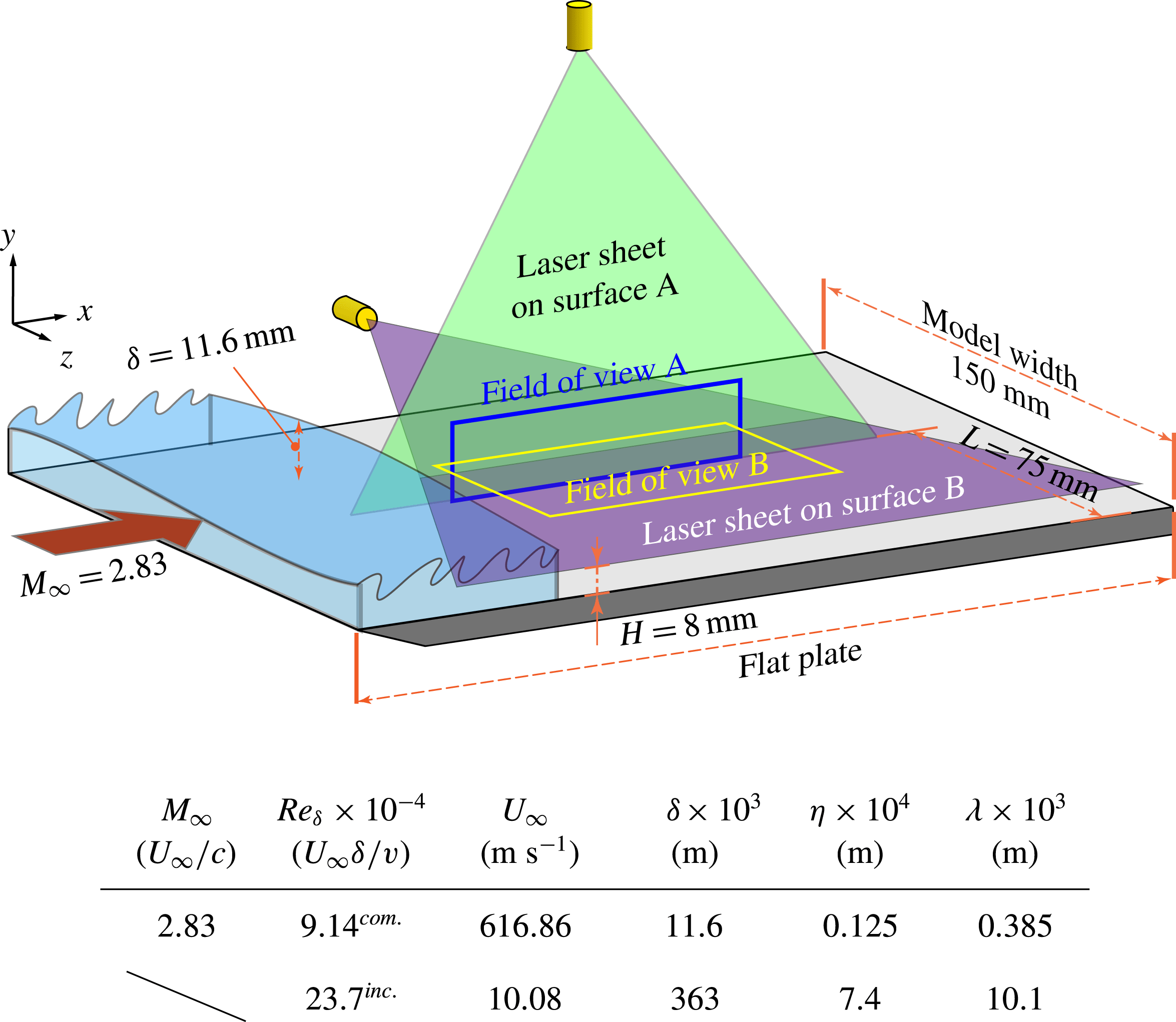
Figure 1. Schematic drawing of the experimental set-up for the NPLS measurements in the Supersonic Wind Tunnel at Nanjing University of Aeronautics and Astronautics, and table of relevant flow properties, where the superscripts com. and inc. refer to the compressible case of the current work and the incompressible case of de Silva et al. (Reference de Silva, Philip, Chauhan, Meneveau and Marusic2013), respectively. The symbols
 $\unicode[STIX]{x1D702}$
and
$\unicode[STIX]{x1D702}$
and
 $\unicode[STIX]{x1D706}$
are the Kolmogorov and Taylor microscales calculated near the interface and
$\unicode[STIX]{x1D706}$
are the Kolmogorov and Taylor microscales calculated near the interface and
 $\unicode[STIX]{x1D6FF}$
is the incoming boundary layer thickness. (The sidewalls are removed in this illustration for clarity.)
$\unicode[STIX]{x1D6FF}$
is the incoming boundary layer thickness. (The sidewalls are removed in this illustration for clarity.)
2.2 Nanoparticle-tracer planar laser scattering (NPLS) visualisation
The NPLS is a nanoparticle-based flow visualisation technique which has been applied successfully to a variety of research on supersonic flows (Bo et al. Reference Bo, Liu, Zhao, Fan and Chao2012; Wang et al. Reference Wang, Xia, Zhao and Wang2013a ,Reference Wang, Wang, Lei and Feng b ; Gang et al. Reference Gang, Yi, Wu and Zhu2014; Tao, Fan & Zhao Reference Tao, Fan and Zhao2014; Zhuang et al. Reference Zhuang, Tan, Liu, Zhang and Ling2017) and is characterised by high spatio-temporal resolution and high signal-to-noise ratio (SNR) (Zhao et al. Reference Zhao, Yi, Tian and Cheng2009). The operating principle and validation of this technique have been demonstrated by Zhao et al. (Reference Zhao, Yi, Tian and Cheng2009).
The camera applied in this study is a digital SLR camera (Canon 1Dx Mark II) with a full-frame sensor of approximately 20.2 megapixels (
 $5472\times 3648$
). The spatial resolutions of the NPLS images of surfaces A and B are 48.0 and
$5472\times 3648$
). The spatial resolutions of the NPLS images of surfaces A and B are 48.0 and
 $74.4~\unicode[STIX]{x03BC}\text{m}~\text{pixel}^{-1}$
, or 3.82 and
$74.4~\unicode[STIX]{x03BC}\text{m}~\text{pixel}^{-1}$
, or 3.82 and
 $5.96~\unicode[STIX]{x1D702}/\text{pixel}$
, respectively. The equivalent spatial resolution of data obtained by de Silva et al. (Reference de Silva, Philip, Chauhan, Meneveau and Marusic2013) is 0.64
$5.96~\unicode[STIX]{x1D702}/\text{pixel}$
, respectively. The equivalent spatial resolution of data obtained by de Silva et al. (Reference de Silva, Philip, Chauhan, Meneveau and Marusic2013) is 0.64
 $\unicode[STIX]{x1D702}/\text{pixel}$
, slightly higher than that of the current experiment. The illumination is provided by a Beamtech Vlite-380 laser (Nd:YAG laser with a wavelength of 532 nm). The pulse duration of this laser is 10 ns – much smaller than the exposure time of the camera. Thus, the actual exposure time of the system is 10 ns, during which the main flow will move approximately
$\unicode[STIX]{x1D702}/\text{pixel}$
, slightly higher than that of the current experiment. The illumination is provided by a Beamtech Vlite-380 laser (Nd:YAG laser with a wavelength of 532 nm). The pulse duration of this laser is 10 ns – much smaller than the exposure time of the camera. Thus, the actual exposure time of the system is 10 ns, during which the main flow will move approximately
 $6~\unicode[STIX]{x03BC}\text{m}$
(a distance much smaller than the spatial resolution of the system, thus causing no motion blur). The application of the NPLS technique provides an available scale range of nearly
$6~\unicode[STIX]{x03BC}\text{m}$
(a distance much smaller than the spatial resolution of the system, thus causing no motion blur). The application of the NPLS technique provides an available scale range of nearly
 $\unicode[STIX]{x1D6FF}/\unicode[STIX]{x1D702}\approx 10^{3}$
and enables the fractal features of TNTI to be examined closely on both scale ends (
$\unicode[STIX]{x1D6FF}/\unicode[STIX]{x1D702}\approx 10^{3}$
and enables the fractal features of TNTI to be examined closely on both scale ends (
 $\unicode[STIX]{x1D6FF}$
level and
$\unicode[STIX]{x1D6FF}$
level and
 $\unicode[STIX]{x1D702}$
level) of the turbulent boundary layer. Such a measurement with a large scale range also enables us to ascertain conclusively if any power-law scaling feature exists.
$\unicode[STIX]{x1D702}$
level) of the turbulent boundary layer. Such a measurement with a large scale range also enables us to ascertain conclusively if any power-law scaling feature exists.
2.3 Turbulent–non-turbulent interface detection
The TNTI of boundary layers can be detected by the method of setting an experiential brightness threshold of greyscale (Prasad & Sreenivasan Reference Prasad and Sreenivasan1989), which has been applied to some TNTI-related investigations (Sreenivasan & Meneveau Reference Sreenivasan and Meneveau1986; Prasad & Sreenivasan Reference Prasad and Sreenivasan1990; Sreenivasan Reference Sreenivasan1991). The brightness threshold in this study is determined on the basis of a hybrid approach of the method of Prasad & Sreenivasan (Reference Prasad and Sreenivasan1990), in which the threshold is acquired by visual inspection, and the method of Prasad & Sreenivasan (Reference Prasad and Sreenivasan1989), in which the threshold is acquired by analysing the histogram of the image. This means the brightness threshold in this study agrees with both the visual inspection and histogram methods simultaneously. According to Prasad & Sreenivasan (Reference Prasad and Sreenivasan1989), when the histogram of the pixel intensity is essentially bimodal, the threshold corresponding to the local minimum is the appropriate one to detect the TNTI. Thus, as is demonstrated in figure 2, 0.27 is selected as the normalised brightness threshold (0 and 1 represent black and white, respectively) applied in the manuscript. No other thresholds are tested in the current research since the fractal dimension of the TNTI is essentially independent of the threshold (Sreenivasan & Meneveau Reference Sreenivasan and Meneveau1986; Prasad & Sreenivasan Reference Prasad and Sreenivasan1990; Sreenivasan Reference Sreenivasan1991; Mathew & Basu Reference Mathew and Basu2002; Westerweel et al. Reference Westerweel, Fukushima, Pedersen and Hunt2009; de Silva et al. Reference de Silva, Philip, Chauhan, Meneveau and Marusic2013), for the reason that the scalar concentration has a large jump across the interface (Westerweel et al. Reference Westerweel, Fukushima, Pedersen and Hunt2009).
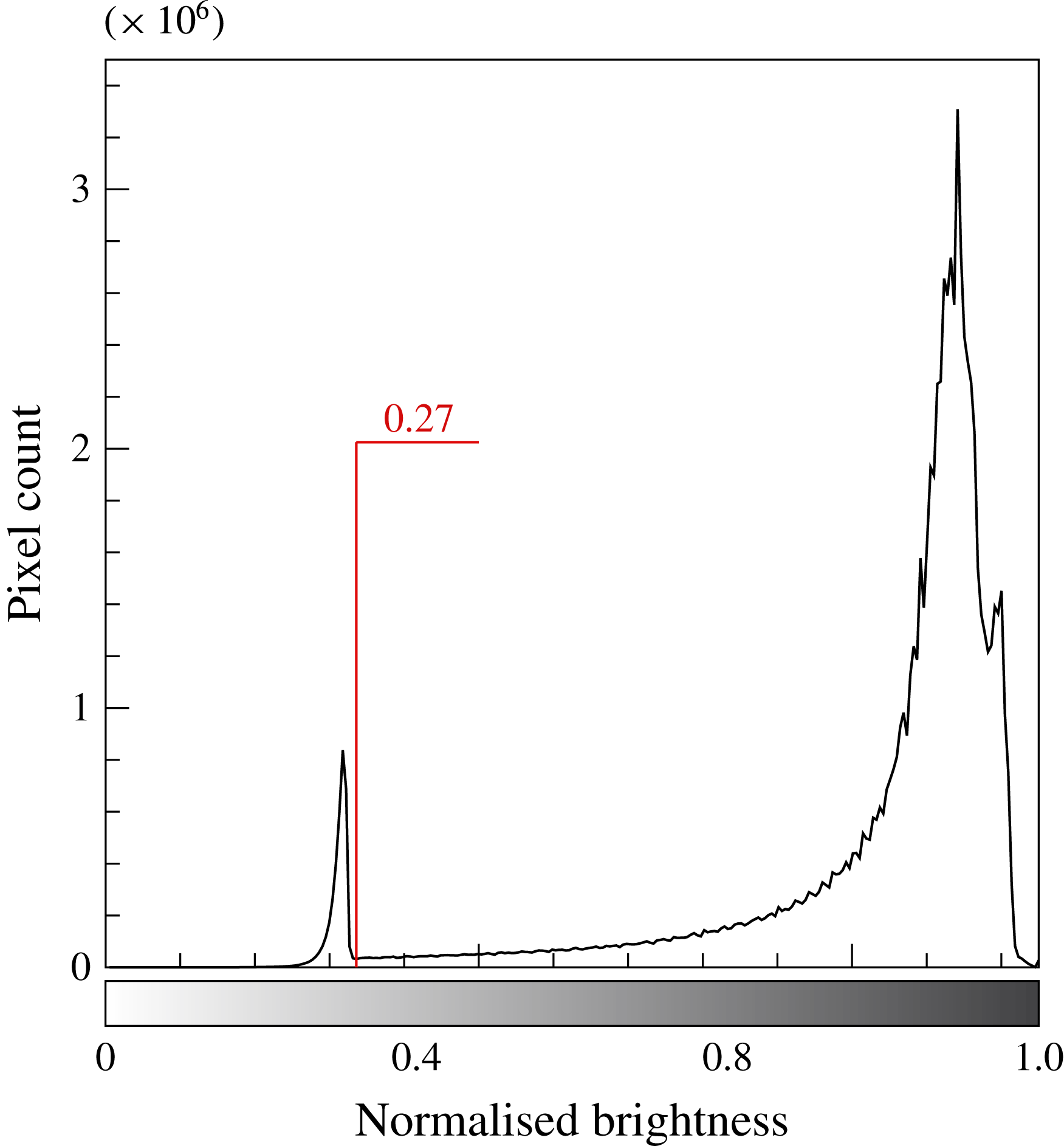
Figure 2. Histogram of normalised brightness calculated from the NPLS images; the bimodal distribution has a local minimum in the vicinity of normalised brightness 0.27.
2.4 Fractal analysis method
Box counting is a method of examining how observations of the detail change with the scale, by breaking the object into pieces, typically ‘box’-shaped, of a series of scale ranges and analysing the pieces at each scale. In this study, we use the box-counting algorithm (Liebovitch & Toth Reference Liebovitch and Toth1989) implemented in the routine FracLac (Karperien, A., FracLac for ImageJ, version 2.5. https://imagej.nih.gov/ij/plugins/fraclac/FLHelp/Introduction.htm. 1999–2013) developed for the ImageJ software package (Schneider, Rasband & Eliceiri Reference Schneider, Rasband and Eliceiri2012) to analyse the fractal character of the TNTI. To be more specific, the box-counting algorithm is applied by calculating
 $N(r)$
, the number of boxes of size
$N(r)$
, the number of boxes of size
 $r$
required to cover the interface, for box sizes ranging from
$r$
required to cover the interface, for box sizes ranging from
 $\unicode[STIX]{x1D702}$
to
$\unicode[STIX]{x1D702}$
to
 $\unicode[STIX]{x1D6FF}$
. Meanwhile, to make the outcome of current study and the result reported by de Silva et al. (Reference de Silva, Philip, Chauhan, Meneveau and Marusic2013) comparable,
$\unicode[STIX]{x1D6FF}$
. Meanwhile, to make the outcome of current study and the result reported by de Silva et al. (Reference de Silva, Philip, Chauhan, Meneveau and Marusic2013) comparable,
 $N(r)$
is normalised by the number of boxes obtained at
$N(r)$
is normalised by the number of boxes obtained at
 $r=0.1\unicode[STIX]{x1D6FF}$
.
$r=0.1\unicode[STIX]{x1D6FF}$
.
3 Results
3.1 Fractal features of TNTI in the supersonic turbulent boundary layer
A fractal analysis on the TNTI detected at surface A is done to investigate the fractal features of TNTI in a supersonic turbulent boundary layer flow. Figure 3(a) shows a sample NPLS image obtained at surface A, along with its partial enlarged view and the corresponding interface. As can be seen, the interface determined is quite realistic, which allows us to examine the fractal features properly. The resulting normalised number of boxes,
 $N(r)_{nor.}$
, is plotted in figure 3(b) using log–log axes. The inset at the top right corner shows the ‘local slope’ acquired by evaluating the logarithmic derivative using the centred finite difference method. It is clear that the two data overlap each other over a wide range, indicating the existence of a power-law scaling feature in the TNTI of the supersonic turbulent boundary layer. The box dimension value of the newly obtained interface in the supersonic case is 1.31, which is the average of the local slope value between the red and aqua vertical dotted lines with a standard error value of 0.007, and the corresponding fractal dimension is 2.31 according to the additive law for intersecting sets. (To compare our data with the existing data, we temporarily assume that the additive law is reliable in the boundary layer flow.) Such results agree well with the previous experimental and theoretical results based on incompressible flows (Sreenivasan & Meneveau Reference Sreenivasan and Meneveau1986; Sreenivasan et al.
Reference Sreenivasan, Ramshankar and Meneveau1989; Meneveau & Sreenivasan Reference Meneveau and Sreenivasan1990; de Silva et al.
Reference de Silva, Philip, Chauhan, Meneveau and Marusic2013). It is observed that the turning points for the compressible and incompressible cases occur at
$N(r)_{nor.}$
, is plotted in figure 3(b) using log–log axes. The inset at the top right corner shows the ‘local slope’ acquired by evaluating the logarithmic derivative using the centred finite difference method. It is clear that the two data overlap each other over a wide range, indicating the existence of a power-law scaling feature in the TNTI of the supersonic turbulent boundary layer. The box dimension value of the newly obtained interface in the supersonic case is 1.31, which is the average of the local slope value between the red and aqua vertical dotted lines with a standard error value of 0.007, and the corresponding fractal dimension is 2.31 according to the additive law for intersecting sets. (To compare our data with the existing data, we temporarily assume that the additive law is reliable in the boundary layer flow.) Such results agree well with the previous experimental and theoretical results based on incompressible flows (Sreenivasan & Meneveau Reference Sreenivasan and Meneveau1986; Sreenivasan et al.
Reference Sreenivasan, Ramshankar and Meneveau1989; Meneveau & Sreenivasan Reference Meneveau and Sreenivasan1990; de Silva et al.
Reference de Silva, Philip, Chauhan, Meneveau and Marusic2013). It is observed that the turning points for the compressible and incompressible cases occur at
 $5\unicode[STIX]{x1D702}^{com.}$
and
$5\unicode[STIX]{x1D702}^{com.}$
and
 $10\unicode[STIX]{x1D702}^{inc.}$
, respectively. Data divergence, caused by the reduced number of boxes counted, occurs near the upper bound for both cases.
$10\unicode[STIX]{x1D702}^{inc.}$
, respectively. Data divergence, caused by the reduced number of boxes counted, occurs near the upper bound for both cases.
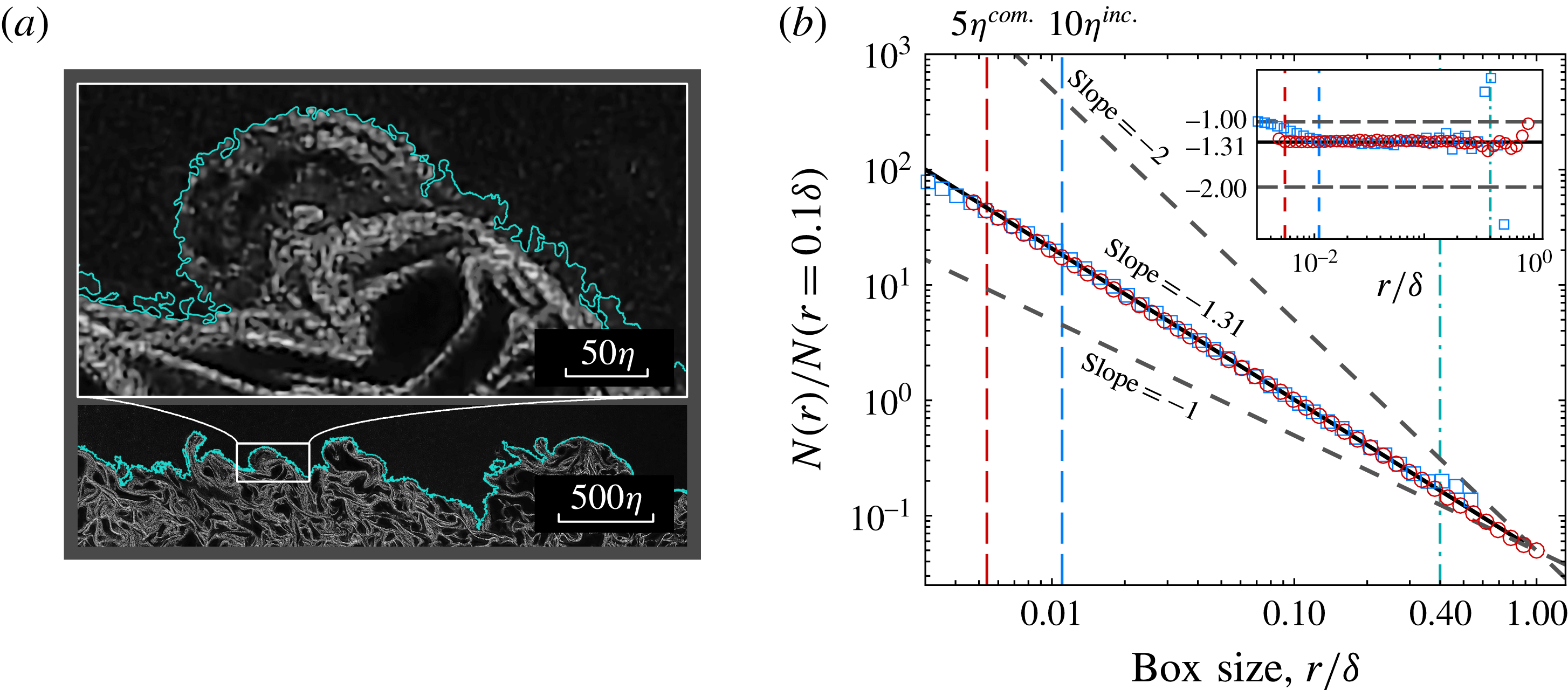
Figure 3. (a) A NPLS image acquired at surface A with its partial enlarged view. The greyscale of the image indicates the concentration of nanoparticles. The solid cyan line indicates the location of the TNTI detected by the threshold method. (b) Log–log plot of the normalised number of square area elements (‘boxes’) of size
 $r$
containing the interface,
$r$
containing the interface,
 $N(r)_{nor.}$
(
$N(r)_{nor.}$
(
 $N(r)_{nor.}=N(r)/N(r=0.1\unicode[STIX]{x1D6FF})$
), versus the box size
$N(r)_{nor.}=N(r)/N(r=0.1\unicode[STIX]{x1D6FF})$
), versus the box size
 $r$
. Circles indicate the compressible case and squares indicate the incompressible case (de Silva et al.
Reference de Silva, Philip, Chauhan, Meneveau and Marusic2013). For comparison purposes, the dashed oblique lines show slopes of
$r$
. Circles indicate the compressible case and squares indicate the incompressible case (de Silva et al.
Reference de Silva, Philip, Chauhan, Meneveau and Marusic2013). For comparison purposes, the dashed oblique lines show slopes of
 $-1$
and
$-1$
and
 $-2$
. Vertical lines show the limits used for each data set.
$-2$
. Vertical lines show the limits used for each data set.
In general, the conclusion obtained here contradicts the results of Wang & Wang (Reference Wang and Wang2016), in which the Canny method, a computational approach to edge detection, is used to detect the TNTI of the supersonic boundary layer. According to Wang & Wang (Reference Wang and Wang2016), a box dimension value of 1.53, which indicates a fractal dimension of 2.53, is obtained at the flat-plate part of the model. Such a distinction might be introduced by the different method applied for interface detection. Actually, the boundaries obtained in their study (Wang & Wang Reference Wang and Wang2016) contain inner structures, thus increasing the level of distortion.
3.2 The applicability of the additive law for the boundary layer flow
A fractal analysis on the TNTI detected at surface B is done to provide direct evidence for the applicability of the additive law for the boundary layer flow. Figure 4(a) exhibits a sample image obtained at surface B with the NPLS technique along with the TNTI identified by the aforementioned method. It is evident that the TNTI acquired at surface B (TNTI-B) is more convoluted than that of surface A (TNTI-A) (figure 3
a), when measured at large scales which are comparable to
 $\unicode[STIX]{x1D6FF}$
. However, when we decrease the order of magnitude of the measurement, the contortion levels of both results become comparable. This implies that the fractal dimensions of TNTI-A and TNTI-B determined at large scales should be different, which breaks the foundation of the additive law – i.e. the isotropic hypothesis. Furthermore, the similarity at small scales shows that the scaling exponent of the TNTI of turbulent boundary layers might be independent of direction.
$\unicode[STIX]{x1D6FF}$
. However, when we decrease the order of magnitude of the measurement, the contortion levels of both results become comparable. This implies that the fractal dimensions of TNTI-A and TNTI-B determined at large scales should be different, which breaks the foundation of the additive law – i.e. the isotropic hypothesis. Furthermore, the similarity at small scales shows that the scaling exponent of the TNTI of turbulent boundary layers might be independent of direction.
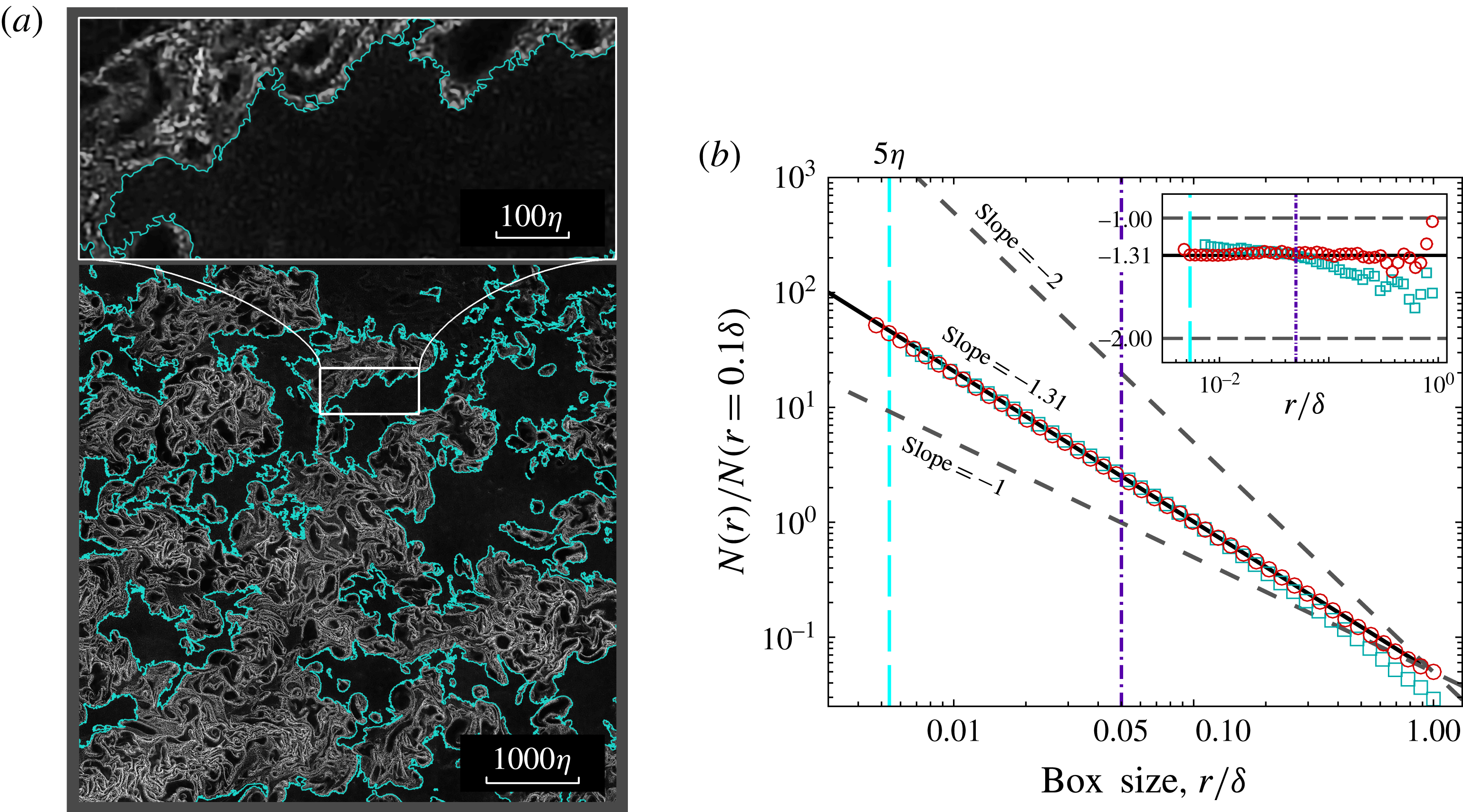
Figure 4. (a) A NPLS image acquired at surface B with its partial enlarged view. The interface detection method is identical to that used for figure 3(a). (b) Plot of the normalised number of boxes needed,
 $N(r)_{nor.}$
, to cover the TNTI at different surfaces. Circles indicate surface A and squares indicate surface B. The inset demonstrates the local slope of these two data sets.
$N(r)_{nor.}$
, to cover the TNTI at different surfaces. Circles indicate surface A and squares indicate surface B. The inset demonstrates the local slope of these two data sets.
The same method as used for TNTI-A is also applied on TNTI-B to obtain its fractal features. The number of boxes required to cover the interface,
 $N(r)$
, is also normalised by the number of boxes obtained at
$N(r)$
, is also normalised by the number of boxes obtained at
 $r=0.1\unicode[STIX]{x1D6FF}$
. The corresponding result is exhibited in figure 4(b) along with the result for TNTI-A. The inset compares the ‘local slope’ of these two data sets. It is clear that these two sets of data are in good agreement when
$r=0.1\unicode[STIX]{x1D6FF}$
. The corresponding result is exhibited in figure 4(b) along with the result for TNTI-A. The inset compares the ‘local slope’ of these two data sets. It is clear that these two sets of data are in good agreement when
 $r$
is smaller than
$r$
is smaller than
 $0.05\unicode[STIX]{x1D6FF}$
. However, the local slope of TNTI-B decreases substantially when
$0.05\unicode[STIX]{x1D6FF}$
. However, the local slope of TNTI-B decreases substantially when
 $r$
is larger than
$r$
is larger than
 $0.05\unicode[STIX]{x1D6FF}$
, exhibiting an obvious difference from that of TNTI-A. This distinction between the tendencies of the two data sets indicates the anisotropy of turbulent structures in the supersonic boundary layer at large scales, and agrees with the finding of Borrell & Jiménez (Reference Borrell and Jiménez2016) that the TNTI of a turbulent boundary layer is not a monofractal. As a result, the isotropic hypothesis cannot be applied to the boundary layer flow for scales beyond
$0.05\unicode[STIX]{x1D6FF}$
, exhibiting an obvious difference from that of TNTI-A. This distinction between the tendencies of the two data sets indicates the anisotropy of turbulent structures in the supersonic boundary layer at large scales, and agrees with the finding of Borrell & Jiménez (Reference Borrell and Jiménez2016) that the TNTI of a turbulent boundary layer is not a monofractal. As a result, the isotropic hypothesis cannot be applied to the boundary layer flow for scales beyond
 $0.05\unicode[STIX]{x1D6FF}$
, which indicates that the additive law is not applicable in scale ranges beyond this certain value for the TNTI of boundary layer flows.
$0.05\unicode[STIX]{x1D6FF}$
, which indicates that the additive law is not applicable in scale ranges beyond this certain value for the TNTI of boundary layer flows.
4 Discussion
While the prior published material for the power-law scaling of the TNTI in supersonic flows is limited and controversial, the results introduced here provide valuable evidence that the TNTI in the supersonic boundary layer flow possesses fractal-like power-law scaling features with
 $D_{f}\approx 2.3{-}2.4$
. A comparison of the fractal features of TNTIs acquired at two orthogonal planes in turbulent boundary flows demonstrates that the scaling exponent is independent of direction, which is consistent with validity of the additive law, when measured in a size range with the large-scale limit not exceeding approximately
$D_{f}\approx 2.3{-}2.4$
. A comparison of the fractal features of TNTIs acquired at two orthogonal planes in turbulent boundary flows demonstrates that the scaling exponent is independent of direction, which is consistent with validity of the additive law, when measured in a size range with the large-scale limit not exceeding approximately
 $0.05\unicode[STIX]{x1D6FF}$
. Such findings are valuable in understanding compressible turbulent boundary layer flows.
$0.05\unicode[STIX]{x1D6FF}$
. Such findings are valuable in understanding compressible turbulent boundary layer flows.
Acknowledgements
This work is funded by the National Natural Science Foundation of China through grant no. 11532007, China Postdoctoral Science Foundation through grant no. 2016M600412 and the Priority Academic Program Development of Jiangsu Higher Education Institutions.


