


1. Introduction
Bistability is a well-known phenomenon in dynamic systems where the system has two equilibrium states and rests in either state. The two states may or may not be connected, as shown in figure 1. For example, the hysteresis phenomenon with one loop, where the solution branches (states) are different when the control parameter is continuously increased and decreased, is a mode of bistable states that are mutually connected (type A in figure 1). In a certain class of problems, the two solution branches are connected through two hysteresis loops (illustrated by the type B of figure 1). Bistability can, however, occur in the absence of hysteresis when the two loops in type B coalesce, creating an isolated solution branch above the continuous branch (illustrated as the type C of figure 1). Since the two solution branches are non-connected, the isolated branch is also denoted as the ‘isola’ branch in the literature (Ganapathisubramanian & Showalter Reference Ganapathisubramanian and Showalter1984; Guidi & Goldbeter Reference Guidi and Goldbeter1997). In such cases, the system can jump from the solution branch of the isola to the continuous branch when the control parameter is varied but cannot undergo the reverse transition regardless of the increase or decrease of control parameter. Transition of this type is referred to as an irreversible transition. The irreversible transition has been found for steady-state bifurcations in chemical and biological systems (e.g. Ganapathisubramanian & Showalter Reference Ganapathisubramanian and Showalter1984; Guidi & Goldbeter Reference Guidi and Goldbeter1997). The bistabilities with hysteresis (types A and B) have also been observed in bluff-body flows, such as vortex-induced vibrations of a circular cylinder (e.g. Feng Reference Feng1968; Khalak & Williamson Reference Khalak and Williamson1999) and oscillatory flow around a near-wall cylinder (e.g. Xiong et al. Reference Xiong, Cheng, Tong and An2018). Nevertheless, irreversible bistable states have rarely been reported, especially in bluff-body flows, to the best knowledge of the authors. The present study provides a detailed account of the irreversible bistable states discovered in two parallel Kármán wakes, in particular on the origins and bifurcation behaviours of the bistable states.

Figure 1. Three types of bistability, namely, type A: bistability with one hysteresis loop, type B: ‘mushroom’ bistability, forming two hysteresis loops and type C: ‘isola’ bistability with irreversible transitions, re-plotted from figure 1 in Guidi & Goldbeter (Reference Guidi and Goldbeter1997). While the horizontal axis,  $\alpha$, is the controlling parameter, the vertical axis,
  $x_s$, represents the response quantity in the system. The limit points, i.e.
  $\alpha _1$–
 $\alpha _4$, are associated with the critical value where the bifurcation occurs. The two equilibrium states are represented by solid lines.
Steady approaching flow around two identical side-by-side cylinders is governed by the gap ratio,  $g^* = G/D$ and Reynolds number,
  $Re = U_\infty D/\nu$, where
  $G$ is the gap distance between two cylinders (as shown in figure 2),
  $U_\infty$ is the approaching velocity,
  $D$ is the cylinder diameter and
  $\nu$ is the kinematic viscosity of the fluid. Many interesting flow features arise due to the interaction of two wakes. For example, at small
  $g^*$ values, e.g.
  $g^* < {\sim }0.4$ in figure 3(a), the flow behaves like a single bluff body with a single Kármán vortex street that forms behind the two cylinders (e.g. the symmetric single bluff-body state, SS, and the asymmetric single bluff-body state, ASS, in figure 3a,c). The characteristic length scale of the flow is of the order of
  $2D$. At large
  $g^*$, individual vortex shedding is formed behind each cylinder and synchronised in-phase and synchronised anti-phase wakes are identified at
  $g^* > {\sim } 1.5$. Corresponding flow characteristics are dominated by length scales of
  ${\sim }D$. At intermediate
  $g^*$ values, e.g.
  $g^* = {\sim }0.4\text {--}1.5$, the flow features are dictated by the interaction of flow characteristics associated with both length scales, leading to complex flow features such as the flip-flop flows, where the flow through the gap flaps laterally at a lower frequency than the vortex shedding frequency.

Figure 2. Computational domain,  $h$-type mesh (the physical mesh) distributions of two side-by-side cylinders at
  $g^{\ast} = 1$ used in the spectral/hp element method. The total mesh resolution is determined by both the distribution of the h-type meshes and the interpolation order
  $N_p$ for the p-type refinement. A close-up view on a
  $hp$-refined mesh consisting of sixth-order Lagrange polynomials
  $(N_{p} = 6)$ on Gauss–Lobatto–Legendre quadrature points is shown in the red-framed inset, where the p-type refined mesh is in grey. Velocity boundary conditions are shown in blue boxes.

Figure 3. Flow regime/mode distributions for the steady flow past (a) two circular cylinders and (b) two square cylinders in a side-by-side arrangement with the variation of gap ratio ( $g^*$) and Reynolds number (
 $Re$) reproduced from (a) Kang (Reference Kang2003), Carini, Giannetti & Auteri (Reference Carini, Giannetti and Auteri2014a) and Carini, Auteri & Giannetti (Reference Carini, Auteri and Giannetti2015) and (b) Mizushima & Hatsuda (Reference Mizushima and Hatsuda2014). The discrete symbols in (a) denote different flow regimes by Kang (Reference Kang2003). The overlapping symbols in regions 1, 2 and 3 in (a) represent cases that are sensitive to different initial conditions. The grey shaded area in (a) is the parameter space occupied by the FF flow by Kang (Reference Kang2003). Corresponding snapshots of the flow states for SS: single bluff-body vortex shedding, ASS: asymmetric bluff-body vortex shedding, IP: in-phase, AP: anti-phase and FF: flip-flop in (a) are represented in (c). The green and purple solid lines in (a) and (b) denoted the neutral curves of IP and AP modes, respectively.
Kang (Reference Kang2003) conducted numerical simulations to map out flow regimes over a parameter space of  $(g^*, Re) = (0.1\text {--}4, 40\text {--}160)$ with relatively coarse
  $Re$ and
  $g^*$ resolutions. Six flow regimes were classified, namely, the anti-phase synchronised (AP), the in-phase synchronised (IP), the flip-flopping (FF), symmetric single bluff body (SS), asymmetric single bluff body (or deflected pattern, ASS) and steady pattern. The flow regime distributions over the parameter space of
  $(g^*, Re) = (0.3\text {--}4, 45\text {--}90)$ are re-plotted in figure 3(a), while the corresponding snapshots of each flow regime are represented in figure 3(c) by means of the present direct numerical simulations (DNS) with zero initial conditions. The FF flow was identified as a dominant flow state in a region at
  $g^* = 0.4\text {--}1.5$, as shown by the grey shaded area in figure 3(a). Kang (Reference Kang2003) also found that the wake patterns in regions 1, 2 and 3 (figure 3a) could bifurcate to the flow states nearby, depending on initial conditions. For instance, the flow state in region 2 can be either FF or IP flow and either IP or AP synchronised state is stable in region 3.
Carini, Giannetti & Auteri (Reference Carini, Giannetti and Auteri2014b) and Carini et al. (Reference Carini, Auteri and Giannetti2015) quantified marginal curves of two distinct FF regions through linear (Floquet) stability analysis of the IP base flow over a parameter space of  $(g^*,Re) = (0.6\text {--}2.4, 51\text {--}70)$. They ascribed the FF flow to an instability of two IP synchronised parallel wakes, rather than the alternative switching between upwards and downwards asymmetric vortex shedding states by Mizushima & Ino (Reference Mizushima and Ino2008) (named the ‘bistability conjecture’ in Carini et al. Reference Carini, Auteri and Giannetti2015). By introducing infinitesimal perturbations on the IP periodic base flow, the Floquet analysis produced a pair of unstable complex-conjugate multipliers above the critical threshold of
  $Re$, leading to a secondary instability of the IP limit cycle. It is also denoted as the Neimark–Sacker bifurcation or the secondary Hopf bifurcation, characterised by a two-dimensional invariant torus bifurcating from the limit cycle in the Poincaré map. By extending the Floquet analysis over the parameter plane, they tracked out two instability regions associated with the Neimark–Sacker bifurcation of the IP vortex shedding cycle, namely FF1 and FF2 regions (as the dotted blue and purple lines overlapped in Kang's regime map in figure 3a). Nevertheless, the DNS carried out by Carini et al. (Reference Carini, Auteri and Giannetti2015) found additional cases with FF features outside the FF1 and FF2 regions, e.g.
  $60 < Re < 65$ at
  $g^* = 1.8$. They speculated that the upper bound of the FF2 curve is associated with a subcritical Neimark–Sacker bifurcation. In addition, after overlapping the flow regime maps obtained through DNS (Kang Reference Kang2003) and the FF1 and FF2 marginal curves by Carini et al. (Reference Carini, Auteri and Giannetti2015), a discrepancy between the FF flow predicted by the two methods is clearly observed. The Floquet analysis of the IP base flow by Carini et al. (Reference Carini, Auteri and Giannetti2015) did not detect the presence of FF flow that was revealed by the DNS (Kang Reference Kang2003) in the vicinity of
  $g^* = 1.5$ (in the region sandwiched between FF1 and FF2 marginal curves). However, the exact cause for the discrepancy is unclear and has not been addressed so far.
Previous studies that may offer some indications for the cause of the above contradiction will be briefly introduced below. By introducing infinitesimal perturbations on the steady symmetric base flow, the linear global stability analysis identified different forms of global instabilities in the steady flow past two circular cylinders (Mizushima & Ino Reference Mizushima and Ino2008; Carini et al. Reference Carini, Giannetti and Auteri2014a) and square cylinders (Mizushima & Hatsuda Reference Mizushima and Hatsuda2014). Two forms of instabilities that relevant to this study are the IP and AP modes, as the green and purple neutral stability curves tracked out over the parameter spaces in figure 3(a,b), respectively. The intersection between IP and AP neutral stability curves are denoted as an IP–AP codimension-two bifurcation point ( $g^*_c$,
  $Re_c$). The IP and AP neutral stability curves separate the parameter space into four regions, as indicated in figure 3(b), which are, region I: the trivial symmetry steady mode; region II: IP mode; region III: AP mode; and region IV: mixed IP–AP mode. The flows in regions II and III are unstable to IP and AP mode disturbances, respectively, and the flow in region IV is unstable to both IP and AP mode disturbances. Region IV can be further divided into IV-1 and IV-2 based on weakly nonlinear analysis, according to a comprehensive study by Mizushima & Hatsuda (Reference Mizushima and Hatsuda2014). The flow is unstable to a mixed mode of IP and AP disturbances of finite amplitudes in region IV-2, while either the IP or AP mode of disturbance will survive by itself in region IV-1, depending on initial conditions. Because unique solutions exist, the flow is independent of initial conditions in regions I, II, III and IV-2. Although the weakly nonlinear analysis by Mizushima & Hatsuda (Reference Mizushima and Hatsuda2014) is for square cylinders, the general findings are expected to be at least qualitatively applicable to the present interest. The bistable feature in region IV-1 is likely relevant to the cause of the discrepancy in predicting FF flows by stability analysis and DNS for two side-by-side circular cylinders. Furthermore, Carini et al. (Reference Carini, Auteri and Giannetti2015), through a weakly nonlinear analysis, speculated that the quasi-periodic features of the FF flow in the vicinity of (
 $g^*_c$,
  $Re_c$) might be associated with the nonlinear interaction between IP and AP states. However, no further investigation has been conducted to address this conjecture.
The objective of the present study is to elucidate the cause for the observed discrepancy in predicting FF flow regimes through DNS by Kang (Reference Kang2003) and stability analysis by Carini et al. (Reference Carini, Auteri and Giannetti2015). The focus of the study is then extended to the bifurcations of the bistable states. The remainder of the paper is organised in the following manner. In § 2, the numerical method and the concepts of phase dynamics are briefly introduced. The bistability phenomenon and the contradiction between DNS and Floquet analysis are explored in § 3. Discussion is offered in § 4. Major conclusions are drawn in § 5. Detailed validations of numerical methods are presented in the appendix.
2. Methodology
2.1. Numerical method
The governing equations for the present DNS are the non-dimensional incompressible Navier–Stokes (N–S) equations
 \begin{equation} \left.\begin{gathered}
\boldsymbol{\nabla}\boldsymbol{\cdot}\boldsymbol{u}=0,\\
\partial\boldsymbol{u}/{\partial
t}={-}(\boldsymbol{u}\boldsymbol{\cdot}\boldsymbol{\nabla})\boldsymbol{u}
-\boldsymbol{\nabla}p+Re^{{-}1}\nabla^2\boldsymbol{u},
\end{gathered}\right\}
\end{equation}
\begin{equation} \left.\begin{gathered}
\boldsymbol{\nabla}\boldsymbol{\cdot}\boldsymbol{u}=0,\\
\partial\boldsymbol{u}/{\partial
t}={-}(\boldsymbol{u}\boldsymbol{\cdot}\boldsymbol{\nabla})\boldsymbol{u}
-\boldsymbol{\nabla}p+Re^{{-}1}\nabla^2\boldsymbol{u},
\end{gathered}\right\}
\end{equation}
where  $\boldsymbol {u} = (u, v)$ is the velocity vector corresponding to
  $\boldsymbol {x} = (x, y)$,
  $t$ is the time and
  $p$ is the pressure.
Equation (2.1) is solved by using a spectral/hp element method embedded in the open-source software package Nektar++ (Cantwell et al. Reference Cantwell2015). The total mesh resolution in the spectral/hp element method is determined by both the distribution of the  $h$-type elements and the interpolation order
  $N_p$ for the
  $p$-type refinement, so that the total mesh equals to
  $N_{el} \times N_p^2$, where
  $N_{el}$ represents the total number of macro-elements in the
  $h$-type mesh. In the present study, sixth-order Lagrange polynomials are used on Gauss–Lobatto–Legendre quadrature points. A second-order time integration method, a velocity correction scheme and a Galerkin formulation are employed for all present simulations. For further information, please refer to the previous studies in Guermond & Shen (Reference Guermond and Shen2003), Blackburn & Sherwin (Reference Blackburn and Sherwin2004), Karniadakis, Israeli & Orszag (Reference Karniadakis, Israeli and Orszag1991) and Vos et al. (Reference Vos, Eskilsson, Bolis, Chun, Kirby and Sherwin2011).
As shown in figure 2, a reference Cartesian coordinate system ( $x$,
$x$,  $y$) is defined with its origin being placed at the mid-point of the line connecting the centres of two cylinders. A rectangular computational domain in the size of
  $(50D + 100D)\times (50D + 50D)$ is adopted for the present scenario, where the steady flow is imposed from left to right in the
  $x$-direction. A Dirichlet velocity boundary condition (
 $u_\infty = U$ and
  $v_\infty = 0$) is specified on the inlet and lateral boundaries of the computational domain sides, while a Neumann velocity boundary condition (
 $\partial u /\partial x = 0$ and
  $\partial v /\partial x = 0$) is implemented on the outlet boundary. A no-slip boundary condition is enforced on the cylinder surfaces. As suggested by Karniadakis et al. (Reference Karniadakis, Israeli and Orszag1991) and Blackburn & Sherwin (Reference Blackburn and Sherwin2004), a high-order Neumann pressure condition is specified on all domain boundaries except a reference zero Dirichlet pressure condition is employed on the outlet boundary.
The initial conditions (IC) specified in the present study include,
(i) zero initial conditions (IC-0);
(ii) non-zero initial conditions: the simulation is initiated with instantaneous flow field from a fully developed flow at the adjacent upper and lower
 $Re$ with an interval of $\Delta Re = 1$, namely IC-$Re_H$ and IC-$Re_L$, respectively;
(iii) non-zero initial conditions: the simulation is initiated with instantaneous flow field from a fully developed flow at the adjacent upper and lower
$g^*$ with an interval of $\Delta g^* = 0.1$, namely IC-$g^*_H$ and IC-$g^*_L$, respectively.


The time-step size  $\Delta t$ for each case is chosen to be
  $\Delta t = 0.002$, based on the Courant–Friedrichs–Lewy (CFL) stability criterion, which is defined as,
 \begin{equation} \textrm{CFL} =\frac{|\boldsymbol{u}|\Delta t}{\Delta l}, \end{equation}
where  $|\boldsymbol {u}|$ is the magnitude of the velocity in each cell and
  $\Delta l$ is the cell size in the direction of the velocity. The maximum value of CFL is kept below 0.5 for all the simulations conducted in the present study.
Detailed two-dimensional (2-D) mesh and numerical scheme validations at  $(g^*, Re) = (1.5, 100)$ will be presented in Appendix A.
2.2. Linear stability analysis
In addition to the 2-D DNS, linear (Floquet) stability analysis is conducted to investigate the bifurcations of periodic base flows in the  $g^*-Re$ space. The Floquet analysis considers the evolution of velocity and pressure perturbations, namely,
  $\boldsymbol {u}'(x, y, t)$ and
  $p'(x, y, t)$, respectively, to a
  $T$-periodic base flow
  $\boldsymbol {U}(x, y, t)$ by solving the linearised N–S equations as,
 \begin{equation} \left.\begin{gathered} \boldsymbol{\nabla}\boldsymbol{\cdot}\boldsymbol{u}'=0,\\ \partial\boldsymbol{u}'/{\partial t}={-}(\boldsymbol{U}\boldsymbol{\cdot}\boldsymbol{\nabla}\boldsymbol{u}' +\boldsymbol{u}'\boldsymbol{\cdot}\boldsymbol{\nabla}\boldsymbol{U})-\boldsymbol{\nabla}p'+Re^{{-}1}\nabla^2\boldsymbol{u}'. \end{gathered}\right\} \end{equation}
Since the perturbed flow  $\boldsymbol {U}+\boldsymbol {u}'$ was recommended to satisfy the same boundary conditions as the base flow
  $\boldsymbol {U}$ (Barkley & Henderson Reference Barkley and Henderson1996), the velocity boundary conditions with
  $\boldsymbol {u}' =0$ and
  $\partial \boldsymbol {u}'/\partial \boldsymbol {n} =0$ are imposed on boundaries where Dirichlet and Neumann conditions are specified for the base flow, respectively. The mesh resolutions are identical to those employed in DNS. The method for 2-D Floquet stability analysis is identical to that reported by Elston, Sheridan & Blackburn (Reference Elston, Sheridan and Blackburn2004) and Elston, Blackburn & Sheridan (Reference Elston, Blackburn and Sheridan2006) and will not be detailed here.
Owing to the periodicity of the base flow  $\boldsymbol {U}(x, y, t)$, a temporal Fourier interpolation method is adopted to reconstruct the base flow through
  $N_{t,s}$ equi-spaced time slices over one period
  $T$. The solutions of
  $\boldsymbol {u}'(x, y, t)$ can be determined by using the Arnoldi method over the
  $K_n$ dimensions of Krylov subspaces and can be written as a sum of components
  $\boldsymbol {u}_{\boldsymbol {i}}'(x, y, t) = \tilde {\boldsymbol {u}}_{\boldsymbol {i}}'(x, y, t) \exp (\lambda T)$, where
  $\tilde {\boldsymbol {u}}_{\boldsymbol {i}}'(x, y, t)$ is a
  $T$-periodic Floquet eigenfunction,
  $\mu = \exp (\lambda T)$ is the Floquet multiplier of the system and
  $\lambda$ is the Floquet exponent. The flow is deemed as unstable if the complex Floquet multiplier
  $\mu$ crosses the unit circle (
 $\lambda > 0$), indicating the perturbation increased exponentially, whereas the flow is stable if
  $\mu$ remains in the unit circle (
 $\lambda < 0$, perturbation decays). As suggested by Elston et al. (Reference Elston, Sheridan and Blackburn2004), the flow is characterised by a secondary period (or quasi-period) when
  $\mu$ is a complex-conjugate pair with
  $\mu =|\mu |\exp (\pm \textrm {i} \omega _s T)$. The secondary period
  $T_s$ of the system is expressed as,
  $T_s = 2{\rm \pi} /\omega _s$.
In this study, two forms of  $T$-periodic base flow, namely, IP base flow, which has a spatio-temporal symmetry, and AP base flow, with a reflection symmetry with respect to the
  $x$-axis, are utilised in the Floquet analysis. The symmetry conditions are listed below,
 $$\begin{gather} \text{IP (spatio-temporal symmetry):} \ \omega_z(x,y,t) ={-}\omega_z(x,-y,t+T/2), \end{gather}$$
 $$\begin{gather}\text{AP (reflection symmetry):} \ \omega_z(x,y,t) ={-}\omega_z(x,-y,t), \end{gather}$$
where the vorticity  $\omega _z(x,y,t)$ indicates the curl of the 2-D velocity components
  $U=(u,v)$,
 \begin{equation} \omega_z= \frac{\partial v}{\partial x}-\frac{\partial u}{\partial y}. \end{equation}
 It is noteworthy that either the IP or AP periodic base flow cannot be simply recovered by using a standard time integration of the governing equations in (2.1) for corresponding  $Re$ where the FF flow develops. Two stabilisation approaches are employed in this study to generate the IP and AP periodic base flows, which will be introduced in Appendix B.
The stability analyses were carried out until the residual of the leading Floquet multiplier reached a value smaller than  $10^{-6}$ or the simulations reached 1000 iterations. The present Floquet analyses on both IP and AP base flows use
  $N_{t,s} = 32$ equi-spaced time slices to reconstruct the base flow feature over
  $T$ and
  $K_n = 16$ dimensions of Krylov subspace iteration are adopted to obtain the Floquet multiplier. Detailed dependence checks for the
  $N_{t,s}$ and
  $K_n$ are presented in Appendix C.
2.3. Phase dynamics
The concept of phase dynamics is routinely used to investigate the dynamics of a self-sustained weakly nonlinear oscillator (or oscillators) subject to periodic external forcing. This method has been applied in the community of fluid mechanics to elucidate the synchronisation behaviours of quasi-periodic phenomena in self-excited jets (Li & Juniper Reference Li and Juniper2013), thermoacoustic systems (Kashinath, Li & Juniper Reference Kashinath, Li and Juniper2018) and bluff-body flows (Ren et al. Reference Ren, Cheng, Tong, Xiong and Chen2019; Konstantinidis et al. Reference Konstantinidis, Zhao, Leontini, Lo Jacono and Sheridan2020; Aswathy & Sarkar Reference Aswathy and Sarkar2021) and demonstrated to be effective in revealing the nature of flows that involves complex interactions.
The global wake structures behind two side-by-side cylinders are similar to a feedback system, where the Kármán vortex street that forms behind one cylinder is influenced by that of the other. The synchronisation state between the two wakes is determined based on the instantaneous phase difference between lifts on the two cylinders as,
 \begin{equation} \varPsi(t) =\varPsi_1(t)-\varPsi_2(t), \end{equation}
where  $\varPsi _i(t)$ represents the instantaneous phase of lift coefficient fluctuation
  $\Delta C_{Li} (t) = C_{Li} (t) - \langle C_{Li} (t)\rangle _{T_a}$ determined from the Hilbert transform (Pikovsky, Rosenblum & Kurths Reference Pikovsky, Rosenblum and Kurths2003),
  $i (= 1$ and
  $2)$ denotes the
  $i$th cylinder and
  $\langle \cdot \rangle _{T_a}$ denotes a time-averaged quantity over the statistical period,
  $T_a$.
Generally, the resulting phase dynamics contains four synchronisation states, namely, phase locking, phase trapping, phase drifting and phase slipping, according to the temporal variations of  $\varPsi (t)$. While the
  $\varPsi (t)$ of the phase locking state is time invariant,
  $\varPsi (t)$ increases or decreases monotonically with time in the phase drifting state. The phase trapping state is featured by a long period oscillation of
  $\varPsi (t)$ around a constant value, while the
  $\varPsi (t)$ in the phase slipping state experiences a sudden slip at the end of each long period of oscillation (epoch). Similar but more detailed discussions can be found elsewhere (Pikovsky et al. Reference Pikovsky, Rosenblum and Kurths2003; Li & Juniper Reference Li and Juniper2013; Ren et al. Reference Ren, Cheng, Tong, Xiong and Chen2019).
In the present study, the value of  $\langle \varPsi \rangle _{T_a}$ is used to interpret the IP or AP synchronisation state for periodic flows as the phase dynamics of those flows is in the phase locking state. For instance, when two wakes are in the IP synchronisation,
  $\langle \varPsi \rangle _{T_a}$ exactly equals to an even-number multiple of
  ${\rm \pi}$, whereas the flow is deemed in the AP synchronisation when
  $\langle \varPsi \rangle _{T_a}$ equals to an odd-number multiple of
  ${\rm \pi}$. All the values of
  $\langle \varPsi \rangle _{T_a}$ are shifted to the interval of
  $[0, {\rm \pi}]$ in the present study to provide a clear view of IP or AP synchronisation of two cylinder wakes.
For the FF flows, a rich phase dynamics, such as phase drifting, phase slipping and phase trapping states, is observed. Since  $\varPsi (t)$ varies typically with time in FF flows, we found that the mean value of
  $\varPsi (t)$ over a statistical period,
  $\langle \varPsi \rangle _{T_a}$ is not a good measure for classifying the synchronisations of FF flows, mainly because (I) some AP synchronised FF flows can have a zero mean value (would be identified as IP using
  $\langle \varPsi \rangle _{T_a}$) and (II) the FF flows with phase drifting features have non-convergent
  $\langle \varPsi \rangle _{T_a}$ values. To solve the problem, we use the histogram of the probability of occurrence of
  $\varPsi _k$ calculated over a small interval of
  $\varPsi$ (
 $\Delta \varPsi /2{\rm \pi} = 0.02$) to represent the characteristics of FF flows. The FF flow is deemed to be primarily IP and AP if the dominant peak of
  $\varPsi _k$, denoted by
  $\varPsi _{k-p}$, falls within the ranges of
  $[0, {\rm \pi}/2)$ and
  $[{\rm \pi} /2, {\rm \pi}]$, respectively.
3. Results
A number of interesting flow states are identified through DNS with IC-0, as shown by the flow regime map presented in figure 4. All simulations reported in the present study are carried out for at least 2000 non-dimensional time units (equivalent to approximately 400 vortex shedding periods). Simulations are continued for an extra 1000 non-dimensional time units after the flow becomes fully developed for the purpose of statistical analysis. The classification of flow states was primarily based on the synchronisation features of coupled Kármán wakes through the phase dynamics outlined in § 2.3. For convenience of discussions, the terminologies of ‘cluster shear layers’ and ‘gap shear layers’ are employed to define the two shear layers in the outer and gap regions, respectively.

Figure 4. Flow states distributions of steady flow past two identical cylinders in the side-by-side arrangement with the variation of gap ratio ( $g^*$) and Reynolds number (
 $Re$). The region flooded by grey indicates the occurrence of FF flows with IC-0. While the dashed grey line represents the onset of vortex shedding for the steady flow past two cylinders with a symmetry wall at
  $y/D = 0$, other dashed boundaries with colours indicate the boundary between two flow states estimated from DNS with IC-0. The solid lines and dotted lines are the marginal curves given by Carini et al. (Reference Carini, Giannetti and Auteri2014a,Reference Carini, Giannetti and Auterib, Reference Carini, Auteri and Giannetti2015). Corresponding force and flow features for cases marked by yellow circles are shown in figure 5.
The characteristic length scale of the flow is mainly dependent on  $g^*$. The dominant length scales of the flow are approximately
  $2D$ at
  $g^* \sim \mathit {0}$ and
  $1D$ at
  $g^* \sim \mathcal {1}$, constituting the corresponding single bluff-body flow state at
  $g^* < {\sim }0.5$ and the synchronised AP wakes at
  $g^* > {\sim 3}$ in figure 4. In this paper, we denoted the flows at small and large
  $g^*$ values as cluster-scale and cylinder-scale flows, respectively. At intermediate
  $g^*$, especially for
  $g^* = {\sim }0.5\text {--}2$, it is not straightforward to quantify the length scale of the flow as the flow gradually transits from a cluster-scale flow feature to a cylinder-scale flow feature in the sequence of increasing
  $g^*$ values.
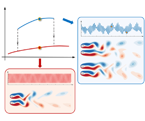
Two examples of the cylinder-scale and cluster-scale IP flows at  $(g^*, Re) = (2.0, 85)$ and (1.0, 55), respectively, are illustrated in figure 5(a,b) for reference. The two IP flows are located in two regions separated by a parameter space occupied by FF flows with IC-0. Both IP flows are characterised by the IP synchronisations of the lifts on the two cylinders. The vortex shedding for the IP flow at
  $(g^*, Re) = (2.0, 85)$ is dominated by merged vortices of identical sign that are shed from individual cylinders, as illustrated in figure 5(a). The vortex shedding pattern for the flow in figure 5(b), however, is mainly featured by the shedding of large-scale vortices from the two cluster shear layers farther downstream from the cylinders. Vortex shedding around individual cylinders for the IP flow in figure 5(b) is very weak and the periodic lateral swing of gap flow is mainly induced by vortices shed from the cluster shear layers. The present observations of IP flows with cluster-scale features also agree with the findings by Carini et al. (Reference Carini, Giannetti and Auteri2014b), where the small gap eddies in the IP base flow at
  $g^* = 0.7$ are transported between two subsequent big vortices and shed from the outer shear layer on the opposite cylinder side.

Figure 5. Typical lift force coefficient,  $C_L$, and flow features for (a) the IP flow with cylinder-scale characteristics; (b) the IP flow with cluster-scale characteristics; (c) the AP
 $_B$ flow; and (d) the IP
 $_B$ flow.
The other flow states newly identified in figure 4 is the synchronised biased IP (IP $_B$) and biased AP flow (AP
 $_B$) strips denoted by the regions with inclined blue and purple lines, respectively. The force and flow characteristics of the AP
 $_B$ regime presented in figure 5(c) show that two Kármán vortex streets formed behind the cylinders are no longer mirror reflections of each other as in AP flow (figure 3c). The gap flow in the AP
 $_B$ flow is inclined towards one direction (towards the top in figure 5c) over the vortex shedding period. This asymmetric feature can also be inferred from the evolution of
  $C_L$ on each cylinder, whereby large and small amplitudes of lift oscillations are observed on Cy1 and Cy2, respectively. Similar flow features have been observed in steady approaching flow past two square cylinders in a side-by-side arrangement (Ma et al. Reference Ma, Kang, Lim, Wu and Tutty2017), but not reported for two circular cylinders, to the best knowledge of the authors. The IP
 $_B$ occurs in a region among FF flows at relatively high
  $Re$ (
 $0.6 < g^* < 0.9$,
  $69 < Re < 90$ in figure 4). Figure 5(d) shows the force and flow features of a typical IP
 $_B$ regime at
  $(g^*,Re) = (0.8, 70)$, where the gap flow is biased downwards. The lift oscillations of both cylinders are periodic with time, mainly due to vortex shedding from Cy1 and cluster-scale vortex shedding in the far wake. Even though the gap shear layers undergo cyclic oscillations over each vortex shedding period (not shown here), they remain biased downwards. The large inclination angle of the gap flow suppresses the vortex shedding from Cy2 and induces a considerable separation distance between shear layers around Cy1.
The FF flow is observed at intermediate  $g^*$ values when the flow transits from a cluster-scale dominated flow feature to a cylinder-scale dominated feature, as shown by the region flooded with grey in figure 4. For the purpose of comparison, the marginal curves for FF1 and FF2 modes identified by Carini et al. (Reference Carini, Giannetti and Auteri2014b, Reference Carini, Auteri and Giannetti2015) are plotted as dotted blue and purple lines, respectively. As will be discussed in the following paragraphs, the flow in the region indicated by filled circles in purple can be either IP or FF depending on the disturbance in the flow. Therefore, the FF flow obtained from IC-0 in this region is denoted as FF
 $_C$ (‘
 $_C$’ for conditional) herein. The regions flooded by blue either side of the FF
 $_C$ region are occupied by conditional FF flows, which will be elaborated further in the subsequent discussion.
The present study focuses primarily on the bifurcations associated with the IP/FF $_C$ and IP/AP flow states. The following three highlights are noteworthy by comparing the present DNS results and Floquet analysis results from Carini et al. (Reference Carini, Giannetti and Auteri2014a,Reference Carini, Giannetti and Auterib, Reference Carini, Auteri and Giannetti2015):
(i) the lower branch of FF1 marginal curves by stability analysis is identical to the lower-bound boundary of FF flows predicted by DNS;
(ii) a new branch of FF flows with solid purple circles, i.e. FF
$_C$, is discovered by DNS with IC-0 but not by the Floquet analysis based on the IP base flow;(iii) a noticeable difference between the results of DNS and Floquet analysis near the lower branch of the FF2 marginal curve is observed.

The following analyses and discussions are centred around interpretation of the features observed above. It will be demonstrated that the presence of the flow state in the parameter range occupied by the FF $_C$ state and the orange shaded area is dependent on IC.
Similarities between flows around two circular cylinders and two square cylinders reported by Mizushima & Hatsuda (Reference Mizushima and Hatsuda2014) are observed. The parameter subspaces of IP–FF1, AP, FF2 and FF $_C$ defined in this study correspond respectively to the II, III, IV-2 and IV-1 regions (figure 3b) by Mizushima & Hatsuda (Reference Mizushima and Hatsuda2014). The feature (i) observed above is likely because the origin of the FF1 flow is synchronised IP Kármán wakes, as pointed out by Carini et al. (Reference Carini, Giannetti and Auteri2014b). The solution of transition from the steady base flow to the IP state in this region is unique based on the findings from two square cylinders, meaning that the use of the IP base flow in stability analysis is appropriate, and the transition to the FF flow in this region is non-bistable accordingly. The interpretations of feature (ii) need more elaboration. Judging based on the findings by Mizushima & Hatsuda (Reference Mizushima and Hatsuda2014), a probable cause for the feature (ii) is that the bistable state of the IP or the AP single mode (region IV-1 in figure 3b) exists over the parameter subspace of FF
 $_C$ and it is stable or unstable to FF instabilities, respectively. The cause of feature (iii) is the emergence of synchronised AP
 $_B$ flow prior to the onset of FF flows, which is somewhat identified as the secondary instability to the IP base flows. This aspect will be elaborated further in the subsequent discussion.
3.1. Phase evolution
The dominant peak of  $\varPsi _k$, i.e.
  $\varPsi _{k-p}$, and the standard deviation of
  $\varPsi _k$ over
  ${T_a}$,
  $\sigma$, are examined along the lines of
  $g^* = 1.5$ and
  $Re = 60$ based on DNS with IC-0 in figure 6 with
  $T_a = 1000$ to investigate potential bifurcation routes of the flow. The filled symbols and error bars represent the values of
  $\varPsi _{k-p}$ and
  $\sigma$, respectively. Different flow states are indicated by different symbols. The following features are noteworthy.

Figure 6. Variations of the maximum probability phase of  $\varPsi (t)$, i.e.
  $\varPsi _{k-p}$, at (a)
  $(g^*, Re) = (1.5, 55\text {--}78)$ and (b)
  $(0.7\text {--}3.5, 60)$ with IC-0. The statistical period is
  $T_a = 1000$. The black vertical bars indicate the standard deviation
  $\sigma$ of
  $\varPsi _{k-p}$ over
  $T_a$.
(I) At  $g^* = 1.5$, as shown in figure 6(a), the synchronised IP flow at
  $Re < 56.5$ is featured by
  $\varPsi _{k-p} = 0$ and
  $\sigma = 0$ as expected. As
  $Re$ is furthered increased beyond the IP flow range,
  $\varPsi _{k-p}$ suddenly shifts to
  ${\sim }{\rm \pi}$ with a non-zero
  $\sigma$ in the FF
 $_C$ state and reverts back to zero in the IP state at
  $Re > 71.5$. This observation indicates that the FF
 $_C$ is possibly bifurcated from the AP synchronisation state.
(II) The synchronisation feature of the flow undergoes changes in a sequence of IP–AP–IP–AP with increasing of  $g^*$ values at
  $Re = 60$ (figure 6b). The value of
  $\varPsi _{k-p}$ varies gradually from 0 to
  ${\rm \pi}$ with a non-zero
  $\sigma$ as
  $g^*$ increases in the FF1 region (the area flooded by green). At the onset of FF
 $_C$,
$_C$,  $\varPsi _{k-p}$ stables at
  ${\sim }{\rm \pi}$ at
  $g^* = 1.35 \text {--} 1.85$ and is located between
  ${\rm \pi} /2$ and
  ${\rm \pi}$ as
  $g^*$ further increases. This again suggests the two wakes in the FF
 $_C$ flow are largely in the AP synchronisation. The value of
  $\varPsi _{k-p}$ suddenly shifts to 0 in the periodic IP state and returns back to
  ${\rm \pi}$ in the periodic AP state at
  $g^* = 2.25$ and 3.0, respectively.
(III) The nearly zero values of  $\sigma$ in the IP and AP states indicate the gap flow constitutes periodic oscillation and non-oscillation over the vortex shedding period,
  $T$, respectively. The non-zero
  $\sigma$ value displayed by the FF flow suggests the gap flow undergoes FF over the period other than
  $T$. The larger the
  $\sigma$, the more unstable the gap flow is.
3.2. Stabilities of IP and AP base flows
The Floquet analysis introduced in § 2.2 is then conducted to investigate the cause for the feature (ii) and is discussed in the following paragraphs.
To start with, the linear stability analysis based on the IP base flow is conducted along seven vertical lines for  $g^* = 0.8 \text {--} 1.8$, as shown in figure 7(a), where the grey and blue shadows represent cases with stable and unstable Floquet multiplier(s), respectively. The critical bifurcation points for the onset of instability are estimated by using a linear interpolation of
  $|\mu |$ to unity. The neutral stability curve for the onset of FF instability obtained from Floquet analysis on the IP base flow is plotted as the dashed orange line in figure 7(a). To facilitate further discussion, the marginal curves obtained from Carini et al. (Reference Carini, Giannetti and Auteri2014a,Reference Carini, Giannetti and Auterib, Reference Carini, Auteri and Giannetti2015) and the boundaries estimated from the present DNS with IC-0 are plotted in figure 7(a). More precisely, the solid green and purple lines represent respectively the marginal curves of IP and AP modes tracked out through the global stability analysis based on the steady symmetric base flow by Carini et al. (Reference Carini, Giannetti and Auteri2014a), the FF1 and FF2 marginal curves reported by Carini et al. (Reference Carini, Giannetti and Auteri2014b, Reference Carini, Auteri and Giannetti2015) are shown by the dotted blue and purple lines, and the boundary between FF and IP flows identified from DNS with IC-0 is indicated by the dashed green line.

Figure 7. Bifurcation diagrams of Floquet analyses based on (a) the IP periodic base flow along  $g^* = 0.8 \text {--} 1.8$, and (b) the AP periodic base flow along
  $g^* = 1.5 \text {--} 2.0$. The shaded areas are the cases where Floquet analyses were conducted. The grey and blue areas represent the cases with stable and unstable Floquet multiplier(s), respectively. The symbols with different colours in (a) are the flow state distributions obtained from the DNS by initialising the flow from an IP flow with IC-
 $Re_L$ or IC-
 $Re_H$. Neutral stability curves associated with the IP and AP periodic base flows in (a) and (b) are plotted as dashed orange and magenta lines, respectively.
For the cases with  $g^* < 1.4$, the lower-bound
  $Re$ values for the onset of instability to IP base flow in figure 7(a) are consistent with the FF1 marginal curve predicted by Carini et al. (Reference Carini, Giannetti and Auteri2014b) and the present DNS with IC-0. In the vicinity of
  $g^* \sim 1.5$, the FF
 $_C$ flow predicted by DNS is not captured by the linear stability analysis based on IP base flow, identical to the results reported by Carini et al. (Reference Carini, Auteri and Giannetti2015). For the cases with
  $g^*> 1.5$ in the FF2 region, both the lower- and upper-bound
  $Re$ values with unstable Floquet multipliers are close to those identified by Carini et al. (Reference Carini, Auteri and Giannetti2015), but are noticeably different from those results predicted by DNS with IC-0 as:
(I) Firstly, the lower-bound
$Re$ for FF flows predicted by the present Floquet analysis on the IP base flow is $Re \sim 51.39$ at $g^* = 1.8$ (the blue shadow in figure 7a), which is noticeably different from those predicted by DNS with IC-0 ($Re \sim 54.5$). This is because the AP and AP$_B$ flows emerge in a narrow strip of parameter space (e.g. $Re = 51.5 \text {--} 54.5$ at $g^* = 1.8$) prior to the onset of FF flows. Those flows are deemed unstable by Floquet analysis is because the vortex shedding frequency of the IP base flow used in the analysis differs substantially from that of the actual AP flow in the region, leading to a pair of unstable complex multipliers in the stability analysis.(II) Secondly, the upper-bound critical
$Re = {\sim } 58.53$ for the FF flows predicted by Floquet analysis on the IP base flow is lower than the critical $Re = {\sim } 64.5$ from DNS with IC-0. The cause of this contradiction is because the FF flow at $g^* = 1.8$ for $Re = {\sim }58.5 \text {--} 64.5$ is located in the FF$_C$ region and cannot be captured by the Floquet analysis on the IP base flow.


Next, a linear stability analysis based on the AP periodic base flow is conducted at  $g^* = 1.5$, 1.8 and 2.0 as revealed in figure 7(b). The regions with stable and unstable Floquet mode(s) and the boundary lines are labelled in the same manner as those in figure 7(a). The neutral stability curve obtained from the Floquet analysis on the AP base flow is plotted as the dashed magenta line in figure 7(b).
For the cases at  $g^* = 1.5$, the predicted lower-bound
  $Re = {\sim } 55.61$ of the FF
 $_C$ flow largely agrees with the
  $Re$ value predicted by DNS with IC-0 (
 $Re = {\sim } 55.5$), confirming our speculation that the AP base flow is unstable to FF flow instabilities. For the cases of
  $g^* = 1.8$ and 2.0, the predicted lower-bound and upper-bound
  $Re$ values agree neither with DNS nor with the stability results based on IP base flow. The Floquet analysis with the AP base flow is only capable of capturing the critical
  $Re$ values for the onset of AP
 $_B$ flow, with a dominant real multiplier
  $|\mu |>1$. For instance, the predicted lower-bound
  $Re$ values for the onset of AP
 $_B$ flow at
  $g^* = 1.8$ are
  ${\sim }52.02$ and
  ${\sim }52.5$ for the Floquet analysis and DNS with IC-0, respectively.
The stability analysis based on the AP base flow is unable to predict the upper-bound  $Re$ values of the FF
 $_C$ flows, likely caused by the following two reasons. Firstly, the method for generating the AP base flow is not applicable for the flow far away from the AP marginal curve (the purple solid line in figure 7). The vortex shedding frequency predicted by enforcing the symmetry condition at
  $y/D = 0$ can differ substantially from the actual vortex shedding frequency in the vicinity of upper branch of the marginal curves, resulting in unstable complex multipliers in the stability analysis in figure 7(b). In addition, the vortex shedding frequency of the periodic AP flow would differ significantly from that of the periodic IP flow at the same (
 $g^*$,
  $Re$) value. For instance, the Strouhal numbers,
  $St = 0.172$ and
  $St = 0.167$ are predicted for the AP flow and the IP flow at
  $(g^*, Re) = (2.5, 90)$, respectively. Because the AP flow cannot sustain in the IP region, the Floquet analysis based on the AP base flow would resolve the unstable Floquet multipliers.
3.3. The influence of IC
3.3.1. The IP/FF$_C$ bistability

The bistability nature of the base flow over the parameter space occupied by the FF $_C$ flow is further confirmed through DNS by initialising the flow from an IP state at adjacent lower or higher
  $Re$ values but constant
  $g^*$ for
  $g^*$ from 0.8 to 1.8. The interval of
  $Re$ is fixed as
  $\Delta Re = 1$. To simplify the discussion, the flows initialised from the fully developed instantaneous flow field at adjacent lower or higher
  $Re$ values are denoted as IC-
 $Re_L$ and IC-
 $Re_H$, respectively. Flow states identified with IC-
 $Re_L$ and IC-
 $Re_H$ are marked as discrete symbols in figure 7(a), as labelled in the figure legend. The green arrows represent the directions of successive initialisation. As shown in figure 7(a), the estimated lower- and upper-bound
  $Re$ values for the FF flow agree well with the marginal curves by Floquet analysis on the IP base flow. This is attributed to the fact that the perturbation level introduced to the IP flow in DNS with successive initialisation is comparable to the infinitesimal perturbations introduced in the Floquet analysis of the IP base flow. The flow remains in the IP state without transitioning to FF flow over the parameter range where FF
 $_C$ flow is predicted with IC-0. This outcome also suggests that the transitions from IP to FF
 $_C$ in both directions are bistable, depending on the IC. The FF
 $_C$ state would develop when the flow is initiated from the AP synchronisation state or sufficiently large perturbations are introduced into the IP flow. During the simulation, the AP flow becomes unstable to the FF instability, leading to the FF
 $_C$ state identified in the stability analysis with AP base flows and DNS with IC-0.
We further infer that the transition from the FF $_C$ state to the IP state is irreversible. To confirm this inference, DNS is conducted again at
  $g^* = 1.5$ by initialising the flow from a fully developed FF
 $_C$ state with IC-
 $Re_L$ and IC-
 $Re_H$. The resulting flow states are detailed in figure 8(a). The IP and FF
 $_C$ flow states are represented by the bottom and top horizontal lines, respectively. The thick grey line indicates the presence of flow states based on DNS with IC-0. The starting point and direction for successive initialisation are marked by the solid star symbol and solid line with an arrow, respectively. Surprisingly, the upper- and lower-bound
  $Re$ values for the transition from the FF
 $_C$ state to the IP state at
  $g^* = 1.5$ with IC-
 $Re_L$ and IC-
 $Re_H$ are higher and lower respectively than their counterparts obtained by DNS with IC-0, as shown by the two extended regions shaded by blue in figure 8(a). This result indicates that not only the emergence of the FF
 $_C$ flow but also the parameter range over which the FF
 $_C$ flow develops is dependent on the IC. The extended parameter spaces of the presence of the FF
 $_C$ state at
  $g^* = 1.3 \text {--} 1.6$ with IC-
 $Re_L$ and IC-
 $Re_H$ are labelled by two strips in blue in figure 4.

Figure 8. Comparisons of the flow state distributions obtained by different IC at (a)  $g^* = 1.5$, (b)
  $g^*= 0.8$, (c)
  $g^* = 1.8$ and (d)
  $Re = 60$. The IP, AP/AP
 $_B$ and FF flow states are represented by horizontal lines. The thick grey lines represent the presence of flow states based on DNS with IC-0. The solid lines with arrows in different colours represent the dominance of flow states based on the simulations initialised by a fully developed flow field from the adjacent lower/higher
  $Re$ or
  $g^*$ value (
 $\Delta Re = 1$,
  $\Delta g^* = 0.1$), where the starting points are marked as solid stars. The areas shaded by grey and blue represent the bistable IP/FF
 $_C$ regions.
The same transition checks are conducted at  $g^* = 0.8$ and 1.8. The resulting flow states in different transition routes are shown in figure 8(b,c), in a similar manner as those in figure 8(a). As expected, no hysteresis is detected near the lower-bound
  $Re$ values of the FF1 state at
  $g^* = 0.8$ (figure 8b). The outcome suggests that the lower bound of the FF1 instability region is associated with the supercritical Neimark–Sacker bifurcation. Similarly, for the transition checks at
  $g^* = 1.8$ in figure 8(c), no bistability is discovered near the lower
  $Re$ bound of the FF2 state. The transitions from AP
 $_B$ to FF2 states in both directions are insensitive to the initial conditions and bifurcate at
  $Re \sim 54.5$ for
  $g^* = 1.8$. Nevertheless, the existence of the IP/FF
 $_C$ bistability is observed at
  $Re = 58.5 \text {--} 64.5$ for
  $g^* = 1.8$, as shown by the grey shaded range in figure 8(c). While the flow remains FF
 $_C$ until
  $Re = 64.5$ by initiating the flow from an FF
 $_C$ flow starting from
  $Re = 59$, the flow stays in an IP state until
  $Re = 58.5$ by initiating the IP flow starting from
  $Re = 65$. This bistable
  $Re$ range also agrees with the result reported in § 3.2 that the predicted upper-bound
  $Re$ values for the FF flow through the Floquet analysis on the IP base flow are much lower than those estimated from the DNS with IC-0. This bistability bifurcation agrees with the conjecture proposed by Carini et al. (Reference Carini, Auteri and Giannetti2015) that the instability region above the upper branch of FF2 at
  $g^* = 1.8$ is sensitive to IC, suggesting a subcritical nature of the Neimark–Sacker bifurcation.
We now consider the bistable feature at a fixed  $Re$ by continuously increasing or decreasing
  $g^*$, i.e. IC-
 $g^*_L$ and IC-
 $g^*_H$, respectively. A set of simulations is carried out at
  $Re = 60$ over the range of
  $g^*$ values from 1.1 to 2.5. The flow passes through the FF1 instability region, the bistable IP/FF
 $_C$ region and the IP region on increasing
  $g^*$. The interval for
  $g^*$ is selected as
  $\Delta g^* = 0.1$. In these new simulations, the computational meshes at different
  $g^*$ values were designed to have identical mesh typology and number of nodal points. This set-up enabled a simple mapping of the fully developed flow field at the adjacent upper or lower
  $g^*$ value onto the mesh at the desired
  $g^*$ value. That is, for instance, the initial condition of the flow at
  $(g^*, Re) = (1.5, 60)$ with IC-
 $g^*_H$ is obtained by mapping a fully developed instantaneous flow field at
  $(g^*, Re) = (1.6, 60)$ to the mesh with
  $g^* = 1.5$. Each simulation is carried out for 3000 non-dimensional time units to obtain fully developed flow on the new mesh. Five bifurcation routes starting from an IP state or an FF
 $_C$ state are considered, as illustrated in figure 8(d). Although the meshes used for different
  $g^*$ with non-zero initial conditions are slightly different from those with IC-0, similar results are observed in the bistable IP/FF
 $_C$ region, whereby an FF
 $_C$ state is reached as well at
  $g^* = 1.35 \text {--} 2.15$ by initialising from an FF flow, while the flow stays in IP by starting the flow from an IP state. The flow states are unique in both FF1 (
 $g^* < 1.35$) and IP (
 $g^* > 2.15$) regions.
3.3.2. The IP/AP bistability
Similar bistability checks are also conducted between cylinder-scale IP and AP flow states observed at  $g^* = 2.0 \text {--} 3.5$. The simulations with IC-
 $Re_L$ at
  $g^* \leq 2.75$ are initiated from a fully developed IP flow at an adjacent lower
  $Re$, while the IP initial condition for
  $g^* \ge 2.75$ is obtained using the same mapping strategy as in figure 8(d) by continuously mapping the IP flow at
  $(g^*, Re) = (2.75, 60)$ to the targeted mesh at large
  $g^*$ values. Considering the large parameter space covered in this region, the interval of
  $Re$ is no longer a fixed value. A general interval of
  $\Delta Re = 5$ is selected but a fine resolution of
  $\Delta Re = 1$ is chosen on approaching the boundaries.
The bifurcation features are somewhat similar to the bistable IP/FF $_C$ region, as shown by the strip coloured in orange in figure 4. In this region, the flow stays in the IP state by successively initialising the flow from an IP flow with IC-
 $Re_L$ outside the bistable parameter region. Because the coupling between two wakes decreases as
  $Re$ is increased, the IP flow with IC-
 $Re_L$ cannot be sustained while
  $Re$ is further away from the dashed red line in figure 4 (the onset of the AP flow predicted by DNS with IC-0). In the present case, the lower-bound
  $Re$ values for the AP flows, when the flow is initiated with IC-
 $Re_H$ within the AP flow parameter range (i.e. initiated by an AP flow with a higher
  $Re$), remain identical to those obtained by DNS with IC-0. One of the reasons for this behaviour might be that the perturbation level contained in the AP background flow is not sufficient to cause a change of flow from AP to IP in the parameter range. The outcomes mentioned above suggest that the bistable IP/AP state is reversible. Note that the boundaries in the bistable IP/AP region may be slightly affected by the
  $Re$ increment employed in the simulation, although no further check is conducted to explore this aspect.
4. Discussion
In § 3, we provided a detailed discussion on the bistability phenomenon with the merits of the phase dynamics, Floquet analysis based on both IP and AP periodic base flows and DNS with different IC. Two bistable regions, i.e. bistable IP/FF $_C$ and bistable IP/AP, are identified at small and large
  $g^*$ values, respectively. According to the regime distributions in figure 4, the dominant flow features at intermediate
  $g^*$ values gradually transits from cluster-scale to cylinder-scale vortex shedding processes with increasing
  $g^*$, leading to complex flow features, such as the FF, IP
 $_B$, AP
 $_B$ states, in the narrow strip of the parameter space bounded by the IP mode boundary (the green solid line in figure 4) and the boundary between FF flow and the IP regime with IC-0 (the dashed green line in figure 4). The IP flows on the bottom left and top right of the bistable IP/FF
 $_C$ region correspond respectively the cluster-scale and cylinder-scale vortex shedding processes behind two cylinders, as evidenced by the flow features in figure 5(a,b). In addition, the cylinder-scale IP and AP states form at strong and weak couplings, respectively, judging based on the sequence of their emergence in terms of increasing
  $g^*$.
Given the above findings, it is reasonable to conclude that the cluster-scale AP state would develop at intermediate  $g^*$ values. However, the periodic cluster-scale AP flow is not identified in the present regime map. Judging based on the value of
  $\varPsi _{k-p} \sim {\rm \pi}$ at the onset of the FF
 $_C$ state (figure 6a), it is reasonable to believe that the FF
 $_C$ flow is bifurcated from the AP flow with the cluster-scale feature and the bistability IP/FF
 $_C$ occurs over the parameter range where the cluster-scale AP flow state would exist. The bistable IP/FF
 $_C$ region is somewhat similar to the region IV-I reported by Mizushima & Hatsuda (Reference Mizushima and Hatsuda2014), where either the IP or AP mode of instability can survive by itself. As the requirement of the simultaneous shedding of large-scale vortices from the cluster shear layers is overly strict, the cluster-scale AP flow itself is unstable and evolves into the FF
 $_C$ flow.
In the present scenario, the bistable IP/AP region at large  $g^*$ is the normal 1-loop hysteresis phenomenon (type A in figure 1). In contrast, the irreversible bistability between IP and FF
 $_C$ states identified in the present scenario is referred to the ‘isola’ bistability (type C in figure 1). The flow can bifurcate from the isola branch (FF
 $_C$) to the continuous branch (IP) with varying
  $Re$, but the IP flow itself cannot revert back to the isola by simply varying the
  $Re$ in the opposite direction. Once the flow develops into one state, e.g. the FF
 $_C$ state, the characteristics of the flow state are independent of how the flow is resolved, e.g. continuously increasing or decreasing
  $Re$. This conjecture can be confirmed first through the dominance of the FF
 $_C$ in the blue strips in figure 8(a) by initiating the flow from a fully developed FF
 $_C$ flow with IC-
 $Re_L$ and IC-
 $Re_H$. No hysteresis is detected for the upper and lower bounds of
  $Re$. That is, for instance at
  $g^* = 1.5$, the lower bound of the
  $Re$ value remains
  $Re = 54.5$ no matter the flow is initiated from an FF
 $_C$ flow at
  $Re = 57$ or
  $Re = 55$ with IC-
 $Re_H$. Moreover, the phase characteristics of the FF flow with zero and non-zero initial conditions are checked at
  $g^* = 1.5,\ 1.8$ and
  $Re = 60$, as depicted in figure 9. The features of the FF flow are statistically quantified using the values of
  $\varPsi _{k-p}$ and
  $\sigma$ over the statistical period of
  $T_a = 1000$. As shown by the figure legend in each plot, the
  $\varPsi _{k-p}$ and
  $\sigma$ values for cases with different IC are represented by continuous lines and black error bars or shaded areas with colours, respectively. The starting point for the successive initialisation is marked by the solid star symbol. The values of
  $\varPsi _{k-p}$ and
  $\sigma$ for the FF flows with non-zero IC are largely identical to those obtained from IC-0, suggesting that the characteristics of the FF
 $_C$ flow are insensitive to the way
  $Re$ is varied.

Figure 9. Variations of the maximum probability phase of  $\varPsi (t)$, i.e.
  $\varPsi _{k-p}$, at (a)
  $(g^*, Re) = (1.5, 55 \text {--} 78)$, (b)
  $(g^*, Re) = (1.8, 51 \text {--}65)$ and (c)
  $(0.7 \text {--} 2.75, 60)$ with different IC. The statistical period is
  $T_a = 1000$. The black vertical bars and shaded areas indicate the standard deviation
  $\sigma$ of
  $\varPsi _{k-p}$ with zero and non-zero IC.
The outcomes mentioned above support the conjecture that the bistable IP/FF $_C$ states are only determined by the perturbation levels in the initial stage of the simulation. Once the IP flow is utilised as the initial condition, the level of perturbations in the flow initiated by successive initialisation from an IP state is not enough to force a transition from the IP state to the FF
 $_C$ state. The flow remains as IP regardless of continuously increasing or decreasing
  $Re$. In contrast, the FF
 $_C$ flows are highly unstable, as suggested by the large value of
  $\sigma$ for FF
 $_C$ flows observed in figure 9. When the flow is initiated from an FF
 $_C$ state, the perturbation level in the flow is likely higher than those initiated with the IC-0 or IP state, leading to the presence of the FF flow in the blue strips in figure 4. This FF flow has to transit to the IP state when the IP coupling becomes strong enough.
Apart from the irreversible bistability mentioned in § 3, another type of bistability, where two equilibrium states of IP and AP occur intermittently over the temporal space, are observed in the vicinity of the AP marginal curve. An example of the temporal variations of lifts on the cylinders, phase dynamics and snapshots of vorticity contours at  $(g^*, Re) = (1.6, 54)$ with IC-0 is presented in figure 10. The temporal variation of total
  $C_L$ on the cluster shows a feature that the FF flow is dominated by the IP and AP synchronisations occurring alternatively in the temporal space, judging based on the respective large and small magnitudes of
  $C_{Total}$. This feature is also confirmed by
  $\varPsi (t)$ shown in figure 10(b). The phase rotates in the IP torus for an epoch shaded in green before it shifts to the AP torus for another epoch. Instantaneous flow fields selected from a time instant in each synchronisation state are shown in figure 10(c,d). The IP and AP dominated synchronisation states are evident at
  $t^* = 6000$ and 6300, respectively. A further examination of the flow features (not shown here) reveals that the flow is also characterised by a flapping gap flow in each of IP and AP dominated stages. It is noteworthy that the present bistability, where synchronised IP and AP dominated FF flows result in beating-like waveforms, is different from the bistable states reported in § 3 where either IP or FF
 $_C$ appear, depending on the IC. The present observation also agrees with the speculation proposed by Carini et al. (Reference Carini, Auteri and Giannetti2015) that the quasi-periodic features of the FF flow at large
  $g^*$ might be associated with the nonlinear interaction between the IP and AP states.

Figure 10. Force, phase and flow characteristics of the flow at  $(g^*, Re) = (1.6, 54)$ with IC-0. (a) Time traces of the lift coefficients on Cy1, Cy2 and Total. (b) The evolution of phase dynamics of
  $\varPsi (t)$. Flow fields at corresponding (c) IP and (d) AP synchronisation states.
We believed that the bistabilities discovered at relatively low  $Re$ values could potentially persist at high
  $Re$ values. We found that the FF flow becomes desynchronised and chaotic as
  $Re$ is increased beyond a critical
  $Re$ in the top-left corner of the FF parameter space. Figure 11 displays an example of the desynchronised FF flow at
  $(g^*, Re) = (0.9, 200)$. The desynchronised features of the FF flow can be clearly detected from the lift coefficient time histories in figure 11(a), where both lifts on Cy1 and Cy2 experience random oscillations with time. A dominant feature of the phase evolution in figure 11(b) is that
  $\varPsi (t)$ drifts randomly with time, suggesting the wakes behind the two cylinders are desynchronised with each other. To investigate the synchronisations between the two wakes, the histogram distributions of
  $\varPsi (t)$ for stage (i) to stage (iii) are shown in figure 11(c), where intermittent switching between IP and AP states over the temporal space is identified.

Figure 11. (a) Force and (b) phase evolution for the FF flow at  $(g^*, Re) = (0.9, 200)$. (c) Histograms of
  $\varPsi (t)$ over the statistical periods shaded in (a,b).

Figure 12. Similar to figure 8 but for transitions of regimes A–F–D–A in the scenario of oscillatory flow past four cylinders in a diamond arrangement (Ren et al. Reference Ren, Cheng, Tong, Xiong and Chen2019) at gap ratio,  $g^* = 0.5$, and Keulegan–Carpenter number,
  $\textit {KC} = 7$.
We therefore believe the intermittent jumping between IP and AP dominated states observed here is directly caused by the instability associated with cluster-scale IP base flow. The highly unstable flip-flopping feature forces the transition from the cluster-scale IP flow state to the other AP flow state. It is also shown that the desynchronised FF flow is dominated by the IP state at relatively low  $Re$, e.g.
  $Re= 90$, while the AP state dominates at high
  $Re$. Since the boundary layer thickness on the cylinder surface is inversely proportional to the
  $\sqrt {Re}$, the increase of
  $Re$ has similar effect on the flow to increasing the
  $g^*$ value, which is behind the above observations. We also believe the understanding of the bistability phenomenon in the present scenario is crucial for interpreting the intermittently quasi-periodic dynamics in other bluff-body flows.
Based on the understanding gained through the present study, we believe the bistability transition features are not limited to the present scenario. To substantiate this claim, we checked the oscillatory flow past four cylinders in a diamond arrangement reported by Ren et al. (Reference Ren, Cheng, Tong, Xiong and Chen2019). In their study, an abnormal phenomenon, where regime F and regime D flows were found in a parameter surrounded by regime A flow at  $g^* = 0.5$ and Keulegan–Carpenter number
  $\textit{KC} = 7$, was discovered (figure 4a in Ren et al. Reference Ren, Cheng, Tong, Xiong and Chen2019). Following a revisit of the problem with DNS, irreversible bistability is found where the abnormal phenomenon occurs, as shown in figure 12. While the transition sequence of regimes A–F–D–A is observed with IC-0, the sequences of regimes A–F and regimes F–A are discovered by initiating the flow with IC-
 $Re_L$ and IC-
 $Re_H$ respectively. When the DNS is initiated with IC-
 $Re_L$ and IC-
 $Re_H$ in regime D, flow remains in regime D and jumps back to regime F then regime A respectively. Once the regime D flow jumps back to regime A, it is unable to revert back to regime D again, demonstrating the irreversible transition nature of the flow. This example confirms the existence of irreversible bistability in flows other than the present problem, although the transitions are not exactly the same.
Finally, it is noteworthy that the present Floquet analysis and DNS results are slightly different from the results reported by Carini et al. (Reference Carini, Giannetti and Auteri2014a, Reference Carini, Auteri and Giannetti2015) in the following aspects,
(i) The left branch (with respective to the IP–AP codimension-two bifurcation point) of the neutral stability curve obtained from Floquet analysis on the AP base flow (the dashed magenta line in figure 7b) falls slightly below the AP mode curve by Carini et al. (Reference Carini, Giannetti and Auteri2014a).
(ii) The upper-bound value of
$Re$ (${\sim } 58.53$) for $g^* = 1.8$ determined based on the present Floquet analysis on the IP periodic base flow, is slightly lower than that given by Carini et al. (Reference Carini, Auteri and Giannetti2015) ($Re \sim 59.84$).


Those two differences are possibly due to the differences in the numerical approaches and domain sizes employed in the present study and in Carini et al. (Reference Carini, Giannetti and Auteri2014a). We know that the AP mode in Carini et al. (Reference Carini, Giannetti and Auteri2014a) has features such as,
(I) individual vortex shedding is generated around each cylinder;
(II) the flow satisfies the reflection symmetry condition (2.5);
(III) the vertical velocity
$v = 0$ and $\omega _z = 0$ at $y/D = 0$;(IV) the mixing mechanism of shear layers in the vicinity of
$y/D = 0$ is somewhat negligible in the vicinity of the AP marginal curve.


These characteristics are somewhat similar to the condition of the flow around two cylinders with a symmetry wall ( $\partial u/\partial y = 0$ and
  $v = 0$) at
  $y/D = 0$. Although the symmetry wall is not actually present in the case of the AP mode, the line with
  $\omega _z = 0$ between two gap shear layers in the AP mode is considered as equivalent to a symmetry wall, with a much weaker confinement effect. Therefore, we believe the critical
  $Re_{SW\text {-}cr}$ for onset of vortex shedding of the symmetry wall case can largely represent the AP marginal curve. With this in mind, instead of performing same global stability analysis on the steady base flow as that in Carini et al. (Reference Carini, Giannetti and Auteri2014a), a set of DNS tests is conducted by imposing the symmetry condition at
  $y/D = 0$ for
  $g^* = 1.3 \text {--} 2$; and the cases are simulated on the top half domain only. The variation of
  $Re_{SW\text {-}cr}$ with respect to
  $g^*$ is plotted as the dashed grey line in figures 4 and 7. The present
  $Re_{SW\text {-}cr}$ curve is slightly lower than the AP marginal curve by Carini et al. (Reference Carini, Giannetti and Auteri2014a) for
  $g^* < 2.0$ and collapses with the AP marginal curve at
  $g^* > 2.0$. The small difference between
  $Re_{SW\text {-}cr}$ and the AP marginal curve (
 $\Delta Re \leq 1$) is possibly due to the numerical schemes and computational domain sizes. Both the onset of FF
 $_C$ and the lower-bound
  $Re$ of Floquet analysis based on the AP periodic base flow agree better with the
  $Re_{SW\text {-}cr}$ curve than the AP mode neutral curve.
In addition, the exact agreement between the upper-bound  $Re$ at
  $g^* = 1.8$ obtained from the Floquet analysis based on the IP base flow and that estimated from the DNS by initialising the flow from an IP state with IC-
 $Re_H$ (the solid orange line in figure 8c) supports the above-mentioned conjecture.
5. Conclusions
The bistabilities of two equilibrium states in coupled side-by-side Kármán wakes are investigated through DNS with different IC and stability analyses on different base flows over a range of gap-to-diameter ratio ( $g^*= 0.2 \text {--}3.5$) and Reynolds number (
 $Re = 47 \text {--} 100$). The significant findings from the present study are summarised below.
(i) The characteristics of flow features at intermediate
$g^*$ values are strongly affected by the dominant characteristic length scales and IP and AP states of synchronised base flows. The flow occurs in the sequence of cluster-scale IP, cluster-scale AP, cylinder-scale IP and cylinder-scale AP with increasing $g^*$ values. The cluster-scale AP flow is inherently unstable to FF instabilities and eventually evolves into the FF flow. Two bistabilities are found in the transitional $g^*-Re$ regions between the IP and AP vortex shedding states.(ii) The flow in the first bistable region (
$g^*= 1.4 \text {--} 2.0$) attains either the IP periodic flow or the FF flow, depending on the IC. The FF flow in the bistable region is denoted as FF$_C$. We demonstrated through both DNS and stability analysis that, in the bistable IP/FF$_C$ region, the flow is stable and unstable to IP and AP base flows, respectively. While the state of flow develops into the FF$_C$ flow when the DNS is initiated from zero IC and from an FF$_C$ state, the IP flow is predicted by initiating from an IP flow in DNS. The flow in the area occupied by FF$_C$ flow can transit to IP flow through continuously varying $Re$ values in either direction with the FF$_C$ flow as initial condition. Once the flow is in the IP branch, it cannot revert back to the FF$_C$ branch regardless of increasing or decreasing $Re$, indicating that the transition from the FF$_C$ branch to the IP branch is irreversible. The parameter range over which the FF$_C$ flow is developed by initiating from an FF$_C$ flow is wider than that through zero IC. This finding suggests that the parameter range of the FF$_C$ flow is sensitive to the IC. The bistability feature of the present flow constitutes the cause of a discrepancy reported in the literature in predicting FF flows by DNS and stability analysis.(iii) The flow state in the bistable IP/FF
$_C$ region is only determined by the perturbation levels in the flow, meaning that once the flow develops into one state, the characteristics of the flow state are independent of the way how the flow is resolved. The perturbation level in the FF$_C$ is likely higher than those initiated with zero IC or IP state, leading to the extension of the FF flow on both ends of the bistable region. On the contrary, while the IP flow is utilised as the initial condition, the level of perturbations in the flow is not enough to force a transition from the IP flow to the FF$_C$ state. The flow remains as IP regardless of continuously increasing or decreasing $Re$.(iv) The second bistability is observed between IP and AP periodic states at large
$g^*= 2.0 \text {--} 3.5$, where the transition is reversible.(v) While linear stability analysis based on the AP base flow is able to predict the lower-bound
$Re$ values of FF$_C$ and AP$_B$ flows, it is incapable of predicting the upper branches of FF$_C$ and FF2 flows. The reasons for this observation are that (a) the symmetry condition imposed at $y/D = 0$ leads to a poor prediction of vortex shedding frequency in the vicinity of the upper branch of the FF flows and (b) the vortex shedding frequency of the periodic AP flow differs significantly from that of the periodic IP flow at the same ($g^*$, $Re$) value, leading to the unstable multipliers in the Floquet analysis.(vi) The bistable phenomena discovered at relatively low
$Re$ values can be useful in interpreting the desynchronised FF flows and other intermittently quasi-periodic flows at high $Re$. The bistabilities and irreversible transitions observed in the present study could also occur in other bluff-body flows.


Acknowledgements
The first author would like to acknowledge the financial support from the China Scholarship Council (CSC). This research was supported by computational resources provided by the National Computational Merit Allocation Scheme (NCMAS) and the Pawsey Supercomputing Centre with funding from the Australian Government and the Government of Western Australia.
Funding
This work was supported by the National Key R&D Program of China (Project ID: 2016YFE0200100) and the Australia Research Council Discovery Grant (Project ID: DP200102804).
Declaration of interests
The authors report no conflict of interest.
Appendix A. Mesh validation
The computational domain, mesh and polynomial order used in this study were chosen based on a thorough parameter dependence check, which was carried out at  $g^* = 1.5$ and
  $Re =100$. The adopted mesh distribution close to the cylinder cluster and the computational domain are shown in figure 2. The distances from the origin of the coordinate system to the inlet, outlet and lateral boundaries are defined as
  $L_i$,
  $L_o$ and
  $L_s$, respectively. The number of discretised macro-elements (
 $N_c$) around the cylinder perimeter equals to 32, which is determined based on other spectral element studies for cylinder wakes, e.g. Henderson & Barkley (Reference Henderson and Barkley1996), Xiong et al. (Reference Xiong, Cheng, Tong and An2018), Elston et al. (Reference Elston, Blackburn and Sheridan2006) and Ren et al. (Reference Ren, Cheng, Tong, Xiong and Chen2019, Reference Ren, Lu, Cheng and Chen2021). The height of the first macro-element next to the cylinder surface is approximately
  $0.03D$. The expansion ratios are kept below 1.4 within the whole computational domain.
The mesh with  $L_i = 50D$,
  $L_s = 50D$ and
  $L_o = 100D$, the polynomial order
  $N_p = 6$ and time step
  $\Delta t = 0.002$ are selected as the reference mesh (called Mesh 1 in table 1) in the dependence check. Three variations of the computational domain size and the mesh resolution are examined by changing the
  $N_p$ and
  $L_o$ in the following manners
(i) For Mesh 2,
$N_p$ is increased from 6 to 8.(ii) For Mesh 3,
$L_o$ is increased to $150D$.(iii) For Mesh 4,
$\Delta t$ is halved to $\Delta t = 0.001$.


Table 1. Influence of the mesh sizes on hydrodynamic force coefficients and Strouhal number (St) of side-by-side cylinder at  $g* = 1.5$ and
  $Re = 100$:
  $N_{el}$ represents the element number;
  $N_p$ is the polynomial order;
  $L_o$ is the length of outflow and
  $\Delta t$ is the time step.

The mesh convergence is checked by comparing the statistical parameters, i.e. Strouhal number ( $St$), the drag coefficient (
 $C_D$) and the lift coefficient (
 $C_L$), which are defined as,
 $$\begin{gather} C_D(t) = F_D(t)/(\tfrac{1}{2}\rho D U^2), \end{gather}$$
 $$\begin{gather}C_L(t) = F_L(t)/(\tfrac{1}{2}\rho D U^2), \end{gather}$$
 $$\begin{gather}St = f_{St}D/U, \end{gather}$$
where  $F_L$ and
  $F_D$ are the time-dependent lift and drag forces on the cylinder per unit length,
  $\rho$ is the fluid density,
  $U$ is the magnitude of the incoming flow velocity. The value of
  $f_{St}$ indicates the dominant frequency of
  $C_L$. The time-averaged lift and drag coefficients are defined as,
  $\overline{C_L}$ and
  $\overline{C_D}$, respectively. The maximum amplitude of lift coefficient fluctuations (
 $C_L'$) is defined as,
 \begin{equation} C_L' = \sqrt{\frac{1}{M}\sum_{i=1}^M (C_{L,i}-\overline{C_L})^2}, \end{equation}
where  $M$ is the sampling size of the statistics. In the present study, the time histories of
  $C_L$ and
  $C_D$ over 1000 non-dimensional time units (
 $t^* = Ut/D$) after the flow becomes fully developed are utilised to acquire data for statistics.

Figure 13. (a) Instantaneous streamwise velocity ( $U$) contour for Mesh 1 at
  $g* = 1.5$ and
  $Re = 100$. (b) Corresponding velocity profiles at
  $x/D = 0.6$ (dotted red line in (a)), sampled at the same phase corresponding to the peaks of the lift coefficient on Cy2 for Mesh 1–4.
As shown in table 1, the results calculated using meshes 2–4 are within 0.2 % of the corresponding values obtained using the reference mesh, suggesting that the reference mesh listed in table 1 is adequate for the numerical simulations of the present study. In addition, the instantaneous streamwise velocity ( $U$) profiles along a vertical line near the cylinder surfaces at
  $x/D = 0.6$ are compared among the meshes listed in table 1. The instantaneous flow field is selected at the phase when the lift coefficient on Cy2 is at its maximum. Figure 13(a) presents a representative contour of the streamwise velocity distribution for the reference mesh (Mesh 1), while the
  $U$ profiles at
  $x/D = 0.6$ among four meshes are compared in figure 13(b). The differences among the four meshes are negligible, with a maximum difference of the streamwise velocity obtained using the above compared meshes (Meshes 2–4) and the reference mesh (Mesh 1) is 0.3 % of the free-stream velocity (
 $u_\infty = 1$).
The mesh convergence is further validated against the simulation results reported in the literature of two side-by-side cylinders at  $g^* = 1.5$ and
  $Re = 100$ (Kang Reference Kang2003; Carini et al. Reference Carini, Giannetti and Auteri2014b, Reference Carini, Auteri and Giannetti2015). It is seen in table 2 that the present force coefficients also compare well with the published results.
Table 2. Comparisons of force coefficients and Strouhal numbers from the reference mesh (Mesh 1) with other numerical results at  $g* = 1.5$ and
  $Re = 100$. The values in the brackets behind hydrodynamic coefficients are the relative errors compared with the present mesh (Mesh 1). IBM: immersed-boundary method.


Figure 14. (a) Time histories of lift coefficients at  $(g^*, Re) = (0.8, 60)$ before and after utilising the BoostConv approach of the steady flow past two side-by-side circular cylinders. The BoostConv is employed in the shaded area. (b) A zoom-in figure for
  $t^* >3000$.

Figure 15. Comparisons of the Floquet multiplier  $|\mu |$ for Floquet analyses on (
 $a$) IP base flows and (
 $b$) AP base flows at
  $(g*, Re) = (1.5, 56\text {--}70)$ with different (
 $K_n$,
  $N_{t,s}$) combinations.
Appendix B. Stabilisation method
In this section, we introduced two stabilisation methods for generating the IP and AP periodic base flows in Floquet analyses:
(i) The stabilisation of periodic unstable cases to IP periodic flows utilises a stabilisation algorithm, namely BoostConv, on a fully developed flow obtained from DNS to minimise the residual norm of fluid quantities, which is identical to that used in Carini et al. (Reference Carini, Giannetti and Auteri2014b, Reference Carini, Auteri and Giannetti2015). A detailed introduction of this method can be found in Citro et al. (Reference Citro, Luchini, Giannetti and Auteri2017). As an example, figure 14 illustrates how the BoostConv approach stabilises an FF flow for
$t^* > 3000$. For each case, the BoostConv approach lasts for at least $1000 t^*$ to obtain a fully developed solution. After that, 32 equi-spaced time slices ($N_{t,s}$) over one vortex shedding period are selected to reconstruct the base flows.(ii) To generate the AP base flows, simulations are conducted by inserting a symmetry wall at
$y/D = 0$ across the domain. The boundary conditions, except for $\partial u/\partial y = 0$ and $v = 0$ for the symmetry wall, are identical to those employed in DNS. The placement of the symmetry wall at $y/D = 0$ effectively removes the interaction of cluster shear layers and artificially force the flow to hold the reflection symmetry. After the fully developed flow is established around each cylinder, the $N_{t,s}=32$ equi-spaced time slices over one vortex shedding period are projected onto the full computational domain without the symmetry boundary in the middle.


Detailed selections of  $N_{t,s}$ for Floquet analysis will be introduced in Appendix C.
Appendix C. Convergence checks for Floquet analyses
Finally, the sensitivity of the Floquet analysis to the choice of the  $N_{t,s}$ snapshots per vortex shedding cycle and the
  $K_n$ dimensions of Krylov subspace is also investigated. Since the major scope of the paper is on the bistable IP/FF
 $_C$ region, the sensitivity checks on both IP and AP base flows are performed at
  $g^* = 1.5$ and
  $Re = 56 - 70$. The results of
  $K_n = 16$ and
  $N_{t,s} = 32$ are selected as the reference. Three combinations by changing
  $K_n$ from 16 to 32 and
  $N_{t,s}$ from 32 to 64 are examined. Corresponding results on the four (
 $K_n$,
  $N_{t,s}$) combinations for the Floquet analyses based on IP and AP base flows are shown in figures 15(
 $a$) and 15(
 $b$), respectively. The dominant Floquet multiplier
  $|\mu |$ obtained from the other three (
 $K_n$,
  $N_{t,s}$) sets are less than 1 % of the corresponding values obtained using the reference
  $(K_n, N_{t,s}) = (16, 32)$, suggesting that further increasing
  $N_{t,s}$ and
  $K_n$ would not affect the
  $|\mu |$ values. Therefore, the present selections of 32 equi-spaced base flows over one vortex shedding period and 16 dimensions of Krylov subspace are adequate for the Floquet analyses.


