1. INTRODUCTION
Descriptions of various solutions to the problem of drafting trajectories for ships based on automatic identification system (AIS) historical data can be found in several publications (Anneken et al., Reference Anneken, Fischer and Beyerer2015; Borkowski, Reference Borkowski2017; Breithaupt et al., Reference Breithaupt, Copping, Tagestad and Whiting2017; George et al., Reference George, Crassidis, Singh and Fosbury2011; Lane et al., Reference Lane, Nevell, Hayward and Beaney2010; Ristic et al., Reference Ristic, La Scala, Morelande and Gordon2008; Sang et al., Reference Sang, Yan, Wall, Wang and Mao2016). The majority of them contain solely the results of the research, the main aims of which were to develop methods of detecting abnormalities and forecasting ship movement.
Based on the theory of conformal prediction, Laxhammar and Falkman (Reference Laxhammar and Falkman2011, Reference Laxhammar and Falkman2014) presented the Similarity-based Nearest Neighbour Conformal Anomaly Detector (SNN-CAD). As the name implies, it is a combination of the Conformal Anomaly Detector (CAD) and Similarity-based Nearest Neighbour (SSN) with implementation of the Hausdorff distance. CAD is a general anomaly detection method that is, in fact, a two-class conformal predictor. In CAD, each example (e.g. trajectory) is compared with the whole set of examples; the dissimilarity of the example to all other examples is then calculated. An example is considered to be an anomaly once its dissimilarity is higher than that of other examples in the set. In SSN-CAD, the Hausdorff distance is used to measure dissimilarity, which can be successfully applied to trajectories of different length. A modified version of this method, SHNN-CAD +, in which the Hausdorff distance measure has been improved and which takes into account the difference in direction, can be found in research by Guo and Bardera (Reference Guo and Bardera2019).
A simple and rapid detector of anomalies in vessel motion based on the adaptive kernel density estimation (KDE) as was proposed by Ristic et al. (Reference Ristic, La Scala, Morelande and Gordon2008). Techniques using Gaussian mixture models (GMM) to learn patterns of motion are presented in studies by Garagic et al. (Reference Garagic, Rhodes, Bomberger and Zandipour2009) and Anneken et al. (Reference Anneken, Fischer and Beyerer2015). Both methods (GMM, KDE) represent the same approach to anomaly detection: statistical methods that estimate the probability density function of a dataset of data points. To this end, they use all the points in the dataset, where each point contributes to the goal function depending on the output of the kernel function assigned to it. The methods differ only in the applied kernel.
Obradovic et al. (Reference Obradovic, Milicevic and Zubrinic2014) reviewed machine learning approaches in maritime anomaly detection based on support vector machines, neural networks, Bayesian networks, and GMM. Kwang-II and Keon Myung (Reference Kwang-II and Keon Myung2018) proposed a new deep neural network model, the Ship Traffic Extraction Network (STENet), to predict medium- and long-term traffic in the caution area. The STENet model was trained with AIS sensor data.
Nevell (Reference Nevell2009) concentrated on network design and the application of Bayesian methods to detect kinematic anomalies within the context of the network, such as changes of destination, and inconsistent and unexpected routings, for example, not appearing to be heading for a port.
Lane et al. (Reference Lane, Nevell, Hayward and Beaney2010) adopted a Bayesian approach for estimating the likelihoods for a range of journey destinations, upon which the anomaly statistics were based. A process is described for each behaviour, determining the probability that it is anomalous. Individual probabilities are combined using a Bayesian network to calculate the overall probability of a specific threat.
The main objective of work by George et al. (Reference George, Crassidis, Singh and Fosbury2011) was to model and exploit available contextual information to provide a hypothesis on suspicious vehicle manoeuvres. Context plays an important role in anomaly detection; because patterns used to detect anomalies cannot take into account all environmental factors, it is necessary to put each anomaly, once detected, in context. This ‘side’ information can be used to justify the behaviour of a vessel. This is one more reason why good situational awareness is needed to explain an event. Relevant contextual data qualifies for anomaly detection (Seibert, Reference Seibert2009). Martineau et al. (Reference Martineau and Roy2011) based context data on a classification scheme (taxonomy) generated during a brainstorming session. As a result of discussions with subject matter experts during workshops, two main categories of kinematic anomalies were identified: location (history: outside historical route; map: outside shipping lane, zone mismatch to activity, heading into danger, regulatory infraction, infringing a closed zone; others: littoral rendezvous, threat to infrastructure, blue water rendezvous) and motion (speed: unexplained high speed, speed too slow, loitering; track: positioned for poaching, not heading to port, track ends, unusual course shape). These two taxonomies allowed creation of a mapping to show which anomaly detection methods addressed which anomalies. The choice was made because several techniques are used within these methods and it is clear that it is meaningless to map anomalies against methods.
In a study by Borkowski (Reference Borkowski2017), a method of data fusion from navigation devices including an AIS receiver to predict the ship movement trajectory is presented. The proposed navigational data fusion process is based on a multi-sensor Kalman filter. The filtered signals are weighted by a filtration error cross-covariance matrix; the average output signal is then calculated. This signal may be used in the further process of predicting a ship's movement trajectory over a specified time.
The closest point of approach (CPA) calculation method based on AIS position prediction is shown in Sang et al. (Reference Sang, Yan, Wall, Wang and Mao2016). To obtain an accurate CPA, a ship position prediction model is firstly built, to extract an accurate trajectory, and in addition to the standard SOG and COG, two additional parameters, change of speed and rate of turn, are generated using AIS data.
In a publication by Pallotta et al. (Reference Pallotta, Vespe and Bryan2013a, Reference Pallotta, Vespe and Bryan2013b) the representation of maritime traffic is ‘vectoral’; the route objects are directly formed by the flow vectors of the vessels whose paths connect the derived waypoints (i.e. stationary areas, as well as entry and exit points). Specifically, the approach introduced here is based on a preliminary clustering of waypoints. Trajectories are subsequently identified between such waypoints. Each resulting cluster creates a sea lane region characterised by a Gaussian distribution, and ships will be associated with it based on their distance from the corresponding cluster segment. Vessels in these sea lane regions are then submitted to an anomaly detection test using the normal distribution for COG and SOG. One of the limitations of vectoral approaches lies in the detection of turning points in unregulated areas, where the behaviour of vessels is much more complex and, therefore, difficult to categorise.
Li et al. (Reference Li, Liu, Liu, Xiong, Wu and Kim2017) also proposed a trajectory clustering method (the multi-step clustering method) to detect abnormal trajectories. The proposed multi-step algorithm fuses dynamic time warping, principal component analysis (PCA) and the improved centre-clustering algorithm. It automatically selects cluster centres based on the distance between trajectories and simultaneously improves clustering accuracy more rapidly and with less complexity compared with spectral clustering and affinity propagation clustering. Fusion with PCA and the improved centre-clustering algorithm are two innovative elements of this study.
Few publications exist that present research utilising ship trajectory templates for ship route planning. Nevertheless, simulations of route templates can be created based on a ship's previous cruise plans. Such plans are required under international conventions: SOLAS (International Convention for the Safety of Life at Sea) and STCW (Standards of Training, Certification and Watchkeeping), for every ship participating in international shipping (International Maritime Organization (IMO), 1983a, 1983b, 1995). They are established with the use of suitable navigation maps (routing charts, electronic navigational charts, raster navigational charts, etc.) and nautical publications (List of Lights and Fog Signals; Pilots & Sailing Directions; Radio Signals; Tide Tables, etc.) and bearing in mind the guidelines and recommendations issued by IMO (1983a, 1983b, 1999), stipulating that:
– when planning the ship's route one should take into account all the applicable traffic separation schemes and the recommended routes;
– the planned route should ensure sufficient space for the ship to safely cover the whole route;
– when planning the route all the known navigational hazards and adverse weather conditions should be considered; and
– when planning the cruise, one should bear in mind all the safety measures regarding marine environment and define a route which would not jeopardise it.
The difference between plans and route plan templates developed based on historical AIS data is that the latter additionally includes up-to-date information concerning the restrictions and hazards that have emerged during the ship's cruises. Thus, the altered (corrected) route plans can be of vital importance for boosting the safety and effectiveness of shipping. It is significant to point out that route plan templates are actually developed without the process of gathering and analysing information from navigational maps and nautical publications.
One can therefore risk stating that the solution to the problem of establishing route plan templates derived solely on the basis of AIS historical data (ship motion images) might be of practical significance and, to some extent, lead to improved safety at sea and to marine environmental protection. It must be borne in mind that AIS technical and exploitation parameter data (i.e. draught, dimensions: length and width) that can be utilised to specify a route template, must be double checked for reliability, for example by comparing it with data from other sources (e.g. those given in the Lloyd's List Intelligence service).
2. RESEARCH
2.1. Problem description
The problem of planning (searching) the routes of ships in marine areas (most often the shortest and safest) can be defined as single state, the solution to which is a sequence of actions (path in the state space) leading from the initial state to the final one. The basic vector elements of the initial state are the coordinates of the point of departure; in the case of the vector of the final state, the coordinates represent the target position (in other words the final location). Action (operations within the state space) is interpreted as the function of the transition to a particular position, including the target position evaluated in terms of cost (e.g. the duration of movement, the level of safety). The state space representing the above-defined problem of planning can be shown by a set of ship positions in connection with their motion parameters (course, speed); in this way it can represent a simplified (abstract) model of shipping pertinent to a concrete sea area. The discretised space of the problem can be expressed by means of a graph that, as a result of a sequence of actions, is browsed in order to draft a route plan template. An undirected graph (a simple graph) demonstrating simplified navigation space can be made on the basis of historical data (encoded in message nos. 1–3 and 18) of the AIS (ITU-R, 2014). Based on these, one can create a graph, for example, in the form of a regular square reference system – a GRID (to be more precise, ellipsoidal trapezoids World Geodetic System (WGS 84)) (NIMA, 2000) – covering the surface of the sea area with a description at every GRID point of the ship's traffic intensity, average COG (course over ground) and the average speed (SOG; speed over ground) of ships. The following questions can thus be asked:
Is the above-defined search space fit to be used in searching for route plan templates for ships?
If so, then what are the advantages and disadvantages of such a method?
The author will endeavour to answer these questions in this paper.
2.2. Research method
To conduct the research, the author used the AIS data gathered in the Polish database of the coastal AIS-PL system in 2017 and made available by the Maritime Office in Gdynia (HELCOM, 2014; MO, 2018). The Gulf of Gdañsk was chosen as the area for conducting the research, primarily because of the well-developed navigation infrastructure consisting of, among other things, many anchorages, complex traffic separation schemes, special protection areas and densely distributed marine navigational aids (Figure 1).

Figure 1. Research sea area with navigation infrastructure based on the electronic navigational chart PL2MP500.
First, three GRID reference systems were prepared (representing the state space) with the GRID square resolution of 1′, described in each GRID point by numerical values of ship traffic intensity, average COG and average SOG. The second step was to draft route plan templates for ships using the so-called strategy of greedy search for GRID points (Cormen et al., Reference Cormen, Leiserson, Rivest and Stein2001).
2.2.1. Preparation of GRID reference systems
To prepare the GRID reference system a specially developed program was used (in the integrated development environment of C + +Builder 10·2·3) (Embarcadero, 2018). That is where raw VDM/NMEA 0183 messages used in sending the content of AIS data received via VHF/RS 232C/RS 422 link (nos. 1–3 and 5 for Class A transponders, 18 and 24 for Class B transponders) was processed onto three GRID reference systems (IEC, 2014; ITU-R, 2014).
In the case of GRID average COG and average SOG, the value of each reference system point was calculated as the arithmetic mean of all COGs and SOGs sent by ships ‘staying’ in 2017 within the GRID square of the point (see Figure 2).

Figure 2. Geometric interpretation of the method of determining value in GRID points.
In the case of GRID ship traffic intensity, each reference system point was allocated to the numerical value pertaining to the number of ships staying in 2017 within the reference system square of the point.
Figure 2 shows a portion of the GRID (four reference system squares) and two trajectories of ship movement, drafted on the basis of the coordinates of ships observed within AIS. Each reference system square contains a GRID point mapped to a value established as a result of the reciprocal analysis of the location of consecutive segments, on which ships are moving, against the segments within particular GRID squares. The value of the point increases by one if the segment on which the ship is moving crosses one of the segments that makes up the sides of the square within the GRID square of the point. A vessel that has caused an increase in the value of the GRID point can lead to a further increase of one if its next trajectory segment crosses one of the segments that belongs to the sides of the square within another GRID square. Owing to this, one can avoid the repeated influence of the same vessel on the same GRID point. This is especially significant in the case of messages from the position coordinates (nos. 1–3, 18), which can be transmitted from ships with high frequency (even every 2 s) depending on the navigation status, speed and manner of manoeuvring (ITU-R, 2014). Demonstrated below are simple mathematical relationships for calculating the x j ordinate and the y i abscissa of the points of intersection of lines passing through points A(x 1, y 1) and B(x 2, y 2), which form the next segment of ship trajectory and lines passing through the sides of the GRID square for each GRID point:
 $$\begin{align} x_j &=\frac{x_2 -x_1 }{y_2 -y_1 }( {G_j -y_1 } )+x_1\end{align}$$
 $$\begin{align} y_i &=\frac{y_2 -y_1 }{x_2 -x_1 }( {G_i -x_1 })+y_1.\end{align}$$
The calculated coordinates of the point should be found on the analysed line of the square side, which means that the vessel entered the area of the GRID square and thus the value of the GRID point should have increased by one (to minimise mapping distortions of both distance and angle, all calculations were made on plane coordinates using Universal Transverse Mercator (UTM, 2018)).
Figures 3–5 present the resulting maps in a Mercator projection (Mercator, 2018) (most often used in marine navigation) with ranges of ship traffic intensity, average COG and average SOG.

Figure 3. Map of traffic intensity.

Figure 4. Map of average COG.

Figure 5. Map of average SOG.
2.3. Drafting ship route plan templates
For the purpose of drafting ship route plan templates, the greedy search of GRID points method was chosen in line with ‘best first’ methodology (Cormen et al., Reference Cormen, Leiserson, Rivest and Stein2001), which takes into consideration only the heuristic component of the cost of moving from the evaluated point to the target. Considering the impact on this distance of the coefficients defining ship traffic intensity, and the chosen direction's accordance with average COG and SOG, it was assumed that the best point was the one located closest to the target. The costs incurred reaching this point were irrelevant to the decision-making process.
At the beginning of the research, to highlight the issue, the ship route plan templates were drafted based on each of the GRID reference systems separately, utilising the following general function f s,c,i (n, k) of evaluating point n (its cost) moving to target point k
 $$f^{s, c,i}( {n, k} )=\frac{d( {n, k} )}{w_d}+g^{s,c,i}( n )$$
where
 $d( {n, \; k} ) =\sqrt {( {( {\lambda _{k} -\lambda _{n} } ) \cdot \cos ( ( \phi _{k} +\phi _{n} ) /2) } ) ^{2}+( {\phi _{k} -\phi _{n} } ) ^{2}}=\hbox{the Euclidean distance between the evaluated point}$n and target point k;
w d = the distance weight coefficient (the research assumes that it is equal to d(1, k), meaning the distance between the starting point and the target point);
g s,c,i (n) = GRID coefficient (cost);

for GRID average SOG and ship traffic intensity equal to the quotient of the value in point n and the highest value among points already evaluated,
 $$\begin{align} g^s(n)&=1-s(n)/s_{{\rm max}} (1, n)\\ g^i(n)&=1-i(n)/i_{{\rm max}} (1, n)\end{align}$$
for GRID average COG
 $$g^c( n )=( {c( n )-c_{n-1, n } } )/180$$
where
s(n) = SOG value in point n GRID average SOG;
c(n) = COG value in point n GRID average COG;
i(n) = traffic intensity value in point n GRID traffic intensity;
s max(1, n) = the highest value in GRID average SOG points among those evaluated so far;
i max(1, n) = the highest value in GRID traffic intensity points among those evaluated so far;
c n−1,n = course between parent point n − 1 and child point n;
(for a low resolution GRID it is advised to calculate s(n), c(n), i(n) as an arithmetic mean calculated from the values of a few previously selected points and the value in point n);
(λn, ϕn) = ellipsoidal coordinates WGS 84 of the evaluated point n; and
(λk, ϕk) = ellipsoidal coordinates WGS 84 of the evaluated point k.
Two connected GRIDs are then created using the following functions:
 $$\begin{align} f^{s+c}(n, k)&=\frac{d( {n, k} )}{w_d }+\left({\frac{g^s( n )+g^c( n )}{2}} \right)\end{align}$$
 $$\begin{align} f^{c+i}(n, k)&=\frac{d( {n, k} )}{w_d}+\left({\frac{g^c( n )+g^i( n )}{2}} \right)\end{align}$$
 $$\begin{align} f^{s+i}(n, k)&=\frac{d( {n, k} )}{w_d }+\left({\frac{g^s( n )+g^i( n )}{2}} \right)\end{align}$$
for the purpose of drafting ship route templates based on an amalgamated search area in three combinations of connecting two GRIDs, that is, average SOG and average COG, average COG and ship traffic intensity, and average SOG and ship traffic intensity.
Subsequently, the main research was conducted, during which the ship route plan template was drafted based on amalgamated search space, consisting of GRID average SOG, average COG and ship traffic intensity using the function
 $$f^{s+c+i}( {n, k} )=\frac{d( {n, k} )}{w_d }+\left(\frac{g^s( n )+g^c( n )+g^i( n )}{3}\right).$$
It has to be pointed out at this stage that the proposed evaluating Functions (3)–(7) were not optimised, and their mathematical description is the sole result of preliminary analysis targeting the possibility of drafting ship route plan templates based on historical AIS data.
3. RESULTS
The research, focused on calculating route plan templates for ships based on GRID traffic intensity, average COG and average SOG using Functions (3)–(7), was conducted using specially prepared software (also in the integrated development environment of C++Builder 10.2.3) (Embarcadero, 2018). It was used to perform a generalised test using different GRIDs combinations for the same route and verification tests using three GRIDs for 12 separate routes.
3.1. Generalised test
The software route plan templates for ships were created (as routes comprised of chosen points) running from the starting point located on the French Quay (Nabrzeℒe Francuskie) in the port of Gdynia, to the finishing point located at the end of the exit route designated for ships leaving the Gulf of Gdañsk. These points were selected due to the difficulty of calculating the route between them, which stems from moving on fairways in their direction of movement as well as bypassing moorings, the special area, multiple buoys and beacons and performing a turn at the ‘GN’ buoy (see Figures 6) at the crossroads of fairways leading to ports in Gdynia and Gdañsk. Owing to this, the browsed points of the GRID reference system were diverse in terms of value and as such very demanding for the function of evaluating the points, which in turn yielded more reliable research results.

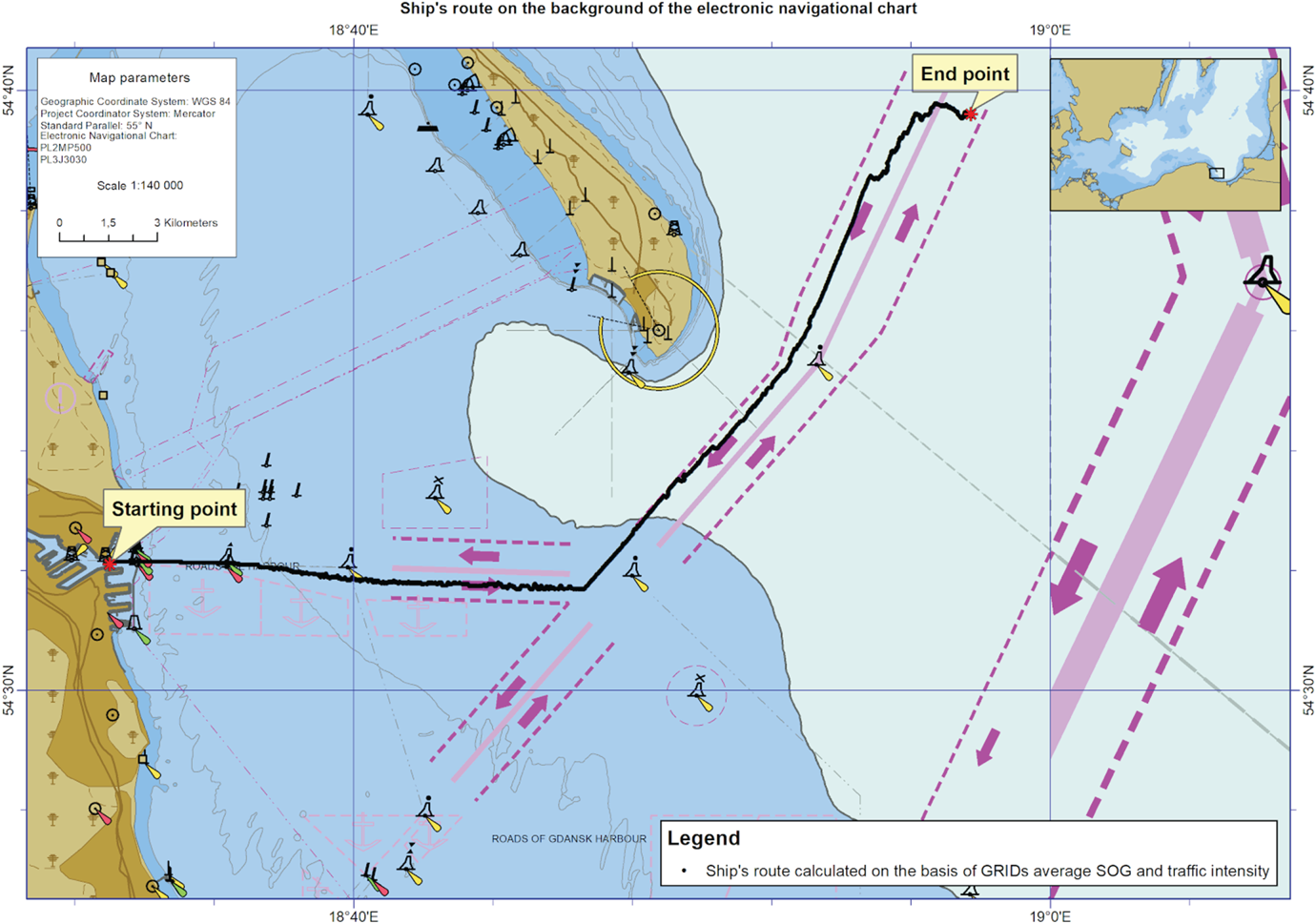
Figure 6. Ship route templates calculated based on GRID average SOG.
In Figures 6–8, set against the electronic navigational chart, ship route map templates are presented calculated separately based on GRID average SOG, GRID average COG and GRID ship traffic intensity based on Function (3).

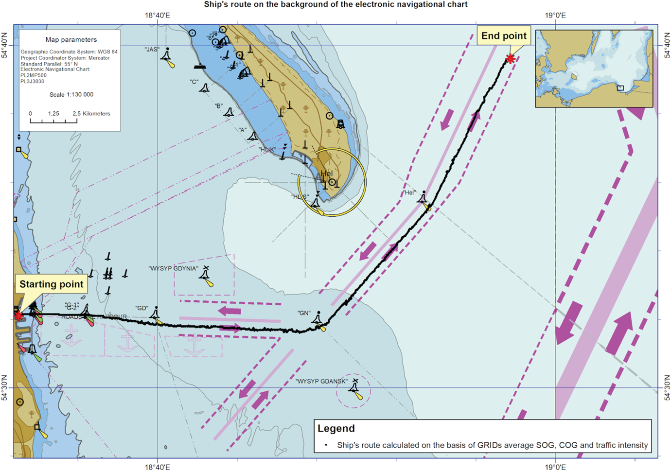
Figure 7. Ship route plan template calculated based on GRID average COG.
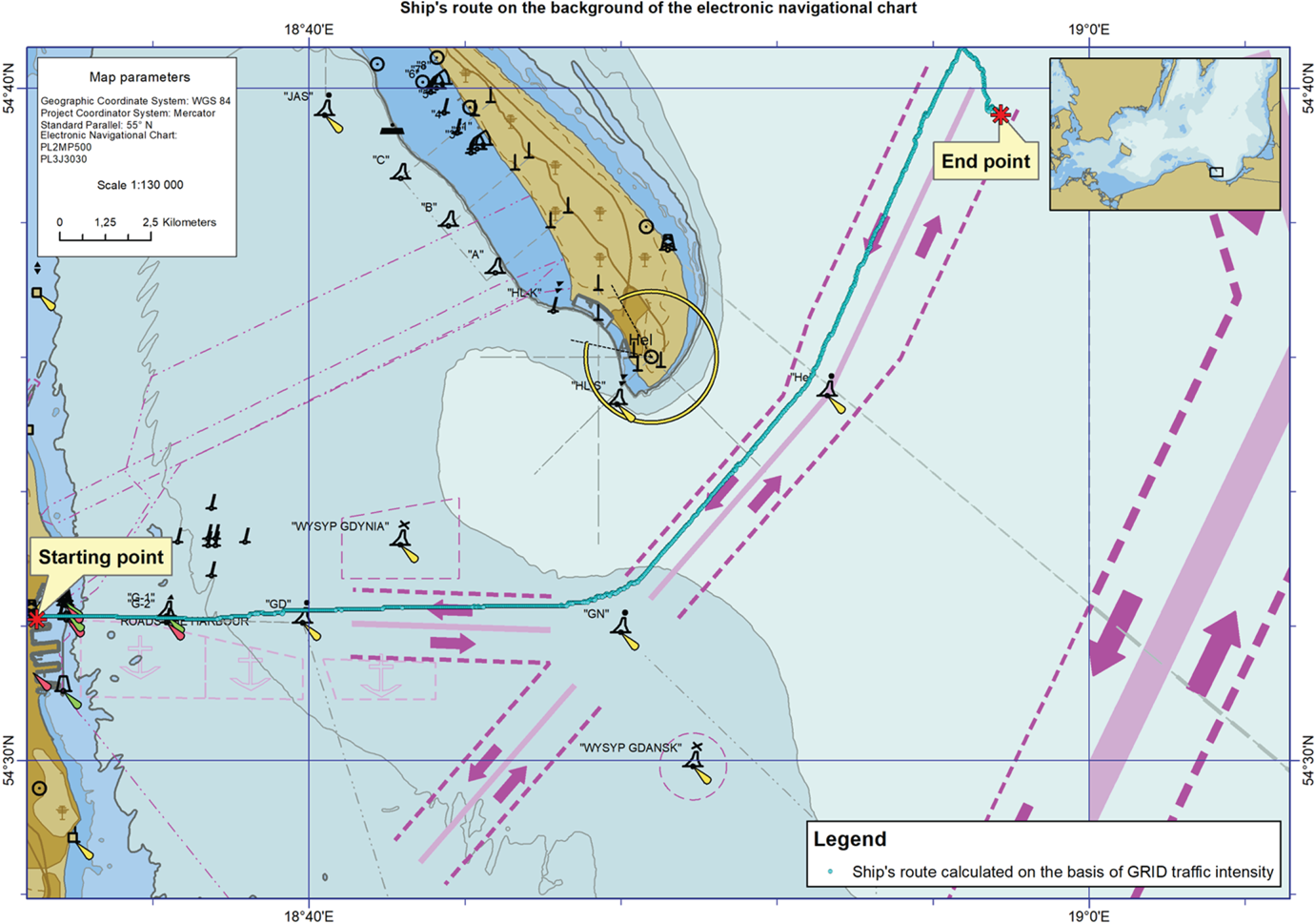
Figure 8. Ship route plan template based on the traffic intensity GRID.
Figure 6 clearly depicts the path of the route plan template (green) calculated on GRID average SOG (as shown in Figure 5) as coinciding with the ships movements on the main fairways. It is comprised of points that have been assigned an average SOG value over 10 knots. In a correct manner, from the north side the ship bypasses three moorings (in an area where the average SOG value does not exceed 2 knots – see Figure 5), but unfortunately, beginning at the ‘GN’ buoy it assumes the wrong fairway, due to the direction of movement (upstream).
The path of the route plan template (yellow) calculated on GRID average COG (as depicted in Figure 4) partially coincides with the streams of ship movements along the main fairways. Unfortunately, its first leg leading eastwards bypasses the main fairways stretching from the ‘GD’ buoy to the ‘GN’ buoy and crosses the mooring area. The second leg, running in a north-eastern direction, can be seen as correct, meaning it follows the direction of movement in the selected fairway.
The path of the route plan template (blue) calculated on the ship traffic intensity GRID (as depicted in Figure 3) runs ideally in the main axes of the ship movement paths, not crossing the lines dividing fairways or bypassing moorings. Unfortunately, almost from the start, it runs in the incorrect fairways considering the direction of movement (upstream).
In Figures 9–11 ship route plan templates are displayed in the background of an electronic navigational map, drafted using Functions (4)–(6), while simultaneously utilising two GRIDs in the following combinations: average SOG and average COG, average COG and ship traffic intensity, and average SOG and ship traffic intensity.

Figure 9. Ship route plan template based on average SOG and average COG GRID.

Figure 10. Ship route plan template based on average COG and the traffic intensity GRID.

Figure 11. Ship route plan template based on average SOG and the traffic intensity GRID.
Unfortunately, as can be seen in Figure 9, the ship route template obtained based on GRID average COG and SOG is not correct. Its first leg is outside the main ship route, running along the main fairway from the port of Gdynia eastward. The second runs along the main fairway, but is designated for ships moving out of the port of Gdañsk. The underlying reason for this outcome is the wrong initial choice of route nodes back at the port. It was primarily influenced by the GRID average SOG nodes, mostly calculated on the high velocity values of the smaller ship moving along the port premises and the route between the port of Gdynia and the port of Gdañsk
The ship route template presented in Figure 10 obtained from GRID average COG and ship traffic intensity had a better initial leg – almost entirely along the exit route from the port of Gdynia. It can clearly be observed that the wrong choice of nodes for the route begins at the very end, in the traffic balancer area. This was definitely caused by the high average COG value, which was mainly influenced by ships bound for the port of Gdañsk and moorings (as shown in the previous example).
The route plan template based on average COG and ship traffic intensity (Figure 10) overlaps with ship traffic streams running along the main fairways, but assumes the wrong direction in its second stage (upstream). It has a similar course as the route presented in Figure 6, the difference being that in this case the values for ship traffic intensity caused the ship route points to move to the fairway axis.
Based on the presented analyses referring to Figures 6–11, the following conclusions can be formulated:
• ship traffic intensity GRID ‘moves’ the route along the main fairways (to be precise in the axes of those fairways, where the traffic intensity is the highest), but it does not consider traffic direction;
• average COG GRID considers the direction, but does not consider the main fairways (combining it with GRID average SOG and GRID ship traffic intensity does not produce satisfactory results);
• average SOG GRID moves the route along the main fairways, but does not consider traffic direction (in this case combining it with GRID traffic intensity does not produce satisfactory results).
These conclusions provided the foundation to formulate function (7) used to simultaneously search through three GRIDs: average SOG, average COG, and ship traffic intensity to draft the route plan template. It was assumed that combining GRID average SOG and ship traffic intensity would improve the precision of ‘placing’ the route plan template along the main fairways, and adding a third GRID average COG would set it in the right direction (by penalising the assumption of a direction not aligned with the average COG).
The path of the route plan template (Figure 12), (black) calculated as a result of browsing three GRID – average SOG, average COG and ship traffic intensity – utilising point evaluation Function (7), can be seen as correct in relation to the current regulations for ships exiting the port of Gdynia and heading north. It runs on the fairways in accordance with their direction of movement. It bypasses moorings, buoys ‘GD’, ‘GN’ and ‘Hel’ on the correct side. Almost in its entirety it is placed on the main axes of fairways, which means that the distance from the fairways' borders is the furthest possible, thus making it the safest.

Figure 12. Ship route plan template based on average SOG, average COG and the traffic intensity GRID.
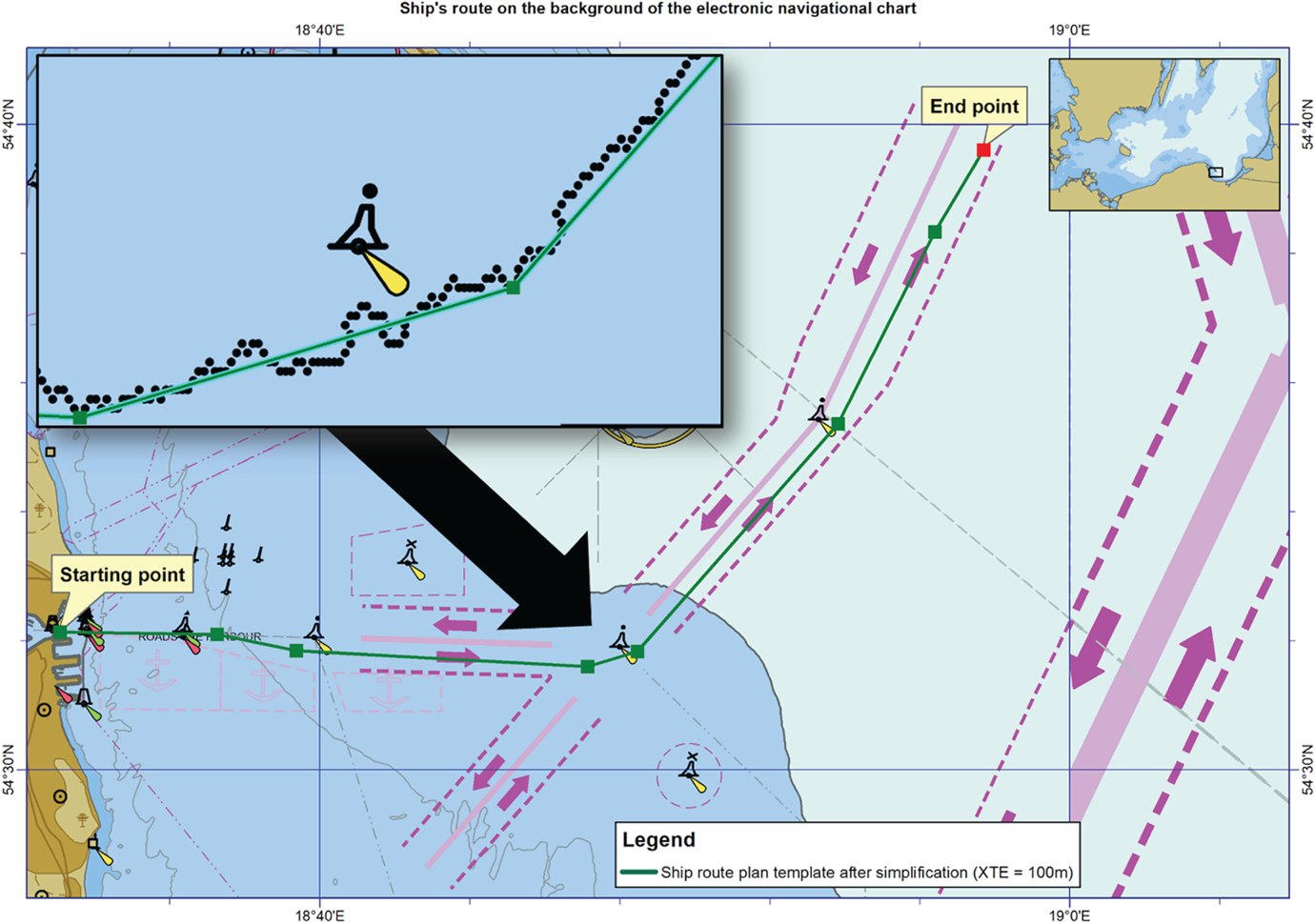
One can note, however, that it consists of a sequence of points that create a very irregular line (with multiple refractions). The line definitely requires smoothing. To that end, the authors proposed using the Douglas–Peucker iterative end-point fit algorithm (Douglas and Peucker, Reference Douglas and Peucker1973; Naus and Wąż, Reference Naus and Wąż2013). The algorithm is based on geometric generalisation from a general perspective (global) – the analysis includes all the points of the model, simplifying each of its consecutive fragments (segments). Two points have to be identified in each iteration: the starting point (‘anchor’), which is established and the target point of the route (‘float’), which is in motion. The first step of the algorithm is to determine a ‘corridor’ interval of tolerance between the anchor and the float). The corridor can be geometrically represented as two parallel lanes with a width corresponding to the cross track error (XTE) located on each side of the segment created by the anchor and the float. The distances perpendicular to all the intermediate points are calculated, starting from the target point and finishing with the point assumed to be the anchor. The sequence of the consecutive intermediate points located within the corridor, created between the anchor and the float (i.e. when their distances perpendicular to the line connecting the float with the anchor are smaller than XTE), is deleted and the float becomes the anchor. The iteration process finishes the moment the anchor reaches the target point. The resulting simplified route consists solely of the points that were qualified as the anchors.
In Figure 13, the route plan template after simplification is presented (the original one was demonstrated in Figure 9).

Figure 13. Ship route plan template after simplification.
3.2. Verification tests
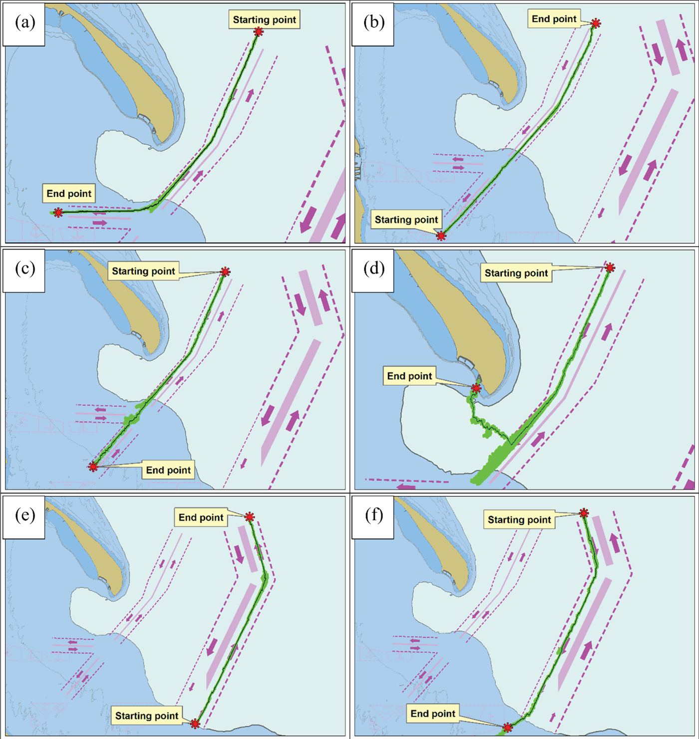
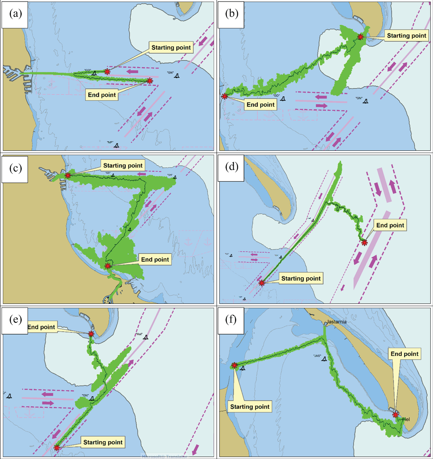
In order to more thoroughly check the developed method in terms of the correctness of searching for points of the path of the route plan template, it was decided to carry out additional simulation tests. The tests were carried out in conditions as close to reality as possible. For this reason, only authorised electronic navigational chart data (coded according to IHO S-57/100 standard, obtained from the Hydrographic Office of the Polish Navy) and actual AIS data collected for a year (recorded according to standard ITU M.1371-5 in daily files with a total size of 15 GB and made available by the Maritime Office in Gdynia) were used in the simulation calculations. Unfortunately, due to the length of time needed to perform a single simulation, essentially consisting in the adequate processing of 15 GB of AIS raw data to find the path of the route plan template for a given start and end point, the tests were limited to 12 representative cases, thus precluding the use of other simulation methods that require a large number of tests to be carried out, for example, the Monte Carlo simulation method. It should be noted that the average time for performing a single trial simulation test was 24 h, despite optimisation of the AIS data processing algorithm and the use of a computer equipped with general-purpose computing on graphics processing units graphic accelerators. Therefore, taking into account the presented limitation and, on the other hand, the need to obtain detailed and reliable verification results for the method conducted in realistic conditions, simulation tests were carried out in two different groups. In the first group, five ‘easy cases’ (a), (b), (c), (e) and (f) (Figure 14) were tested, in which the obtained routes were expected to run on the axes of fairways of traffic separation schemes; and one case that was a bit more complicated, where the route might have intersected with the fairway boundaries heading for the port of Hel (d) (Figure 14). Figure 15 illustrates the second group, where the routes may have intersected with the fairway boundaries or run into areas where there were no fairways. To facilitate the process and to better interpret the results, all the obtained routes were left in their original shape, that is, they were not simplified (in accordance with the algorithm presented in research method section), but presented against the background of the search areas where all the analysed GRID points were located.

Figure 14. The test results of the first group: the route (black); the search area (green).

Figure 15. Test results of the second group: route (black); the search area (green).
Assessing the routes obtained in the first test group, it can be stated that their course was correct. Only in case (d) was the search area considerable, which resulted from the fact that the decision about search direction, under the proposed algorithm (3), depended on weighting distance from the target point d(n, k)/w d, and on the estimated cost calculated in GRID points g s, c, i(n). In this case it can be clearly observed that the search area extended to the intersection of fairways, whereupon the weighting distance reached such a high value that the algorithm made the decision to change the search direction for the port of Hel.
The first case, (a), from the second test group can certainly be assessed as very difficult, because it requires planning a route that crosses over to the neighbouring lane where the traffic is in the opposite direction. In this case the search area correctly moves from the starting point to the port of Gdynia, where it makes a turn and heads for the target point (rightly steering clear of buoy ‘GD’).
In case (b) the search area branches out into two directions, consistent with the directions of standard routes from the port of Hel to the port of Gdynia and to the port of Gdañsk (the movement streams of these routes can be clearly seen in Figures 3–5); however, in the end, the algorithm chooses the route points located in the right direction, though the selected route is irregular in shape.
In Figure 15(c), the largest searched area, a route is presented running between the port of Gdynia and the port of Gdañsk. Initially its search area was heading towards buoy GN, where it should have changed direction towards buoy ‘NP’ (meaning it should have moved on the fairways of the traffic separation scheme). Unfortunately, it changed direction earlier, shortening the length of the route (that is, after the weighting distance from the target reached a high value). A similar situation occurs in cases (d) and (e). The last case (f) presents the route in an area where fairways do not exist. Due to this fact it was created from two customary routes: running towards the port of Jastarnia and then to the port of Hel (the movement streams for those two routes are clearly visible in Figures 3–5).
The obtained test results of led the author conclude that the proposed method is functional for drafting route plan templates running along fairways (that is, when it finds a starting and target point on them). This unfortunately cannot be said about the method when the route plan templates are away from fairways and customary routes; this requires additional, focused research into the method, for example, connected to the use of optimal values of weighting coefficients for d(n, k), g s(n), g c(n), and g i(n) when the route goes beyond the fairway borders.
4. CONCLUSIONS
The obtained research results confirm that it is possible to calculate ship route plan templates based on AIS historical data. Historical AIS data coded in message nos. 1–3 and 18 can be utilised for this purpose. After processing them accordingly, one can obtain a (state) search space described through traffic intensity, average SOG and average COG of the ships' position in a sea area. This area can finally be utilised to calculate paths in ship route plan templates, for example, with the proposed strategy of greedy search. One should realise, however, that such a strategy is not highly effective due to computational complexity, length of time required and the high capacity of computer memory needed. The unquestionable benefits of the proposed solution are as follows.
– The possibility of additionally including up-to-date information pertaining to the limitations and dangers that appear during shipping.
– Gaining the ability to create route plan templates without the necessity of possessing navigational sea maps and nautical publications.
– The ability to calculate route plan templates for specific groups of ships (e.g. divided by types, draught, length or moving with a set speed).
The primary drawback of the method is the fact that it requires the collection and processing of large amounts of AIS data.
The proposed solution is the result of preliminary research, but based on its results, it can be concluded it is worth pursuing this further. The research could be focused on improving its calculational performance, for example, through implementing other methods of discretisation and exploration of search area (sea area described by archived AIS data) or specifying a route plane template in relation to a ship's parameters (draught, length or width).