


1. Introduction
Both the size of an oil droplet and the local flow conditions in the water column combine to control the transport and fate of oil droplets. Large droplets mostly rise faster in the water column due to their higher buoyancy to drag ratio (Zhao et al. Reference Zhao, Boufadel, Adams, Socolofsky, King, Lee and Nedwed2015), and the dissolution and biodegradation rate of oil droplets increases with decreasing droplet size due to larger interfacial area concentration of smaller droplets (Gros et al. Reference Gros, Socolofsky, Dissanayake, Jun, Zhao, Boufadel, Reddy and Arey2017; Socolofsky et al. Reference Socolofsky, Gros, North, Boufadel, Parkerton and Adams2019). At the plume scale, the transport of oil plumes depends on the initial buoyancy flux at the release and the competing effects of density stratification of seawater and horizontal currents (crossflow) in the water column (Boufadel et al. Reference Boufadel, Socolofsky, Katz, Yang, Daskiran and Dewar2020). In this work, the crossflow speed is  $0.51\ \textrm {m}\ \textrm {s}^{-1}$ without stratification and the buoyancy flux has a value of
  $4\times 10^{-3}\ \textrm {m}^{4}\ \textrm {s}^{-3}$ (2.2a–d). Socolofsky, Adams & Sherwood (Reference Socolofsky, Adams and Sherwood2011) reported stratification to be more important in a subsea oil well blowout where the ocean currents are slower than
  $0.1\ \textrm {m}\ \textrm {s}^{-1}$ which was the case in the Deepwater Horizon accident. During the DeepSpill field experiments (Johansen et al. Reference Johansen, Rye, Melbye, Jensen, Serigstad and Knutsen2001), which had high currents and low stratification, the multiphase plume was trapped at heights less than 200 m from the seafloor and transported with ocean currents and droplet buoyancy. The crossflow becomes dominant for numerous situations such as underwater oil leaks in rivers and oil spills in oceans with modest circulation or tidal currents. Crossflow bends a multiphase plume in the horizontal direction; and large oil droplets and gas bubbles separate from the entrained water due to their higher buoyancy to drag ratio (Socolofsky & Adams Reference Socolofsky and Adams2002; Socolofsky, Crounse & Adams Reference Socolofsky, Crounse and Adams2002; Murphy et al. Reference Murphy, Xue, Sampath and Katz2016).
The size of the individual droplets in a crossflow jet depends on jet hydrodynamics near the orifice, but the overall shape of the jet is impacted (in return) by the size of individual droplets, as rising droplets entrain fluid around them. In a prior work (Daskiran et al. Reference Daskiran, Cui, Boufadel, Zhao, Socolofsky, Özgökmen, Robinson and King2020), we found that when using a uniform velocity of droplet rise one could either match the lower or the upper boundary of a crossflow plume, but not both. Therefore, one needs to assign a rise velocity to each computational cell based on the within-cell droplet size distribution to closely capture the hydrodynamics.
The generation of the oil droplet size distribution (DSD) could be conducted using direct numerical simulations (DNS) where the droplet is resolved down to the micron scale. However, this is computationally cost-prohibitive for systems that are metres in scale. For this reason, researchers have relied on using phenomenological models of droplet population (or a population balance model, PBM) to use macroscopic information from the plume (e.g. energy dissipation rate) to produce micron-scale droplets; Pedel et al. (Reference Pedel, Thornock, Smith and Smith2014) used large eddy simulation (LES) to estimate the transport of different-sized coal particles in a jet. However, they did not consider the breakage and aggregation of particles. Aiyer et al. (Reference Aiyer, Yang, Chamecki and Meneveau2019) coupled a PBM with a LES to investigate the DSD from a jet in crossflow to simulate the experiments of Murphy et al. (Reference Murphy, Xue, Sampath and Katz2016). They obtained a good agreement. Their work was first in coupling PBM with LES for a jet in crossflow.
In this work we report experimental results of a large-scale (metres) plume in crossflow from an experiment we conducted at the Ohmsett facility at the Navy Base Earle in New Jersey. We used LES to simulate the macroscopic-scale hydrodynamics, and we coupled the LES to the population model VDROP developed by our group (Zhao et al. Reference Zhao, Torlapati, Boufadel, King, Robinson and Lee2014b). The VDROP model accounts for breakage and coalescence of the dispersed phase (i.e, oil droplets). Recently, Cui et al. (Reference Cui, Daskiran, King, Robinson, Lee, Katz and Boufadel2020a) coupled the VDROP model with a Lagrangian particle tracking model, NEMO3D (Cui et al. Reference Cui, Boufadel, Geng, Gao, Zhao, King and Lee2018) to study the transport of oil droplets under breaking waves using the hydrodynamics obtained from a numerical simulation with  $k-\varepsilon$ turbulence model (Cui et al. Reference Cui, Zhao, Daskiran, King, Lee, Katz and Boufadel2020b).
In § 2 the experimental set-up for the laboratory observations in the Ohmsett tank, including details of the instrumentation, are provided. In § 3 the governing equations are presented. The modifications made to the equations, including the additions of a drift stress term to the momentum equation and adding vertical advection term to the volume fraction equation to represent the influence of the droplet rise velocity on the hydrodynamics, are detailed. The coupling of the VDROP model with LES, and the PBM which is used to compute the breakage source term in the advection–diffusion equations for each size bin are also discussed. The experimental and numerical results are reported in § 4 and the conclusions are presented in § 5.
2. Methods and materials
2.1. Experimental set-up
Large-scale experiments of oil jet were conducted at the Ohmsett tank (www.ohmsett.com) located in Leonardo, New Jersey. The tank dimensions are 203 m (length)  $\times$ 20 m (width)
  $\times$ 2.4 m (depth) and is filled with saltwater with a salinity of around
  $32\ \textrm {g}\ \textrm {l}^{-1}$ mimicking seawater salinity. The tank has two movable bridges with a variable distance between them, and it is capable of towing instruments attached to the bridges at a constant speed. The density and viscosity of the tank water that are slightly higher than the fresh water (Sharqawy, Lienhard & Zubair Reference Sharqawy, Lienhard and Zubair2010) are reported in table 1. The interfacial tension (IFT) between the light crude oil and seawater was reported to decrease with the salinity up to
  ${\sim }200\ \textrm {g}\ \textrm {l}^{-1}$ (Salehi, Omidvar & Naeimi Reference Salehi, Omidvar and Naeimi2017). A decrease in the IFT decreases the resistance of droplets to breakup, thus creating smaller droplets in the system. Fuel oil 2 was used in the experiments, its properties and the IFT between fuel oil and water are reported in table 1.
Table 1. The parameters used in experiment and simulation. The dimensionless numbers are computed based on (2.1a–d), (2.2a–d).

The oil was injected vertically from a pipe 25 mm in diameter and 50 cm tall, suspended from the main bridge and positioned  $\sim$20 cm above the tank bottom (figure 1). Several in-situ instruments were deployed on the auxiliary bridge close to the water surface. During the experiment, both bridges were towed at the same speed along the tank for several minutes at a speed of
  $0.51\ \textrm {m}\ \textrm {s}^{-1}$, which mimicked crossflow. The flow rate of oil was
  $140\ \textrm {l}\ \min ^{-1}$ which resulted in a cross-sectional average vertical velocity of
  $4.75\ \textrm {m}\ \textrm {s}^{-1}$ at the pipe orifice. The jet-to-crossflow velocity ratio,
  $r=U_{j}/U_\infty$, was 9.3 and the jet-to-crossflow momentum ratio,
  $r_m=\rho _{oil}U_{j}^{2}/\rho _{\infty }U_{\infty }^{2}$, was 70. Velocity ratios smaller than 10 represent a strong crossflow situation (Ghosh & Hunt Reference Ghosh and Hunt1998), and has implications on the plume hydrodynamics, such as reduction in the strength of the counter-rotating vortex pair (CVP), discussed below.

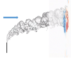
Figure 1. (a) Snapshot of the oil plume during the experiment. The pipe fixed to the main bridge and the frame with instruments fixed to the auxiliary bridge were towed with a speed of  $0.51\ \textrm {m}\ \textrm {s}^{-1}$ from right to left to mimic crossflow from left to right with the same speed. The schematics of the instruments installed on the frame are shown in (b)
  $x$–
$x$– $z$ plane and (c)
  $y$–
$y$– $z$ plane. All scales in (b,c) are in centimetres. (d) The measurement point of ADV below its root is shown in (b,c).
Figure 1(b–d) shows various in-situ instruments employed during the experiments to reveal the hydrodynamics and DSD. The DSD was measured using two shadowgraph cameras (BellaMare, LLC) placed approximately on the same horizontal distance at around 3.75 m (150 diameters) from the orifice (table 2). Each camera consists of an illumination and a telecentric imaging pod facing each other with a gap between them of a few centimetres. The telecentric lenses provide constant droplet size and shape regardless of the droplet distance from the camera within the gap. The images of droplets passing through the gap between illumination and camera pods were captured. The gap can be adjusted based on the concentration of oil to have better images of droplets. It should be large enough to allow the large droplets to pass through with minimal interaction with the camera surfaces and should be small enough to avoid highly concentrated dark images. In the experiments, the gap for the top shadowgraph camera was 34 mm with a field of view of  $65.4\ \textrm {mm} \times 49.1\ \textrm {mm}$, while the gap for the bottom shadowgraph camera was 20 mm with a field of view of
  $33.6\ \textrm {mm}\times 24.6\ \textrm {mm}$. This resulted in a sampling volume of
  $34\ \textrm {mm} \times 65.4\ \textrm {mm} \times 49.1\ \textrm {mm}$ for the top camera and
  $20 \ \textrm {mm}\times 33.6\ \textrm {mm} \times 24.6\ \textrm {mm}$ for the bottom camera. The resolution of the images taken with the top camera was
  $28.1\ \mathrm {\mu }\textrm {m}\ \textrm {pixel}^{-1}$, while it was
  $8.2\ \mathrm {\mu }\textrm {m}\ \textrm {pixel}^{-1}$ for the bottom camera. At least 4 to 5 pixels should cover the apparent droplet diameter to capture the droplet curvature (Shinjo & Umemura Reference Shinjo and Umemura2010; Daskiran et al. Reference Daskiran, Xue, Cui, Katz and Boufadel2021b). Therefore, droplets that were
  $110\ \mathrm {\mu }\textrm {m}$ and larger were considered to be resolved by the top camera, while droplets that were
  $35 \ \mathrm {\mu }\textrm {m}$ and larger were considered to be resolved by the bottom camera. Pictures were taken at 26 frames per second (f.p.s.) by the top camera and 9 f.p.s. by the bottom camera. Images from the shadowgraph cameras were analysed using the software ImageJ (Rasband Reference Rasband1997–2016) to obtain the largest cross-sectional area of individual droplets.
Table 2. Position of the shadowgraph cameras with respect to the centre of the pipe orifice. The crossflow is in the  $x$-direction, the jet is released
  $90^{\circ }$ to the crossflow in the
  $z$-direction.

The Reynolds number (Re) based on oil velocity at the orifice and pipe diameter, Weber number (We), Ohnesorge number (Oh) and Froude number (Fr) are computed as
 \begin{align} Re=\frac{\rho_{oil}U_{j}D}{\mu_{oil}};\quad {We}=\frac{\rho_{oil}U_{j}^{2}D}{\sigma};\quad {Oh}=\frac{\sqrt{{We}}}{Re}=\frac{\mu_{oil}}{\sqrt{\rho_{oil}\sigma{D}}} ;\quad \textit{Fr}=\frac{U_j}{\sqrt{g^{\prime}D}}.\end{align}
Here,  $U_{j}$ is the average jet velocity inside the pipe,
  $\rho _{oil}$ is the oil density,
  $\rho _\infty$ is the continuous fluid (i.e. sea water) density,
  $\mu _{oil}$ is the dynamic viscosity of oil,
  $\sigma$ is the IFT coefficient between oil and water and
  $g^{\prime }=(({\rho _{\infty }-\rho _{oil})}/{\rho _{\infty }})g$ is the reduced acceleration of gravity. The values of the non-dimensional numbers are given in table 1. Based on the Oh vs Re diagram (Johansen, Brandvik & Farooq Reference Johansen, Brandvik and Farooq2013; Zhao et al. Reference Zhao, Boufadel, Adams, Socolofsky, King, Lee and Nedwed2015), droplet breakup at the orifice was found to be in the atomization regime, a regime well simulated by the VDROP model.
Several length scales (Wright Reference Wright1977; Jirka & Domeker Reference Jirka and Domeker1991; Jirka Reference Jirka2004) are invoked herein since we will be comparing our numerical results to Jirka's integral model. The discharge length scale  $L_Q$, the jet-to-crossflow transition length scale
  $L_m$, the plume-to-crossflow transition length scale
  $L_b$ and the jet-to-plume transition length scale
  $L_M$ are given by
 \begin{equation} L_Q=\frac{Q_o}{\sqrt{M_o}};\quad L_m=\frac{\sqrt{M_o}}{U_\infty};\quad L_b=\frac{J_o}{U_\infty^{3}};\quad L_M=\frac{M_o^{3/4}}{\sqrt{J_o}} . \end{equation}
Here,  $Q_o=U_ja_o$ is the volumetric flux and
  $a_o$ is the cross-sectional area of the pipe,
  $M_o=U_j^{2}a_o$ is the momentum flux and
  $J_o=U_ja_og^{\prime }$ is the buoyancy flux. The values of length scales are reported in table 1.
3. Mathematical modelling and numerical approach
3.1. Governing equations – LES
In this study a single continuity and momentum equations are solved for the mixture, and the phases share the same velocity in the horizontal and lateral directions while the rise velocity of oil droplets is considered in the vertical direction (Fabregat Tomàs et al. Reference Fabregat Tomàs, Poje, Özgökmen and Dewar2016). To account for the rise velocity of oil droplets, a drift stress term was added to the momentum equation (Manninen, Taivassalo & Kallio Reference Manninen, Taivassalo and Kallio1996; Fabregat Tomàs et al. Reference Fabregat Tomàs, Poje, Özgökmen and Dewar2016) and an additional advection term was added to the volume fraction equation (Fabregat Tomàs et al. Reference Fabregat Tomàs, Poje, Özgökmen and Dewar2016; Yang et al. Reference Yang, Chen, Socolofsky, Chamecki and Meneveau2016), both as a function of the slip velocity of droplets.
A transport equation for the volume fraction was solved to predict the spatial and temporal distribution of the two phases (oil and water). Although the original form of the model was based on the VOF model (Hirt & Nichols Reference Hirt and Nichols1981; Milanovic, Zaman & Bencic Reference Milanovic, Zaman and Bencic2012) in which phases share the same velocity field, the usage of the slip velocity among the phases renders the model used herein to be the mixture model (Manninen et al. Reference Manninen, Taivassalo and Kallio1996; Fabregat Tomàs et al. Reference Fabregat Tomàs, Poje, Özgökmen and Dewar2016). In contrast to the works by Yang et al. (Reference Yang, Chen, Socolofsky, Chamecki and Meneveau2016) and Aiyer et al. (Reference Aiyer, Yang, Chamecki and Meneveau2019), the IFT forces and the drift stress term which is a function of individual droplet rise velocity were considered in the momentum equation in this work.
The turbulent flow was modelled using a LES turbulence model (Yuan, Street & Ferziger Reference Yuan, Street and Ferziger1999; Bodart et al. Reference Bodart, Coletti, Bermejo-Moreno and Eaton2013; Galeazzo et al. Reference Galeazzo, Donnert, Cárdenas, Sedlmaier, Habisreuther, Zarzalis, Beck and Krebs2013; Ruiz, Lacaze & Oefelein Reference Ruiz, Lacaze and Oefelein2015; Ryan et al. Reference Ryan, Bodart, Folkersma, Elkins and Eaton2017) in which eddies larger than the filter size are resolved and the smaller ones are modelled through subgrid scale (SGS) models. The filtered form of the Navier–Stokes equations is given as
 $$\begin{gather} \boldsymbol{\nabla}\boldsymbol{\cdot}({\rho_m\boldsymbol{u}})=0, \end{gather}$$
 $$\begin{gather}\frac{\partial(\rho_m\boldsymbol{u})}{\partial{t}}+\boldsymbol{\nabla}\boldsymbol {\cdot} (\rho_m\boldsymbol{u}\boldsymbol{u})={-}\boldsymbol{\nabla}{p_{rgh}}+\boldsymbol{\nabla}\boldsymbol{\cdot}{{\boldsymbol{\tau}}_{ \mu_m}}-\boldsymbol{\nabla}\boldsymbol{\cdot}({\rho_m{\boldsymbol{\tau}}^{r}})+ \boldsymbol{\nabla}\boldsymbol{\cdot}{{\boldsymbol{\tau}}_{dm}}+F_{st}-\boldsymbol{g}\boldsymbol{\cdot}\boldsymbol{x}{\boldsymbol{\nabla} }{\rho_m}. \end{gather}$$
Here,  $\boldsymbol {u}$ is the mixture velocity resolved by LES,
  $p_{rgh}$ is the resolved pressure excluding hydrostatic pressure,
  $\rho _m$ is the mixture density,
  $\boldsymbol {x}$ is the position vector and
  $\boldsymbol {\tau }_{\mu _m}=2{\mu _m}\boldsymbol{\mathsf{S}}_{ij}$, where
  $\mu _m$ is the dynamic viscosity of the mixture and
  $\boldsymbol{\mathsf{S}}_{ij}=\frac {1}{2}({\partial {u_i}}/{\partial {x_j}}+{\partial {u_j}}/{\partial {x_i}})$ is the strain-rate tensor. The mixture density and dynamic viscosity were computed using the phase volume fraction as follows:
 \begin{equation} \rho_m=\rho_d\alpha_d+\rho_c(1-\alpha_d);\quad \mu_m=\mu_d\alpha_d+\mu_c(1-\alpha_d). \end{equation}
Here, the subscripts  $d$ and
  $c$ represent the dispersed (oil) and continuous (water) phases, respectively. Note that
  $\alpha _d+\alpha _c=1.0$.
The external force term  $F_{st}=\sigma \kappa \boldsymbol {\nabla }\alpha _d$ represents the surface tension forces between the two phases, where
  $\kappa$ is the interface curvature evaluated based on local surface normal. It was modelled herein using the continuum surface force (CSF) approach by Brackbill, Kothe & Zemach (Reference Brackbill, Kothe and Zemach1992), compared with other approaches by Popinet (Reference Popinet2018). The CSF approach converts the surface forces to volume forces using Green's theorem (Francois, Sicilian & Kothe Reference Francois, Sicilian and Kothe2007). In contrast to single-phase LES, additional unclosed SGS terms including diffusive, temporal, surface tension and interfacial terms appear in the filtered form of the multifluid/multiphase LES equations (Saeedipour & Schneiderbauer Reference Saeedipour and Schneiderbauer2019). The surface tension SGS term was the subject of several studies in the recent decade (Herrmann Reference Herrmann2010; Liovic & Lakehal Reference Liovic and Lakehal2012; Saeedipour & Schneiderbauer Reference Saeedipour and Schneiderbauer2019; Hasslberger, Ketterl & Klein Reference Hasslberger, Ketterl and Klein2020) that investigate the effect of SGS surface tension force on the interfacial flows through different approaches. The subgrid contribution of surface tension force is considered to be proportional to the resolved surface tension force as (Shirani, Jafari & Ashgriz Reference Shirani, Jafari and Ashgriz2006; Saeedipour & Schneiderbauer Reference Saeedipour and Schneiderbauer2019; Hasslberger et al. Reference Hasslberger, Ketterl and Klein2020)
 \begin{equation} {F_{st}^{r}=C_{st}\left(\frac{\nu_{SGS}}{\nu_m}\right)^{1/2}F_{st}} , \end{equation}
where  $\nu _{SGS}$ is the subgrid eddy viscosity and
  $C_{st}$ is an empirically determined constant (Hasslberger et al. Reference Hasslberger, Ketterl and Klein2020). There is not a well-established value for
  $C_{st}$ in the literature. Moreover, the approach of incorporating subgrid surface tension still requires an extension to three dimensions and still requires a close validation.
The SGS stress tensor,  $\boldsymbol {\tau }_{ij}^{r}= \widetilde {\boldsymbol {u}_{\boldsymbol {i}}\boldsymbol {u}_{\boldsymbol {j}}}- \widetilde {\boldsymbol {u_i}}\widetilde {\boldsymbol {u_j}}$, which appears due to the filtering operation was computed through SGS modelling. The deviatoric part of SGS stress,
  $\boldsymbol {\tau }_{ij}^{r}-\frac {1}{3}\boldsymbol {\tau }_{kk}^{r}\delta _{ij}$, was modelled following the Boussinesq hypothesis (Pope Reference Pope2000)
 \begin{equation} \boldsymbol{\tau}_{\boldsymbol{ij}}^{\boldsymbol{r}}-\tfrac{1}{3}\boldsymbol{\tau}_{kk}^{r}\delta_{ij}={-}2\nu_{SGS} \boldsymbol{\mathsf{S}}_{ij}, \end{equation}
where  $\boldsymbol {\tau }_{kk}^{r}$ is the isotropic part of the SGS stress which is added to the filtered pressure,
  $\delta _{ij}$ is the Kronecker delta. In this work the Smagorinsky SGS model was employed to predict SGS eddy viscosity, given by
 \begin{equation} \nu_{SGS}=(C_s\varDelta)^{2}|\boldsymbol{\mathsf{S}}|, \end{equation}
where  $|\boldsymbol{\mathsf{S}}|=\sqrt {2\boldsymbol{\mathsf{S}}_{ij}\boldsymbol{\mathsf{S}}_{ij}}$ and
  $C_s$ is the Smagorinsky constant taken as 0.168 in the present study and
  $\varDelta$ is the filter size which is computed as
  $\forall ^{1/3}$, where
  $\forall$ is the cell volume.
Jones & Wille (Reference Jones and Wille1996) compared the experimental measurements of Chen & Hwang (Reference Chen and Hwang1991) for a planar jet in crossflow against their LES with SGS models including the standard Smagorinsky model (used herein), the dynamic Smagorinsky model (Piomelli & Liu Reference Piomelli and Liu1995) and the one-equation (subgrid kinetic energy equation,  $k_{SGS}$) model (Yoshizawa Reference Yoshizawa1986). They found based on the comparison of mean axial velocity and axial turbulent intensity
  $u^{\prime } / U_{max}$ that the one-equation and dynamic models provided slightly improved predictions. For a free jet, Yu, Luo & Girimaji (Reference Yu, Luo and Girimaji2006) compared the streamwise velocity profiles and decay of the centreline velocity obtained from their LES with the standard Smagorinsky model to the measurements of Quinn & Militzer (Reference Quinn and Militzer1988) and found a good agreement. For these reasons, we adopted the standard Smagorinsky model herein. We are cognizant that the dynamic SGS model (Yuan et al. Reference Yuan, Street and Ferziger1999; Yang et al. Reference Yang, Chen, Socolofsky, Chamecki and Meneveau2016; Aiyer et al. Reference Aiyer, Yang, Chamecki and Meneveau2019) is likely to be an improvement over the standard one, but we believe the difference in the SGS model is small for the current work.
The drift stress term,  $\boldsymbol {\tau }_{dm}$, appears in the momentum equation as a result of the slip velocity between the phases. It was computed as
 \begin{equation} \boldsymbol{\tau}_{dm}={-}\sum_{k=1}^{N}\alpha_k\rho_k\boldsymbol{u}_{dr,k}\boldsymbol{u}_{dr,k}, \end{equation}
where  $N$ is the number of phases,
  $\boldsymbol {u}_{dr,k}$ is the drift velocity of phase
  $k$ which is defined as the difference between the phase velocity and the mixture velocity,
  $\boldsymbol {u}_{dr,k}=\boldsymbol {u}_k-\boldsymbol {u}_m$, where
  $\boldsymbol {u}_m=\sum _{k=1}^{N}c_k\boldsymbol {u}_{k}$. The term
  $c_k$ is the mass fraction of the dispersed phase (i.e. oil) which is computed as
  $c_k={\alpha _k\rho _k}/{\rho _m}$. The drift velocity of a dispersed phase can be presented in terms of relative velocities as (Manninen et al. Reference Manninen, Taivassalo and Kallio1996; Kruskopf Reference Kruskopf2017)
 \begin{equation} \boldsymbol{u}_{dr,k}=\boldsymbol{u}_{ck}-\sum_{l=1}^{N}c_l\boldsymbol{u}_{cl}, \end{equation}
where  $\boldsymbol {u}_{ck}=u_k-u_c$ and the subscript
  $c$ represents the continuous phase. After computing the drift velocities for the continuous and dispersed phases from (3.8), the drift stress term in (3.7) can be written as
 \begin{equation} \boldsymbol{\tau}_{dm}={-}\rho_mc_d(1-c_d)u_{cd}u_{cd}. \end{equation}
 The slip velocity of the dispersed oil phase was assumed to be only in the vertical direction and, hence,  $\boldsymbol {u}_{cd}=w_r{\boldsymbol {e}_{\boldsymbol {3}}}$, where subscript
  $d$ represents the dispersed phase. The slip velocity,
  $w_r$, was computed based on the mass-weighted average of the rise velocities of different-sized droplets at each cell in the computation domain, which will be given later (3.16). The drift stress term affects the vertical momentum of the mixture based on the local average rise velocity of droplets which accounts for the rise velocity of different-sized droplets.
The slip velocity was included in the volume fraction equation as follows (Manninen et al. Reference Manninen, Taivassalo and Kallio1996):
 \begin{equation} \frac{\partial{\alpha_d}}{\partial{t}}+\boldsymbol{\nabla}\boldsymbol{\cdot}(\alpha_d\boldsymbol{u})={-}\frac{\partial{ [\alpha_d(1-c_d)w_r{\boldsymbol{e}_{\boldsymbol{3}}}]}}{\partial{z}} . \end{equation}
Here, the term on the right-hand side represents the advection term induced by the mass-weighted average slip velocity of the oil phase where  $\boldsymbol {e}_{\boldsymbol {3}}$ is the unit vector in the
  $z$-direction (vertical).
3.2. Advection–diffusion equations – droplet transport
The transport equations of the number concentration of droplets are solved for each size bin to track the evolution of the droplet size in the flow field. In the transport equations, the advection and diffusion of droplets, the slip velocity of droplets with diameter  $d_{i}$ and the source terms for droplet breakage and coalescence are considered as follows (Fabregat Tomàs et al. Reference Fabregat Tomàs, Poje, Özgökmen and Dewar2016; Yang et al. Reference Yang, Chen, Socolofsky, Chamecki and Meneveau2016):
 \begin{align} &\frac{\partial{n(d_i,{{\boldsymbol{x}}},t)}}{\partial{t}}+\boldsymbol{\nabla} \boldsymbol{\cdot}[\boldsymbol{u}({{\boldsymbol{x}}},t)n(d_i,{{\boldsymbol{x}}},t))]- \boldsymbol{\nabla}^{2}[(D_b+D_{SGS})n(d_i,{{\boldsymbol{x}}},t)]\nonumber\\ &\quad +w_{r,i}{\boldsymbol{e}_{\boldsymbol{3}}}\frac{\partial{n(d_i,{{\boldsymbol{x}}},t)}}{\partial{z}}=S_{b,i}+S_{c,i} . \end{align}
Here  $n(d_i,{{\boldsymbol {x}}},t)$ is the number concentration of droplets (number of
  $\textrm {droplets}\ \textrm {m}^{-3}$) with diameter
  $d_i$ at a given time (
 $t$) and position (
 ${{\boldsymbol {x}}}$ vector). The second term on the left-hand side represents the advection of droplets with the mixture velocity. The third term on the right-hand side represents the diffusion of oil in water which is induced by the gradient of the number concentration of the size bin. The molecular diffusion coefficient of oil in water
  $D_b$ at
  $20^{\circ }$ was taken to be 1.12
 $\times 10^{-8}\ \textrm {m}^{2}\ \textrm {s}^{-1}$ (Hamam Reference Hamam1987). It is a small value at the time scale of our work, but it is kept herein for completeness. The SGS diffusion coefficient
  $D_{SGS}$ was computed based on the subgrid Schmidt number (
 $Sc_{SGS}=1.0$) and the subgrid eddy viscosity
  $\nu _{SGS}$ in (3.6). The fourth term represents the rise of droplets due to the slip velocity. The terms
  $S_{b,i}$ and
  $S_{c,i}$ are the breakage and coalescence terms of the droplets with diameter
  $d_{i}$. The coalescence was considered to be negligible due to the small volume fraction of the dispersed oil phase beyond 10 diameters from the release (Boufadel et al. Reference Boufadel, Socolofsky, Katz, Yang, Daskiran and Dewar2020). This was also adopted by Aiyer et al. (Reference Aiyer, Yang, Chamecki and Meneveau2019) who coupled a PBM to LES. The breakage term was computed using the VDROP population model (Zhao et al. Reference Zhao, Boufadel, Socolofsky, Adams, King and Lee2014a) and was provided to (3.11). The terminal rise (slip) velocity of droplets of diameter
  $d_{i}$ is given by White & Corfield (Reference White and Corfield2006) and Zhao et al. (Reference Zhao, Boufadel, Adams, Socolofsky, King, Lee and Nedwed2015), i.e.
 \begin{equation} w_{r,i}=\sqrt{\frac{4gd_i(\rho_c-\rho_d)}{3C_{D,i}\rho_c}}, \end{equation}
where the term  $C_{D,i}$ is the drag coefficient of droplets with diameter
  $d_{i}$ which can be estimated using the Schiller–Naumann drag coefficient model (Naumann & Schiller Reference Naumann and Schiller1935), given by
 \begin{equation}
C_{D,i}=\left\{\begin{array}{@{}ll}
\dfrac{24(1+0.15Re_{d,i}^{0.687})}{Re_{d,i}}, &
Re_{d,i}\leqslant 1000, \\ 0.44, &
Re_{d,i}>1000.
\end{array}\right. \end{equation}
\begin{equation}
C_{D,i}=\left\{\begin{array}{@{}ll}
\dfrac{24(1+0.15Re_{d,i}^{0.687})}{Re_{d,i}}, &
Re_{d,i}\leqslant 1000, \\ 0.44, &
Re_{d,i}>1000.
\end{array}\right. \end{equation}
The Reynolds number of droplets with diameter  $d_{i}$ in the equation above is defined as
 \begin{equation} Re_{d,i}=\frac{\rho_cw_{r,i}d_i}{\mu_c}. \end{equation}
Equation (3.12) is a good predictor for the terminal velocity for the maximum size of droplets considered in this work, which is 3.7 mm. The equation might not be appropriate for much larger droplets (e.g. 8 mm), where the droplet is oblate, and empirical equations based on experimental results would need to be used (Zheng & Yapa Reference Zheng and Yapa2000; Clift, Grace & Weber Reference Clift, Grace and Weber2005; Zhao et al. Reference Zhao, Boufadel, Lee, King, Loney and Geng2016).
The number concentration equation (3.11) was solved for 14 bin sizes starting from  $d_{1}=100\ {\mathrm {\mu }}\textrm {m}$ up to
  $d_{14}=3.7\ \textrm {mm}$. The droplet size at the maximum size bin (i.e.
  $d_{14}$) was determined based on the maximum droplet size measured at the top camera in our experiments. The size bins are discretized logarithmically based on the relation
 \begin{equation} d_{i+1}=2^{k}d_i,\quad \textrm{where}\ i=1,2,\ldots,14\quad \textrm{and}\quad k=0.4. \end{equation}
 In the interpretation of the experimental results, the lower and upper boundary of each bin was defined as  $d_{i-1/2}=2^{-k/2}d_i$ and
  $d_{i+1/2}=2^{k/2}d_i$, respectively. For instance, the first bin (
 $d_{1}=100\ \mathrm {\mu }\textrm {m}$) in the experiment includes droplets in the range from
  $d_{i-1/2}=87\ \mathrm {\mu }\textrm {m}$ to
  $d_{i+1/2}=115\ \mathrm {\mu }\textrm {m}$, ensuring the volumetric median of the lower and upper boundary of the bin gives the bin size as
  $d_i=\sqrt {d_{i-1/2}d_{i+1/2}}$ (i.e.
  $100\ \mathrm {\mu }\textrm {m}$).
As mentioned earlier, the rise velocity of the oil phase in (3.9), (3.10) is computed after each time step based on the mass-weighted average rise velocity of droplets in various sizes at each cell as follows:
 \begin{equation} w_r({{\boldsymbol{x}}},t)=\frac{\displaystyle\sum_{i=1}^{N_d}n(d_i,{{\boldsymbol{x}}},t) m_iw_{r,i}}{\displaystyle\sum_{i=1}^{N_d}n(d_i,{{\boldsymbol{x}}},t)m_i}. \end{equation}
Here,  $N_{d}$ represents the number of bins and
  $m_i$ is the mass of a single droplet with diameter
  $d_{i}$ which can be replaced with the volume of a single droplet with diameter
  $d_{i}$ since the oil density is constant.
3.3. Simulation set-up
Figure 2 shows the general simulation set-up. The distance from the crossflow inlet to the vertical pipe where the jet was released was 120 $D$ while the domain outlet was placed 240
 $D$ away from the pipe. The distance from the orifice to the camera was around 150
 $D$ (table 2), and the closet instrument (i.e. bottom camera) to the outlet (one the right) was more than 80
 $D$. The distance between the orifice and the water surface was 68
 $D$, and was adopted for the simulation. The water surface was assumed immobile with zero shear wall boundary condition.

Figure 2. (a) Side and front (looking downstream) view of the computational domain with geometric details used in the simulation. The pipe internal diameter is 25 mm and the pipe length is  $20D$. The pipe is
  $8D$ above the tank bottom. Instantaneous isosurface of oil volume fraction at 0.001 from the simulation with
  $K_b=0.05$ is shown. Note that the sketches were not drawn to scale.
At the inlet of the pipe, a velocity of  $4.75\ \textrm {m}\ \textrm {s}^{-1}$ with a top-hat profile (i.e, uniform value) was adopted. The profile becomes sheared at the orifice (exit from the pipe). For the initial size of droplets, we adopted a uniform value equal to maximum droplet size measured by the cameras (i.e. 3.7 mm), as pursued by Aiyer et al. (Reference Aiyer, Yang, Chamecki and Meneveau2019). The number concentration of the 3.7 mm droplets was computed as
 \begin{equation} n_{orifice}=\frac{\varphi}{{\rm \pi} d_o^{3}/6} , \end{equation}
where  $\varphi$ is the oil volume fraction at the orifice which is unity and
  $d_o$ is the droplet size at the orifice (
 $d_{o}=3.7\ \textrm {mm}$). The number concentration at the orifice (
 $n_{orifice}$) was thus
  $3.77\times 10^{7}\ \textrm {m}^{-3}$.
A uniform water velocity profile with  $0.51\ \textrm {m}\ \textrm {s}^{-1}$ speed was assigned for the crossflow inlet, which was intended to simulate that the plume which is 28
 $D$ (0.7 m) above the bottom boundary experienced almost uniform crossflow velocity. During the towing in nearly stationary water in the experiments, the leading edge of the jet and the upper boundary of the plume were exposed to nearly no-perturbed flow which was taken into account in the simulation by adopting no-perturbation at the crossflow inlet. A constant gauge pressure of 0 Pa was assigned on the outlet along with a zero-gradient velocity normal to the outlet surface. The inner and outer surfaces of the pipe and the bottom surface of the tank were considered as wall with a no-slip condition. A zero-shear (free-slip) boundary condition was applied at the domain side boundaries (i.e. parallel to crossflow) and at the water surface. Initially, the pipe was considered to be filled with oil with a top-hat velocity profile.
In the DNS of Muppidi & Mahesh (Reference Muppidi and Mahesh2007) for a jet in a crossflow with a  $Re=5000$, 11 million cells were used. On the pipe inlet face, they adopted structured mesh with
  $0.025D$ cell size in the tangential direction and
  ${\sim }0.01D$ in the radial direction. This face mesh was swept in the vertical direction inside the pipe using cells with an edge length of
  $0.02D$. A cell size of
  $0.1 - 0.15D$ was used in the region of interest (
 $5D$ on either side of the symmetry plane and up to
  $20D$ downstream of the jet exit) at
  $z/D=0$ plane. The mesh on the
  $z/D=0$ plane was swept in the
  $z$-direction with a cell size of
  $0.1D$ outside of the crossflow boundary layer up to
  $z/D\approx 28$ above which the cell size increased linearly at a rate of 1.1. Cintolesi, Petronio & Armenio (Reference Cintolesi, Petronio and Armenio2019) conducted LES of a buoyant jet in crossflow with the jet Reynolds number of 8,200. They adopted a cell size of
  $0.2D$ near the orifice,
  $0.25D$ about the orifice in a rectangular region with
  $28D$,
  $30D$ and
  $6D$ dimensions in the
  $x$,
$x$,  $z$ and
  $y$ directions and a coarser mesh elsewhere with a cell size of
  ${\sim }0.5D$. In the LES work of Galeazzo et al. (Reference Galeazzo, Donnert, Cárdenas, Sedlmaier, Habisreuther, Zarzalis, Beck and Krebs2013) for a jet in crossflow with
  $Re=19\,200$, they used tetrahedral mesh elements in the whole domain (except the hexahedral wall-normal mesh elements) with an edge length of
  $0.025D$ in the near field (
 $x/D<4$) and
  $0.125D$ in the far field (
 $x/D>4$).
In this work mostly structured and hexahedral mesh elements were used to discretize the whole domain. The domain was split into subdomains with the larger cell size outside the plume and near the channel boundaries. The subdomains were coupled using non-conformal mesh interfaces. The region occupied by the oil plume which we know from the snapshots in the experiment (figure 1) was discretized using finer mesh. The cell size increased along the jet path (i.e.  $s$-direction) and outside the plume. The cell size inside the pipe and at the pipe orifice was around
  $0.02D$ and
  $0.024D$ in the radial and tangential direction, respectively. The cell size in the
  $z$-direction was
  ${\sim }0.04D$ near the pipe orifice. Above the orifice along the jet path, the cell size in the tangential direction was
  ${\sim }1.2$ times larger than that in the radial direction. At
  $s/D\approx 10$, the cell size was
  $0.18D$ in the radial direction and
  $0.13D$ in the jet direction. The fine mesh region was expanded in the radial direction while moving downstream due to the radial expansion of the jet. At
  $s/D\approx 23$, the cell size increased to
  $0.3D$ in the radial direction and to
  $0.2D$ in the jet direction. At
  $s/D\approx 55$, the cell size increased to
  $0.56D$ in the radial direction and to
  $0.26D$ in the jet direction. The increase in the cell size along the jet direction was slower after
  $s/D\approx 50$. At
  $s/D\approx 100$, the cell size increased to
  $0.74D$ in the radial direction and to
  $0.27D$ in the jet direction. At
  $s/D\approx 140$, the cell size in the radial direction increased to
  $0.83D$ while the cell size in the tangential direction remained the same. The mesh was coarsened outside the region of interest (i.e. the plume region) gradually to reach a uniform cell size of
  $2.6D$ in all directions. A large uniform cell size of
  $4.2D$ was adopted near the domain side boundaries which started
  $50D$ away from the jet centre plane. The time step size used in the simulation was
  ${\sim }1\times 10^{-3}$ characteristic time units (
 $D/U_\infty$) for the mesh with 5.8 million cells and
  ${\sim }6.1\times 10^{-4}$ characteristic time units for the mesh with 10.6 million cells. The time averaging was started at
  $t=9.6\ \textrm {s}$ (197 time units) after the flow passed the location of the cameras used in the experiments. The time averaging was performed over 76 other time units from 9.6 s to 13.3 s.
3.4. Population balance model – VDROP
The VDROP model is a discrete population model which considers both dispersed phase viscosity and IFT as a breakup resistance force, together with VDROP-J, the model was validated using over 40 datasets and, hence, provides a realistic DSD (Zhao et al. Reference Zhao, Boufadel, Socolofsky, Adams, King and Lee2014a,Reference Zhao, Torlapati, Boufadel, King, Robinson and Leeb). Considering only droplet breakup (i.e. neglecting droplet coalescence), the number concentration of droplets of size  $d_i$,
  $n(d_i,t)$ evolves as
 \begin{equation} \frac{\partial n(d_i,t)}{\partial t}={-}g(d_i)n(d_i,t)+\sum_{j=i+1}^{N_d}\beta(d_i,d_j)g(d_j)n(d_j,t), \end{equation}
where  $n(d_i,t)$ is the number concentration (number of
  $\textrm {droplets}\ \textrm {m}^{-3}$) of droplets with diameter
  $d_i$ in metres at a given time
  $t$ (s). The function
  $g(d_i)$ is the breakage frequency of droplets with diameter
  $d_i$ (reported below). The first term on the right-hand side of (3.18) represents the death of droplets with size
  $d_i$. The term
  $\beta (d_i,d_j)$ is the breakage probability density function (dimensionless) for the creation of droplets with diameter
  $d_i$ due to breakage of droplets with (a larger) diameter
  $d_j$ (Tsouris & Tavlarides Reference Tsouris and Tavlarides1994). It represents the fact that the probability of the droplet breakage into two unequal-sized daughter droplets is higher since the breakage into droplets with equal sizes requires more energy. The second term on the right-hand side of (3.18) represents the birth of droplets
  $d_i$ resulting from the breakup of droplets of size
  $d_j$ larger than
  $d_i$. The breakage rate
  $g(d_i)$ can be expressed as (Tsouris & Tavlarides Reference Tsouris and Tavlarides1994)
 \begin{equation} g(d_i)=K_b\int_{n_e}S_{ed}(u_e^{2}+u_d^{2})^{1/2}BE(d_i,d_e,\varepsilon,t)\,\textrm{d}n_e, \end{equation}
where  $K_b$ is a system-dependent parameter and expected to be in an order of unity (Aiyer et al. Reference Aiyer, Yang, Chamecki and Meneveau2019). In our prior work (Zhao et al. Reference Zhao, Boufadel, Socolofsky, Adams, King and Lee2014a), the
  $K_b$ parameter for the population model for jets (VDROP-J) was found to be dependent on the jet velocity, fluid density and orifice diameter of the jet by comparing model results against experimental data in the literature. The term
  $S_{ed}={{\rm \pi} }/{4}(d_e+d_i)^{2}$ is the collisional cross-section area of eddy and droplet,
  $u_e$ is the turbulent eddy velocity,
  $u_d$ is droplet velocity,
  $n_e$ is the number concentration of eddies (number of
  $\textrm {eddies}\ \textrm {m}^{-3}$).
In the inertial subrange of the energy spectrum,  $u_e$ and
  $u_d$ can be expressed as (Azbel Reference Azbel1981; Tsouris & Tavlarides Reference Tsouris and Tavlarides1994)
 \begin{equation} u_e=2.27(\varepsilon d_e)^{1/3}; \quad u_d=1.03(\varepsilon d_i)^{1/3}, \end{equation}
where  $\varepsilon$ is the total energy dissipation rate (watt/kg) computed based on the resolved velocity and the SGS eddy viscosity,
  $\nu _{SGS}$, as follows (Leonard Reference Leonard1975; Vreman, Geurts & Kuerten Reference Vreman, Geurts and Kuerten1997; Ruiz et al. Reference Ruiz, Lacaze and Oefelein2015):
 \begin{equation} \varepsilon=2(\nu_m+\nu_{SGS})\boldsymbol{\mathsf{S}}_{ij}\boldsymbol{\mathsf{S}}_{ij}. \end{equation}
Here  $\nu _m$ is the kinematic viscosity of the mixture. The details of all the terms in (3.18), (3.19) can be found in Zhao et al. (Reference Zhao, Boufadel, Socolofsky, Adams, King and Lee2014a).
Following the approach of Aiyer et al. (Reference Aiyer, Yang, Chamecki and Meneveau2019), (3.19) is written in terms of non-dimensional numbers that characterize the immiscible multifluid flow herein,
 \begin{align} g_i(Re_i,Oh_i,\varGamma)&=0.638\frac{K_b}{\tau_{b,i}}\int_0^{1}(1+r_e)^{2}(r_e)^{{-}4}(5.15r_e^{2/3}+1.06)^{0.5}\nonumber\\ &\quad \exp\left[-\left(0.23r_e^{{-}11/3}\left(\frac{\varGamma}{Re_iOh_i}\right)^{2}+0.328r_e^{{-}11/3}\left(\frac{\varGamma}{Re_i}\right)\right)\right]d(r_e) . \end{align}
Here,  $r_e=d_e/d_i$ is the ratio of the eddy size to droplet size and
  $\tau _{b,i}=\varepsilon ^{-1/3}d_i^{2/3}$ is the breakup time scale for an equal-sized eddy and droplet, and
 \begin{equation} Re_i=\frac{\rho_c\varepsilon^{1/3}d_i^{4/3}}{\mu_c}; \quad Oh_i=\frac{\mu_d}{\sqrt{\rho_d\sigma d_i}}; \quad \varGamma=\frac{\mu_d}{\mu_c}\left(\frac{\rho_c}{\rho_d}\right)^{1/2} . \end{equation}
 While solving (3.22), the breakage rate needs to be computed in the zone of interest (i.e. inside the plume) for each size bin. The droplet breakage was not considered outside the plume with a negligible energy dissipation rate where the oil volume fraction is smaller than or equal to  $10^{-3}$
  $(\alpha _d\leqslant 10^{-3})$, or the energy dissipation rate is smaller than or equal to
  $10^{-3}\ \textrm {watts}\ \textrm {kg}^{-1}$ (i.e. normalized value of
  $2.3\times 10^{-7}$). To minimize the computation time of (3.22), we followed an approach adopted by Aiyer et al. (Reference Aiyer, Yang, Chamecki and Meneveau2019), and we fitted a function to the numerical results of (3.22) for a wide range of
  $Re_i$ and
  $Oh_i$ numbers, and a constant
  $\varGamma$ value. The final form of the breakage rate with a fitted function for the integral part is
 \begin{equation} \left.\begin{gathered} g_i(Re_i,Oh_i,\varGamma)=0.638\frac{K_b}{\tau_{b,i}}10^{G(Re_i,Oh_i,\varGamma)}, \\ G(Re_i,Oh_i)=a\left(\textrm{log}_{10}Re_i\right)^{b}+c\left(\textrm{log}_{10}Re_i \right)^{d}-e, \end{gathered}\right\} \end{equation}
where  $a,b,c,d,e$ are expressions as a function of
  ${Oh}$ number which are given in the Appendix for the value of
  $\varGamma$ which is 4.02 in this study.
3.5. Coupling VDROP and LES
Figure 3 shows the flow chart of coupling VDROP with LES in a single time step. The VDROP model was written in C++ language with an object-oriented programming style and it was built up into OpenFOAM (Weller et al. Reference Weller, Tabor, Jasak and Fureby1998) as a separate module. The modified, multiphase LES module in OpenFOAM can be run standalone without calling the VDROP module to compute the hydrodynamics and oil transport without the droplet breakage. The VDROP module was called after each fourth time step of the LES module  $(\Delta t_{VDROP}=4\Delta t_{LES})$ to compute the source term in the advection–diffusion equation (3.11), which is zero if the VDROP was not called (i.e. the oil DSD in the domain does not change during these time steps while the droplets at each size bin are transported). The time step size for the VDROP module was determined by ensuring the formed number concentration of a size bin is smaller or equal to the number concentration of the larger size bins.

Figure 3. Flow chart of coupling VDROP module with modified CFD module with LES and mixture model.
The source term for each size bin was computed as the difference between the number concentration before and after the droplet breakage through (3.16). Based on the number concentration of each size bin, the rise velocity of the whole plume was computed at each cell using (3.18) and then used in the vertical advection term in the volume fraction equation and the drift stress term in the momentum equation. Finally, the computed source terms in the VDROP module were used in the advection–diffusion equation to update the number concentration of each size bin in the cells. By providing the droplet size bins, initial and boundary conditions, the built-up framework can perform the multiphase LES of oil transport with discretized size bins without or with considering the droplet breakage under any scenario.
4. Results and discussions
In this work our goal is to understand the effect of the rise velocity of oil droplets in the plume shape and trajectory, and the effect of different breakage rates of droplets in the DSD in the far field, near the top and bottom boundaries of the plume. We performed three simulations for the same flow conditions: (i) neglecting droplet breakup (named ‘no-breakup’), (ii) lower breakage with  $K_b=0.05$ and (iii) higher breakage with
  $K_b=0.25$. The parameter
  $K_b$ in VDROP is empirical, and depends on the system, and this is the first time it is fitted to local data of breakup in a jet. When the model VDROP was combined with Reynolds-averaged Navier–Stokes (RANS) simulations of wave breakup (Cui et al. Reference Cui, Zhao, Daskiran, King, Lee, Katz and Boufadel2020b), the
  $K_b$ value was taken to be of order 1.0. Our group (Zhao et al. Reference Zhao, Torlapati, Boufadel, King, Robinson and Lee2014b) developed the model VDROP-J for jets, which couples correlations for vertical jets and plumes with the model VDROP, and the oil DSD is obtained at each distance from the orifice. Only bulk advection is considered in the VDROP-J, and it is assumed to be equal across the jet/plume cross-section, in agreement with integral equations for jets and plumes. By fitting to various data of droplets, the
  $K_b$ value in VDROP-J was found to correlate with the dynamic momentum of the jet through
  $K_b=3.57(\rho _{oil} U_j^{2}D)^{-0.63}$ using SI units. Thus, for the jet in this study,
  $K_b\approx 0.07$ within VDROP-J. For this reason, we expect that the
  $K_b$ value in the current work should be somewhat around 0.1 (i.e. much smaller than
  $K_b=1.0$ found for breaking waves). We used
  $K_b=0.25$ in our simulation at first and found the droplet size in the camera locations to be smaller than that in the experiment and then we decreased the
  $K_b$ value to 0.05 which yielded a better agreement.
4.1. Resolution dependence
Simulations with  $K_b=0.05$ were conducted using
  $N_1=5.8$ million cells and
  $N_2=10.6$ million cells by ensuring all other conditions were the same. The refinement ratio between the meshes
  $R=(N_2/N_1)^{1/3}$ was around 1.22. Figure 4 shows the jet trajectory and half-radius of the jet up to
  $x/rD\approx 4$ (i.e.
  $x/D\approx 37$) using
  $N_1$ and
  $N_2$ meshes. The jet trajectories were normalized with
  $rD$. The plume reached
  $x/D\approx 40$ in around 3 s and the averaging was started from 4 s and continued until 9.3 s since the simulation with the
  $N_2$ mesh was conducted until 9.3 s. The trajectory computed based on centre streamline initiated from the centre of pipe exit and the trajectory of local maximum of oil volume fraction (i.e. scalar) along the plume path were almost vertical with a slight bending in the crossflow direction up to
  $z/rD \approx 1$, which corresponds to the jet-to-crossflow transition length scale
  $L_m=8.28D$ (2.2a–d) as given in table 1. Both trajectories were close up to
  $x/rD\approx 1$, beyond which the scalar trajectory was slightly above the centreline trajectory due to the rise velocity of droplets; see (3.12), (3.16). After
  $x/rD\approx 1$ (i.e.
  $s/D\approx 20$) which corresponds to jet-to-plume length scale
  $L_M=21.28D$, the vertical momentum induced by the jet decayed and the plume trajectories rose with a constant angle. The angle of scalar trajectory was larger than that of the centre streamline which made the scalar trajectory
  ${\sim }3.5D$ above the centreline trajectory at
  $x/rD\approx 4$. The trajectories computed with the
  $N_2$ mesh were slightly above those computed with the
  $N_1$ mesh beyond
  $s/D\approx 1$. The radius of the jet based on the jet cross-section area having an oil volume fraction higher than 0.01 was computed assuming a circular cross-section as (Kamotani & Greber Reference Kamotani and Greber1972)
 \begin{equation} r_s=(S/{\rm \pi})^{1/2}, \end{equation}
where  $S$ is the area of the jet cross-section. Both
  $N_1$ and
  $N_2$ meshes provided a similar spreading rate of the jet reaching a jet radius of
  $8.8D$ at
  $s/rD=8$.

Figure 4. Mesh study comparing the jet trajectory and half-radius of the jet with  $N_1=5.8$ million cells and
  $N_2=10.6$ million cells. Jet trajectory computed based on (a) centre streamline initiated from the centre of the pipe exit, (b) local maximum of oil volume fraction at the centre plane, and (c) radius of the jet along the jet direction.
Jets and sprays create droplets at different fractions of a wide size range. However, one might need a single number to characterize the system droplet size. The Sauter mean diameter is one of these characteristic droplet sizes and computed as (Tsouris & Tavlarides Reference Tsouris and Tavlarides1994)
 \begin{equation} d_{32}=\frac{\displaystyle\sum_{i=1}^{N_b}n_id_i^{3}}{\displaystyle\sum_{i=1}^{N_b}n_id_i^{2}}, \end{equation}
where  $i$ is the size bin number,
  $N_b$ is the number of the bins,
  $n_i$ is the number of droplets in size bin
  $i$,
$i$,  $d_i$ is the representative droplet diameter of that size bin. Figure 5 shows the Sauter mean diameter (
 $d_{32}$) and the DSD obtained using
  $N_1$ and
  $N_2$ meshes at different cross-sections of the plume along the oil volume fraction trajectory. The 3.7 mm diameter at the orifice decreased at
  $s/D\approx 10$ to 2.42 mm with the
  $N_1$ mesh and to 2.53 mm with the
  $N_2$ mesh. For
  $10< s/D<20$, the
  $d_{32}$ decreased slightly to 2.3 mm with the
  $N_1$ mesh and to 2.4 mm with the
  $N_2$ mesh and kept constant along the plume path. The significant reduction in the droplet size in the initial
  $10D$ is related to a higher energy dissipation rate along the jet shear layer and in the mixing region just above the potential core where the shear layers merged. The profile of
  $d_{32}$ at
  $x/D=40$ was similar for both meshes with small local variations. The
  $d_{32}$ increased in the vertical direction starting from 0.9 mm at
  $z/D=0$ and reached the maximum droplet size of 3.7 mm at
  $z/D\approx 44$. The increase in the droplet size toward the top boundary of the plume is associated with a higher rise (or slip) velocity of larger droplets. The number density distribution of droplets is normalized with the bin width to make the results comparable to other studies with different bin widths as follows (Aiyer et al. Reference Aiyer, Yang, Chamecki and Meneveau2019):
 \begin{equation} n_i^{*}=\frac{n_i}{\delta d_i}. \end{equation}
Here the bin width  $\delta d_i=(d_{i+1}-d_{i-1})/2$ for the internal bins from
  $i=2$ to
  $i=13$,
  $\delta d_1=d_2-d_1$ for the first bin and
  $\delta d_{14}=d_{14}-d_{13}$ for the last bin. The number density of droplets decreased starting from the first bin up to the last two bins at both cross-sections at
  $z/D=5$ and
  $x/D=40$. The number density in the last bin (
 $d_{14}$) was found higher than that in the prior bin since mono-dispersed injection of the largest size bin was adopted at the orifice. One expects the number of the smallest droplets to increase and the number of the largest droplets to decrease while moving along the plume path (i.e. from
  $z/D=5$ in Figure 5c to
  $x/D=40$ in Figure 5d) since the coalescence of droplets was neglected. However, the number density of both bins decreased along the plume path since the plume radius increased along the plume path, see figure 4(c), and diluted the number density of droplets. The meshes
  $N_1$ and
  $N_2$ provided almost the same number density distribution at both plume cross-sections.

Figure 5. Mesh study comparing the Sauter mean droplet size ( $d_{32}$) and number density distribution of droplets with
  $N_1=5.8$ million cells and
  $N_2=10.6$ million cells: (a)
  $d_{32}$ on the cross-sections along the jet/plume path, (b) profile of
  $d_{32}$ at
  $x/D=40$ at the centre plane, and number density distribution of all droplets (i.e. number concentrations at each cell) across the plume cross-sections (where oil volume
  $\textrm {fraction}>0.001$) at (c)
  $z/D=5$ and (d)
  $x/D=40$.
4.2. Experimental and numerical results using the  $N_1$ mesh

Figure 6(a) shows a photo of the oil plume which is after the plume reached a quasi-steady state behaviour. The top and bottom boundaries of the plume are also traced for clarity. The jet was nearly vertical within  $z/D<5$, it started to bend in the crossflow direction subsequently. The plume mostly completed its bending with around
  $75^{\circ }$ from the vertical direction by
  $x/D\approx z/D\approx 20$ and continued to bend gradually beyond that. Due to the decay of the initial vertical momentum induced by the oil jet, the plume was expected to get closer to the direction of the crossflow in the far field. However, due to the droplet rise velocity and vertical velocity induced by the CVP along the plume centre plane (i.e.
  $y/D=0$) (Daskiran et al. Reference Daskiran, Cui, Boufadel, Zhao, Socolofsky, Özgökmen, Robinson and King2020), the plume has a non-negligible angle with the horizontal even in the far field.

Figure 6. (a) Snapshot of the oil plume during the experiment, the black line denotes the plume boundaries and replotted in (b) instantaneous isosurface of oil volume fraction at 0.001 predicted by the simulation with  $K_b=0.05$ at
  $t=11\ \textrm {s}$. The top and bottom boundaries of the isosurface of mean oil volume fraction at 0.001 are also plotted. The boundaries of the isosurface of the instantaneous and mean concentration of the largest size bin (i.e.
  $d_{14}=3.7\ \textrm {mm}$) are plotted at a number concentration of
  $4.7 \times 10^{4}\ \textrm {m}^{-3}$ for the instantaneous data and at a number concentration of
  $3.7 \times 10^{4}\ \textrm {m}^{-3}$ for the mean data. The level of the isosurface was determined as 10 % of the maximum number concentration at
  $x/D=144$.
Figure 6(b) shows the estimated oil plume in the simulation through the isosurface of instantaneous oil volume fraction at a value of 0.001 with  $K_b=0.05$. The plume boundaries observed in the experiment in figure 6(a) were replotted in (b). The top and bottom boundaries of the isosurface of time-averaged oil holdup at a value of 0.001 were also plotted. Wavy plume boundaries were observed in the experiment and the simulation. The lower boundary of the plume was mostly captured in the simulation. The computed lower boundary was slightly below the observed one for
  $x/D<80$, while it was above the observed lower boundary from
  $x/D\approx 80$ to
  $x/D\approx 110$. The difference in the plume boundaries between simulation and experiment is due to the transient plume motion. The calculated upper boundary based on mean data was slightly below the observed one until
  $x/D\approx 70$ and was below or above the observed boundary beyond
  $x/D\approx 70$. This can be explained as follows. In the simulation, the mean rise velocity of the plume was computed at each cell based on the mass-weighted average rise velocity of each size bin and assigned to the volume fraction equation as an advection term in the vertical direction. In the experiments the largest droplets which rise faster due to their higher buoyancy to drag ratio determines the upper boundary, however, the mean rise velocity used in the simulation becomes smaller than the rise velocity of the largest droplet size bin (
 $d_{14}=3.7\ \textrm {mm}$) which makes the upper boundary in the simulation below the observed one. To illustrate this mechanism, the upper and lower boundary of the droplet plume based on the largest droplet size (i.e. 3.7 mm) was plotted in figure 6(b) using both instantaneous and mean data. The boundaries of the droplet plume for the largest droplet size bin were defined based on the isosurface value which were defined as 10 % of the maximum number concentration of the droplet plume at
  $x/D=144$. It is clear that the upper boundary of the instantaneous droplet plume matched the observed upper boundary better. In the near field
  $(x/D<20)$, the upper boundary of the maximum-sized droplet plume was almost identical to that obtained from the isosurface of the oil volume fraction since the initial vertical velocity of the jet (
 $4.75\ \textrm {m}\ \textrm {s}^{-1}$ at the orifice and
  ${\sim }0.5\ \textrm {m}\ \textrm {s}^{-1}$ at
  $s/D\approx 20$) was higher than the individual rise velocity of the largest droplets (
 ${\sim }0.12\ \textrm {m}\ \textrm {s}^{-1}$). The upper boundary based on the mean number concentration (
 $n_{14}$) was slightly above the upper boundary computed from the isosurface of the mean oil volume fraction.
Figure 7(a) shows the jet trajectory computed based on the local maximum oil volume fraction (i.e. scalar) at the centre plane for ‘no breakup’,  $K_b=0.05$ and
  $K_b=0.25$. The trajectories without and with breakup were similar up to
  $x/rD \approx 2$ beyond which the vertical distance between the trajectories with and without breakup continued to increase. The vertical distance between the cases with
  $K_b=0.05$ and
  $K_b=0.25$ was almost constant at
  ${\sim }4D$ beyond
  $x/rD\approx 6$ where the strength of the CVP decreased and droplet breakup stopped. The trajectories reached
  $z/rD= 4.2$, 5.3 and 5.8 at
  $x/rD=12$ for the simulations with ‘no breakup’,
  $K_b=0.25$ and
  $K_b=0.05$. The additional advection term based on the droplet rise velocity (3.10) was not considered for ‘no breakup’ and, hence, its penetration to the crossflow was the least. A larger
  $K_b$ resulted in more droplet breakup and decreased the mean droplet size in the plume which induced lower rise velocity for the plume. A similar phenomenon was observed in the experiments of Murphy et al. (Reference Murphy, Xue, Sampath and Katz2016) for an oil jet in crossflow. Adding dispersant or increasing the dispersant-to-oil ratio from 1 : 100 to 1 : 25 created smaller droplets by decreasing the IFT coefficient and decreased the jet penetration to the jet. Mahesh (Reference Mahesh2013) reported the trajectory of a jet in crossflow based on the expression given by
 \begin{equation} \frac{z}{rD}=A\left(\frac{x}{rD}\right)^{B}. \end{equation}
Margason (Reference Margason1993) provided experimental values for  $A$ and
  $B$ in the range of
  $1.2< A<2.6$ and
  $0.28< B<0.34$. The values of
  $A=2.08$ and
  $B=3.0$ provided a perfect fit to the trajectory for the simulation with ‘no breakup’. Pratte & Baines (Reference Pratte and Baines1967) obtained
  $A = 2.05$ and
  $B = 0.28$, and Su & Mungal (Reference Su and Mungal2004) obtained
  $A=1.81$ and
  $B=0.32$ using their experimental data. This expression was mostly used in the literature for miscible jets and, hence, the trajectories obtained in this study for immiscible jets by considering the breakage and slip velocity of droplets (i.e. with
  $K_b=0.05$ and 0.25) deviated from the expression in (4.4). The scalar trajectory was obtained up to
  $x/rD=3$ in the experiments of Su & Mungal (Reference Su and Mungal2004) with a velocity ratio
  $r=5.7$ and Reynolds number of 5000. The trajectory in this study with ‘no breakup’ was slightly above the trajectory reported by Su & Mungal (Reference Su and Mungal2004) for the experiment with a pipe protruding into the tunnel.

Figure 7. (a) Jet trajectory computed based on the centre streamline initiated from the centre of the pipe exit for ‘no breakup’,  $K_b=0.05$ and
  $K_b=0.25$. The trajectory obtained in the experimental work by Su & Mungal (Reference Su and Mungal2004) and based on the expression given in Mahesh (Reference Mahesh2013) are also plotted. (b) The computed trajectory based on the centre streamline initiated from the centre of the pipe exit with ‘no breakup’ is compared with experimental and numerical studies in the literature which are given up to
  $x/rD=3$. The jet radius along the jet path (i.e.
  $s$-direction) as a function of vertical distance is compared with the numerical work of Cintolesi et al. (Reference Cintolesi, Petronio and Armenio2019) in (c). The semi-empirical coefficient (
 $\beta$) proposed by Lee, Chu & Chu (Reference Lee, Chu and Chu2003) was found to be 0.32 in this work and 0.29 in Cintolesi et al. (Reference Cintolesi, Petronio and Armenio2019), and reported to be in the range of 0.34–0.64 in Lee et al. (Reference Lee, Chu and Chu2003).
Figure 7(b) shows the jet trajectory computed based on the centre streamline initiated from the centre of the pipe exit. The DNS work by Muppidi & Mahesh (Reference Muppidi and Mahesh2007) and the experimental work by Su & Mungal (Reference Su and Mungal2004), both at a velocity ratio of 5.7, were shown in the figure. The computed trajectory in this work was the same with the measurements up to  $z/rD\approx 1$ and slightly above the measurements beyond
  $z/rD\approx 1$. The trajectory computed by DNS was slightly above the measurements up to
  $z/rD\approx 1.6$ and below the measurements beyond
  $z/rD\approx 1.6$. At
  $x/rD=3$, the trajectories were at
  $z/rD=2.64$ for the DNS work, at
  $z/rD=2.82$ for the measurements and at
  $z/rD=2.87$ for the present LES work.
Figure 7(c) shows the evolution of the jet radius as a function of the height of the scalar trajectory. The jet radius was computed as (Lee et al. Reference Lee, Chu and Chu2003)
 \begin{equation} r_j=(R_hR_v)^{1/2}, \end{equation}
where  $2R_h$ and
  $2R_v$ are the maximum height and the maximum width (i.e. between two far ends) of the plume cross-section having an oil volume fraction higher than 0.01 at planes in the
  $s$-direction. Lee et al. (Reference Lee, Chu and Chu2003) suggested the isosurface at 0.25 and Cintolesi et al. (Reference Cintolesi, Petronio and Armenio2019) adopted the scalar isosurface at 0.01 to cover 99 % of the plume material. In this work the oil volume fraction was below 0.25 beyond
  $z/D \approx 10$ due to rapid dilution of the oil and, hence, the latter was adopted. The jet radius was reported to increase linearly with the plume height as
  $r_j=\beta z$, where
  $\beta$ is a semi-empirical coefficient in the range 0.34 to 0.64 (Lee et al. Reference Lee, Chu and Chu2003; Cintolesi et al. Reference Cintolesi, Petronio and Armenio2019). The
  $\beta$ coefficient was 0.29 in Cintolesi et al. (Reference Cintolesi, Petronio and Armenio2019) and it was found to be 0.32 in this work by fitting a line to the data in figure 7(c). Such a value is slightly below the reported range which might be related to the selected isosurface value while defining the plume cross-section. In the work by de Wit, van Rhee & Keetels (Reference de Wit, van Rhee and Keetels2014), (4.1) was used to estimate the plume radius and a good agreement was obtained with the semi-empirical expression. The
  $\beta$ coefficient was found to be 0.29 in this study when (4.1) was adopted.
Figure 8 shows the variation of computed velocity components along the centre streamline. The normalized horizontal velocity was about zero near the jet exit since the injected oil has only a vertical component at the pipe inlet and the crossflow has just started to interact with the jet at the orifice. The interaction of the leading edge of the jet with crossflow increased the horizontal velocity reaching two times the crossflow velocity at  $s/rD \approx 1$ and then asymptote to the crossflow velocity by
  $s/rD\approx 10$. In the DNS work by Muppidi & Mahesh (Reference Muppidi and Mahesh2007), the jet started to interact with the crossflow later and the horizontal velocity increased with a higher rate to 1.2 times the crossflow speed at
  $s/rD \approx 1$ and then asymptote to the crossflow velocity earlier at
  $s/rD\approx 3$. Starting the interaction with the jet later and reaching a smaller maximum horizontal velocity in the simulation by Muppidi & Mahesh (Reference Muppidi and Mahesh2007) can be related to the laminar crossflow with Reynolds number of
  $\sim$900 (based on crossflow velocity and pipe diameter) which is
  $\sim$12 000 in this work. The normalized vertical velocity along the centre streamline was above unity up to
  $s/rD\approx 0.4$ since a pipe was adopted in both simulations. The pipe created a sheared velocity profile at the orifice with a maximum at the centreline. Beyond
  $s/rD\approx 0.4$, the vertical velocity decreased linearly to reach less than 2 % of the initial jet velocity at
  $s/rD\approx 10$. The velocity in the centre streamline direction was similar to the vertical velocity up to
  $s/rD \approx 1$ since the vertical velocity was dominant in the near field. The crossflow velocity dominates the far field and, hence, a subplot showing the velocity in the streamline direction normalized with the crossflow velocity is inserted in figure 8(b). It is clear from the inserted plot that the velocity in the streamline direction asymptote the crossflow velocity by
  $s/rD \approx 3$ in Muppidi & Mahesh (Reference Muppidi and Mahesh2007) and by
  $s/rD \approx 10$ in this work similar to the horizontal velocity in (a).

Figure 8. Variation of (a) horizontal and vertical velocity along the centre streamline and (b) the velocity in the direction of the centre streamline as a function of distance from the jet exit. The present results were compared with the DNS work by Muppidi & Mahesh (Reference Muppidi and Mahesh2007) with a smaller velocity ratio,  $r=5.7$.
Figure 9 shows the DSD from the top (a) and bottom (f) cameras in the experiment and simulation with  $K_b=0.05$. In the experiments the droplets
  $110\ \mathrm {\mu }\textrm {m}$ and larger were captured by the top camera and, hence, the first bin in the simulation (
 $d_1=100\ \mathrm {\mu }\textrm {m}$) was not considered while presenting the simulation results for the top camera. The error bars show the standard deviation of the instantaneous data from the mean data at each bin. In the experiments the number concentration of droplets was computed by dividing the number of droplets by the sampling volume of the camera, while the simulation outputs the number concentration of each size bin according to (3.11). The simulated DSD was also presented at 10
 $D$ (25 cm) above and at 10
 $D$ below the top camera in addition to the camera location since the DSD varied significantly in the vertical direction due to the dispersion of droplets based on their sizes across the plume cross-section. The simulated number density for the smallest droplets was found to be higher than the observed one, and the decay rate of the number density for large droplets was higher in the experiments which might be related to the breakup probability function used in the model which favours the formation of small droplets. Similar behaviour was reported by Aiyer et al. (Reference Aiyer, Yang, Chamecki and Meneveau2019) while comparing to the measurements. Moreover, the cameras apparently missed small droplets which were not seen by the camera when they were located behind the larger ones.

Figure 9. Droplet size distribution at and near the top (a) and bottom camera from the experiment and the simulation with  $K_b=0.05$, the latter at different vertical positions: (a,b) normalized number density distribution, (c,d) volume fraction and (e,f) cumulative volume fraction. The error bars show the standard deviation of the mean data from the instantaneous data. The simulated DSD at
  $z/D=47$ which is 25 cm below the top camera is close to the experimental results, but does not agree well. The simulation results at the bottom camera location agree well with the measurements.
The volume fraction of droplets at the top camera made a single peak at  $\sim$1.2 mm and decreased to nearly zero for the largest droplets. In the simulation the volume fraction increased with the droplet size without making a peak at the location of the camera
  $(z/D=57)$. The DSD computed at
  $z/D=47$ showed closer behaviour to the experiment. However, even the location of the peak was at the same bin in the experiment and simulation, the volume of large droplets was non-negligible in the simulation. Several experimental uncertainties such as the vibration of the pipe during towing, a few centimetres per second of variability of the towing speed and the 5 % uncertainty in the discharge value are likely to cause the discrepancy. Additional uncertainty in the measurements arise once the droplets in the images overlapped partially or the small droplets hide behind the larger ones. A water shedding approach was used in the ImageJ software (Rasband Reference Rasband1997–2016) to separate overlapping droplets which resulted in a decrease in the volume fraction of large droplets near the top camera in the experiment. It must be noted that we adopted a mono-dispersed initial DSD in the simulation which, in reality, should be distributed to each size bin with varying rates. The high values of volume fraction for larger size bins in the simulation can be related to the initial droplet size distribution at the orifice at which all droplets are assumed at maximum droplet size. Future work is required for the initial DSD for jets/plumes. In the literature the initial droplet size was mostly assumed as min(
 $D, d_{max}$) (Boufadel et al. Reference Boufadel, Socolofsky, Katz, Yang, Daskiran and Dewar2020), where
  $d_{max}$ is the maximum stable droplet size obtained based on the Rayleigh criterion for the stability of an individual droplet (Grace, Wairegi & Brophy Reference Grace, Wairegi and Brophy1978), which gives
 \begin{equation} d_{max}=4\left[\frac{\sigma}{(\rho_\infty-\rho_{oil})g}\right]^{1/2} . \end{equation}
In this work,  $d_{max}=15\ \textrm {mm}$ and
  $D=25\ \textrm {mm}$. We measured the maximum droplet size near the top boundary of the plume as 3.7 mm. Following Aiyer et al. (Reference Aiyer, Yang, Chamecki and Meneveau2019), we adopted the measured maximum droplet size in the far field as a mono-dispersed initial droplet size at the orifice. Although the
  $K_b$ value was assumed constant in this work and in the work by Aiyer et al. (Reference Aiyer, Yang, Chamecki and Meneveau2019), it is expected to change locally similar to the variation of drag coefficient with the
  $Re$ number in most fluid mechanics problems (flow in pipes, past an object etc.). In the experiment, the mean cumulative volume fraction (CVF) was below 0.1 up to the size bin of
  $530\ \mathrm {\mu }\textrm {m}$ where it increased rapidly to reach
  $\sim$0.85 at 1.6 mm size bin. The contribution of large droplets to the CVF was higher in the simulation. The volumetric median droplet size
  $d_{50}$ was computed to be 1.08 mm in the experiment and 1.38 mm in the simulation at
  $z/D=47$.
The right panel shows the DSD from the experiment and simulation at the location of the bottom camera. The DSD from the bottom camera also changed in the vertical direction, however, it was relatively less than that at the location of the top camera. The bottom camera is capable of capturing droplets larger than  $35\ \mathrm {\mu }\textrm {m}$ and, hence, all bins in the simulation were considered while plotting the DSD. The number density of almost all size bins was higher in the experiment which might be related to the uncertainty in the release conditions discussed earlier. No droplets were found in the largest two size bins in the experiment while it was obtained in the simulation. The existence of the largest droplets near the bottom camera location may be related to the initial DSD discussed earlier.
The volume fraction of droplets was captured closely in the simulation except for the volume contribution of the size bins where the single peak was obtained. The volume of the droplets larger than 1.6 mm was small in the experiment and simulation. In the simulation the volume fraction of the first bin was around 0.039 and it was 0.024 in the second bin. A higher volume fraction in the first bin can be related to the accumulation of droplets to the smallest bin since the droplets in the first bin do not break into smaller ones which would decrease their numbers. However, the droplets in other bins can break to create smaller droplets. In the simulation the DSD at  $z/D=22$ and
  $z/D=32$ were similar. Also moving from
  $z/D=22$ to
  $z/D=42$ shifted the location of the peak in the simulated DSD to a larger size bin and increased the contribution of the larger droplets to the DSD. The CVF in the experiment increased rapidly with the diameter size reaching a CVF value of
  $\sim$0.98 at the 1.2 mm size bin while the CVF in the simulation increased to
  $\sim$0.87 at the 1.2 mm size bin. The
  $d_{50}$ was computed to be
  $615\ \mathrm {\mu }\textrm {m}$ in the experiment and
  $584\ \mathrm {\mu }\textrm {m}$ in the simulation. The agreement with the measurements obtained by the bottom camera was better since the small droplets which were observed near the lower boundary of the plume move with the plume with a small rise velocity, while the top boundary of the plume is highly dependent on the rise velocity of the large droplets.
Figure 10 shows the  $d_{50}$ as a function of time from the top and bottom cameras in the experiment and simulation. The time
  $t=0\,\textrm {s}$ in the figure corresponds to
  $t>1.0\,\min$ in the experiment and
  $t=9.6\,\textrm {s}$ in the simulation after the plume passed the location of the cameras. At the top camera, the computed
  $d_{50}$ from the simulation at
  $z/D=42$,
  $15D$ (37.5 cm) below the position of the camera, was close to the
  $d_{50}$ from the experiment. The
  $d_{50}$ varied between 0.8 mm and 1.2 mm in the experiment and between 0.75 mm and 1.5 mm in the simulation. At the bottom camera, the amplitude of the
  $d_{50}$ variation was smaller in both experiment and simulation as compared with the top camera. Large eddies in the far field yielded transient motion of segregated large oil blobs which avoided the continuous presence of oil at each location in the plume. Moreover, the shear layer vortices in the near field and the interaction of the jet/plume with crossflow resulted in a wavy top boundary even in the far field during the experiment and simulation; see figure 6. Higher fluctuations at the location of the top camera can be related to this behaviour. The
  $d_{50}$ from the bottom camera varied between 0.57 mm and 0.69 mm in the experiment and between 0.50 mm and 0.77 mm in the simulation.

Figure 10. The volumetric median  $d_{50}$ as a function of time: (a) top camera and (b) bottom camera. Variation of
  $d_{50}$ over time is observed in the simulation and experiment. The computed
  $d_{50}$ in the location of the top camera (i.e.
  $z/D=57$) varied between 2.4 mm and 3.0 mm in the simulation and, hence, is not presented herein. The
  $d_{50}$ from the simulation at
  $z/D=42$ which is 37.5 cm below the top camera is close to the experimental results. The
  $d_{50}$ from the simulation in the location of the bottom camera agrees well with the experimental results. A larger
  $d_{50}$ was observed from the top camera.
4.3. Plume hydrodynamics
Figure 11 shows the time-averaged volume fraction contours at the centre plane (a), near field at cross-sections of the jet that are essentially horizontal (b–d), and far field at cross-sections of the plume that are essentially vertical (e–g). Figure 11(a) shows that the oil volume fraction was unity at the orifice and decreased along the plume path to reach 10 % at  $s/D\approx 20$ along the trajectory and 2 % at
  $s/D\approx 110$. In the near field the oil volume fraction expanded radially due to water entrainment toward the jet/plume. The oil jet was nearly vertical up to
  $z/D\approx 5$ and its bending in the crossflow direction continued up to
  $x/D\approx 20$ and
  $z/D\approx 25$. After completing its initial bending, the plume had an angle of approximately
  $17^{\circ }$ with the crossflow. It is clear from the near field of the jet that the maximum oil concentration was closer to the top boundary of the plume which means that the assumption of axisymmetric concentration distribution adopted in large-scale plume models is not applicable.

Figure 11. Time-averaged contours of oil volume fraction from the simulation with  $K_b=0.05$ at (a) centre plane, (b–d) jet cross-section in the near field: (b)
  $z/D=1$, (c)
  $z/D=3$, (d)
  $z/D=5$ and (e–g) plume cross-section in the far field: (e)
  $x/D=40$, (f)
  $x/D=80$, (g)
  $x/D=120$. Note that the axes have different scales.
The oil volume fraction contours in horizontal cross-sections just above the orifice (figure 11b–d) were initially circular and converted to a crescent shape as one moves upward, reflecting the shedding of oil from the lateral sides of the jet. The increase in the size of the contours probably reflects the horizontal entrainment of the shed oil. The highest oil volume fraction was near the upstream side of the jet. At  $z/D=5$, the upstream side of the jet moved 0.5D in the horizontal direction due to crossflow.
Figure 11(e–g) reports the oil volume fraction at  $x/D=40$,
  $x/D=80$ and
  $x/D=120$. Note that the maximum volume fraction was
  $\sim$4 % at
  $x/D=40$ and decreased to
  $\sim$2 % at
  $x/D=120$. Also, the plume was deformed into an imperfect crescent at
  $x/D=120$, most likely due to the counter-rotating vortices. The highest oil volume fraction was near the upper boundary of the plume. Although we observed nearly symmetric CVP in our prior work with
  $r=5$ and its noticeable effect on the distribution of oil across the plume cross-section after the plume completed its initial bending (
 $x/D \approx 10$), the role of CVP on the oil distribution was not noticed clearly before
  $x/D =80$ in this work with higher velocity ratio. This behaviour might be related to the resemble of the jet in crossflow to the free jet as the velocity ratio increases. Moreover, it is observed in the experiments of Megerian et al. (Reference Megerian, Davitian, Alves and Karagozian2007) that the absolutely unstable shear layer for the low velocity ratio (
 $r<3.1$) resulted in a single peak frequency along the shear layer while the shear layer was convectively unstable and led to multiple frequencies along the shear layer for the high velocity ratio (
 $r>3.1$). Even the earliest experiments of jet in crossflow by Kamotani & Greber (Reference Kamotani and Greber1972) showed a slight asymmetry at the jet cross-section at high momentum flux ratios (
 $r_m=15.3$ and
  $r_m=59.6$). The planar laser-induced fluorescence measurements of Smith & Mungal (Reference Smith and Mungal1998) at high velocity ratios (
 $r=10$ and
  $r=20$) showed increasing asymmetry of the concentration with the increase of the velocity ratio both in the instantaneous and ensemble-averaged concentration fields. Getsinger et al. (Reference Getsinger, Gevorkyan, Smith and Karagozian2014) conducted experiments for different momentum flux ratios including
  $r_m=2$, 8, 12, 20, 41 and 71 using different orifice types. They observed asymmetries on the cross-sectional jet slices at high momentum flux ratios of 41 and 71, which was also confirmed later in the experiments by Gevorkyan et al. (Reference Gevorkyan, Shoji, Getsinger, Smith and Karagozian2016). Therefore, the asymmetric oil volume fraction fields in figure 11 are most likely associated with a convectively unstable jet upstream shear layer at higher momentum flux ratios (
 $r_m=70$ in this work). The greater CVP and concentration symmetry that was observed in our prior work (Daskiran et al. Reference Daskiran, Cui, Boufadel, Zhao, Socolofsky, Özgökmen, Robinson and King2020, Reference Daskiran, Cui, Boufadel, Socolofsky, Katz, Zhao, Özgökmen, Robinson and King2021a) are related to absolutely unstable upstream shear layers at lower momentum flux ratios (
 $r_m=21$ and
  $r=5$).
Following the release, the oil concentration dilutes along the plume path due to water entrainment (which causes the radial expansion of the plume). A dilution metric for the centreline concentration for jets/plumes is
 \begin{equation} S_c=\frac{c_o}{c_c}, \end{equation}
where  $c_o$ is the centreline concentration at the orifice and
  $c_c$ is the centreline concentration along the plume. It is common to weigh the dilution by the characteristic length scales in the form of
  $S_cL_Ql_m/L_b^{2}$.
Figure 12 shows the decay of the injected phase concentration along the plume path. The decrease in the oil volume fraction from this study with immiscible fluids was compared with the measurements in the experiments of Cheung (Reference Cheung1991) with miscible fluids and the integral model results by Jirka (Reference Jirka2004). In the integral model of Jirka (Reference Jirka2004), assuming Gaussian profiles for the velocity and concentration profiles resulted in the highest velocity and concentration at the centre of the symmetric plume cross-section. However, as observed in figure 11(a,e–g), the maximum oil volume fraction was found closer to the upper boundary of the plume. Therefore, we used the maximum oil volume fraction along the plume path at the centre plane, as done in Cheung (Reference Cheung1991) for the strongly deflected stage of the plume which happens at  $z\approx L_m$ (Jirka Reference Jirka2004). The values of characteristic length scales are given in table 1.

Figure 12. Normalized centreline dilution  $S_cL_QL_m/L_b^{2}$ as a function of normalized vertical distance,
  $z/L_b$. The expressions for characteristics length scales including
  $L_Q$ (discharge length scale),
  $L_m$ (jet-to-crossflow length scale) and
  $L_b$ (plume-to-crossflow length scale) were given in (2.2a–d).
The dilution was a certain factor lower with the integral model as compared with the measurements. In this study the oil volume fraction was almost unity before  $z/L_b\approx 2.7$ inside the potential core and decreased to 0.73 at
  $z/L_b\approx 5.6$, beyond which the computed dilution had the same slope of prior studies. The normalized vertical distance
  $z/L_b\approx 5.6$ is close to the length scale
  $L_m$ which defines the location where the flow regime changes from weakly deflected to strongly deflected. This explains that the computed dilution followed a similar trend with prior studies after it was deflected strongly. As
  $z/L_b>2$, presented in the figure, the plume in Cheung (Reference Cheung1991) is already in the strongly deflected stage.
The full range of the dilution rate in Jirka (Reference Jirka2004) reveals that the jet in the experiments of Cheung (Reference Cheung1991) started to dilute near the orifice which is most likely due to the shorter potential core length induced by high jet velocity or strong crossflow. However, the oil jet in this work started to dilute noticeably later at around  $z/L_b\approx 5$ and, hence, the computed normalized dilution in this work lies a certain factor below the measurements of Cheung (Reference Cheung1991).
Figure 13 shows the flow field of the jet/plume for different velocity components. The normalized horizontal velocity (by the crossflow velocity) (figure 13a) was unity outside the plume and was almost 2.0 within the jet from  $z/D\approx 8$ to
  $z/D\approx 16$, probably due to the interaction between the jet and crossflow. Negative horizontal velocity (i.e. going upstream of the crossflow) with a magnitude of unity was observed downstream of the pipe and jet just above the orifice. Figure 13(b) shows the rapid decay of the vertical velocity in the near field. The normalized vertical velocity that was unity at the orifice decreased to 0.04 at
  $x/D\approx 25$ and around 0.02 at
  $x/D\approx 50$. Beyond
  $x/D\approx 50$, the vertical velocity was probably due in a large part to the CVP and to some extent to the rise velocity of the droplets. The normalized droplet rise velocity (3.12) varies between
  $1.9\times 10^{-3}$ for the smallest droplet size of
  $100\ \mathrm {\mu }\textrm {m}$ and
  $2.5\times 10^{-2}$ for the largest droplet size of 3.7 mm which is only
  $\sim$3 % of the average jet velocity at the orifice and becomes comparable to plume vertical velocity after 40
 $D$ from the orifice. The effect of jet/plume turbulence on the vertical transport of the droplets was investigated by comparing them to the rise velocity of different-sized droplets (not presented here for the sake of brevity). It was found that the vertical turbulent velocity was more effective than the droplet rise velocity in the near field and far field for small droplets, however, they were comparable for the largest droplet size in the far field. Figure 13(c) shows the contours of normalized lateral velocity with velocity vectors at the plume cross-section at
  $x/D=120$. The rotating vortices at both sides show an inward flow motion near the bottom boundary of the plume and an outward flow motion near the top boundary of the plume. The velocity vectors reveal the CVP clearly. The maximum upward velocity was along the centreline closer to the lower boundary of the plume; see figure 13(d). The maximum downward velocity was found near the side boundaries of the plume, but it was less than 30 % of the maximum upward velocity. The contour lines of the oil volume fraction in figure 13(d) show a kidney-shaped plume cross-section induced through the CVP. The oil was entrained along the periphery of the plume due to the flow induced by the CVP and yielded a high oil concentration near the top and side boundaries of the plume. A similar distribution was also observed in prior studies.

Figure 13. Time-averaged contours of normalized velocities and vectors of velocity from the simulation with  $K_b=0.05$ (a) normalized horizontal velocity
  $(u/U_{\infty})$ contours at the centre plane; (b) normalized vertical velocity
  $(w/U_{j})$ contours at the centre plane; (c) normalized lateral velocity
  $(v/U_{\infty})$ contours and velocity vectors at
  $x/D=120$ and (d) normalized vertical velocity
  $(w/U_{j})$ contours with contour lines of oil volume fraction at
  $x/D=120$. Dashed lines in (a,b) show the contour line of the time-averaged oil volume fraction at 0.02. Maximum vertical velocity near the lower boundary of the plume and kidney-shaped oil distribution in (d) was induced by the CVP.
4.4. Oil droplet size
Figure 14 shows the time-averaged number concentration fields of different droplet plumes at the centre plane with  $K_b=0.05$ (a,c,e,g) and
  $K_b=0.25$ (b,d,f,h). The small droplets dispersed more in the vertical direction toward the lower part and beneath the plume since they follow the plume motion due to their smaller rise velocity. The larger droplets which are considered to be forming the upper boundary of the plume were concentrated only in the top part of the plume due to their higher buoyancy to drag ratio. Due to the large energy dissipation rate in the near field of the jet along the shear layer, the breakage rate was higher, and a large number of small droplets were formed in the near field in both simulations. The number concentration of droplet size bins smaller than the 3.7 mm size bin was around one order of magnitude higher with
  $K_b=0.25$ than for
  $K_b=0.05$. The number concentration of droplets smaller than 3.7 mm increased above the orifice since they were created with the breakage of larger droplets while they are breaking into smaller droplets, however, the only mechanism for the largest droplets was their breakage into smaller droplets which decreased their number with time. As discussed earlier, due to the small energy dissipation rate beyond
  $x/D\approx 60$, the formed droplets were only transported without breaking. However, the number concentration was observed to be decreasing for each size bin beyond
  $x/D\approx 60$, which is related to the dilution of each droplet plume due to the expansion in the vertical and lateral directions.

Figure 14. Time-averaged contours of number concentration of the droplet plumes at the centre plane with droplet sizes of (a,b)  $132\ \mathrm {\mu }\textrm {m}$, (c,d)
  $401\ \mathrm {\mu }\textrm {m}$, (e,f) 1.2 mm and (g,h) 3.7 mm. The system parameter
  $K_b=0.05$ (a,c,e,g) and
  $K_b=0.25$ (b,d,f,h) are considered. The contours are plotted on a logarithmic scale.
The number concentration of the  $d=132\ \mathrm {\mu }\textrm {m}$ droplet plume was up to two orders of magnitude higher in the near field with
  $K_b=0.25$. For the
  $d=401\ \mathrm {\mu }\textrm {m}$ and
  $d=1.2\ \textrm {m}$ droplet plumes, less dispersion of the concentration fields in the vertical direction was observed clearly for
  $K_b=0.05$ similar to the
  $132\ \mathrm {\mu }\textrm {m}$ droplet plume. The concentration fields for
  $d=1.2\ \textrm {mm}$ droplet plumes were similar qualitatively for both
  $K_b$ values with larger values for
  $K_b=0.25$. For
  $K_b=0.05$, the 3.7 mm droplet plume dispersed more in the vertical direction and its number concentration was higher than for
  $K_b=0.25$ in the near field and far field of the plume due to the smaller breakage rate of droplets for
  $K_b=0.05$. Although the number concentration of the 3.7 mm droplet plume was a few orders of magnitude smaller than that of small-sized droplet plumes in figure 14(a–d), the contribution of the 3.7 mm droplet plume to the DSD can be higher due to the larger volume of 3.7 mm droplets.
Figure 15 shows the number concentration fields for various droplet sizes for  $K_b=0.05$ and
  $K_b=0.25$ along the vertical plume cross-sections at
  $x/D=80$ and 120 after the plume mostly completed its bending in the crossflow direction. The contour line at each cross-section shows the time-averaged oil volume fraction at 0.001. The number concentration decreased with the droplet size for both
  $K_b$ values. At
  $x/D=80$ for
  $K_b=0.05$ (figure 15a–d), the maximum concentration for the
  $132\ \mathrm {\mu }\textrm {m}$ droplet plume was closer to the lower boundary of the plume and the location of maximum concentration moved upward with increasing droplet rise due to increasing rise velocity. The concentration of maximum droplet was lower than
  $5 \times 10^{5}\ \textrm {m}^{-3}$ and almost covered the oil volume fraction contour line. At
  $x/D=120$ for
  $K_b=0.05$ (figure 15e–h), the droplet plumes expanded more in the lateral and vertical directions and moved upward in comparison to
  $x/D=80$. The contour line of the oil volume fraction and the concentration fields of the 1.2 mm and 3.7 mm droplet plumes deformed into a kidney shape due to the CVP, similar behaviour was observed for the oil volume fraction contours in Daskiran et al. (Reference Daskiran, Cui, Boufadel, Zhao, Socolofsky, Özgökmen, Robinson and King2020). At
  $x/D=80$ and
  $x/D=120$ for
  $K_b=0.25$ (figure 15i–p), the size of the cross-sections and the level of number concentrations for droplet plumes smaller than 3.7 mm increased with
  $K_b=0.25$. However, the size and value of the 3.7 mm droplet plume decreased with
  $K_b=0.25$ which is due to a higher breakage rate of droplets with
  $K_b=0.25$.

Figure 15. Time-averaged number concentration of the droplet plumes with droplet sizes of (a,e,i,m)  $132\ \mathrm {\mu }\textrm {m}$, (b,f,j,n)
  $401\ \mathrm {\mu }\textrm {m}$, (c,g,k,o) 1.2 mm and (d,h,l,p) 3.7 mm. The concentration fields are shown in the far field of the jet along vertical jet cross-sections at
  $x/D=80$ and
  $x/D=120$. Plots (a–h) show the results with
  $K_b=0.05$ while (i–p) show results with
  $K_b=0.25$. The contours are plotted on a logarithmic scale.
Figure 16 shows the contours of the time-averaged Sauter mean droplet size ( $d_{32}$) for
  $K_b=0.05$ and
  $K_b=0.25$ at the centre plane, cross-sections of the jet (near field) and plume (far field). At the centre plane with
  $K_b=0.05$, the
  $d_{32}$ was slightly below 3.7 mm at the initial few diameters of the jet due to low values of energy dissipation rate inside the potential core and small
  $K_b$ value. The
  $d_{32}$ was around 2.1 mm to 2.8 for
  $5< s/D<20$. Then, the
  $d_{32}$ started to segregate in the vertical direction across the plume cross-section as the vertical momentum induced by the jet decayed by
  $s/D\approx 20$ as shown in figure 13(b) (recall
  $L_M/D=21.3$) and the individual rise velocity of droplets and the CVP started to be more effective beyond
  $s/D\approx 20$. The number of large droplets accumulated to the top boundary of the plume with increasing
  $s/D$ and increased the area occupied by large droplets near the top boundary. Similarly, the area occupied by small droplets increased near the bottom boundary of the plume. At the centre plane with
  $K_b=0.25$, the
  $d_{32}$ was around 3.7 mm up until
  $s/D\approx 2$ and decreased to
  $\sim$1 mm at
  $s/D\approx 4$ and to 0.5 mm at
  $s/D\approx 10$ due to a larger breakage rate. Then, it did not change dramatically up to
  $s/D\approx 30$ where it has a value of 0.4 mm across the plume. The segregation of the different-sized droplet plumes was noticeable by
  $x/D\approx 50$. The largest
  $d_{32}$ was found closer to the upper boundary however in an area smaller than that observed with
  $K_b=0.05$ since higher breakage with
  $K_b=0.25$ decreased the amount of large droplets. The
  $d_{32}$ was
  $\sim$0.2 mm near the bottom boundary starting at
  $s/D\approx 100$ which was
  $\sim$1.0 mm with
  $K_b=0.25$.

Figure 16. Time-averaged contours of Sauter mean diameter at (a,b) centre plane, (c–f) jet cross-sections in the near field: (c,e)  $z/D=1$, (d,f)
  $z/D=5$ and (g–j) plume cross-sections in the far field: (g,i)
  $x/D=80$, (h,j)
  $x/D=120$. The plots on the left-hand side of the vertical dashed line at the centre show the results with
  $K_b=0.05$ while the right-hand side shows the results with
  $K_b=0.25$. The plume was defined as the region having an oil volume
  $\textrm {fraction} >0.001$. Note that the axes have different scales.
Figure 16 (middle panels) shows the contours of the  $d_{32}$ across the horizontal jet cross-sections (before bending). For
  $K_b=0.05$, the
  $d_{32}$ was around 3.7 mm in an area slightly larger than the pipe cross-section at
  $z/D=1$. The
  $d_{32}$ decreased slightly at
  $z/D=5$ and the area occupied by
  $d_{32}$ larger than
  $\sim$2.8 mm extended up to
  $x/D\approx 7$ and
  $|y/D|\approx 4$ by deforming into a V-shape. For
  $K_b=0.25$, the
  $d_{32}$ was around 3.7 mm up to
  $1D$ downstream of the jet and the contour of
  $d_{32}=2.8\ \textrm {mm}$ started to occur near the leading edges and lateral sides of the jet. At
  $z/D=5$, the majority of the plume consisted of
  $d_{32}$ in the range from 0.5 mm to 0.9 mm in an area extending
  $6D$ in the lateral direction and up to
  $x/D\approx 8$ in the crossflow direction.
Figure 16 (lower panels) shows the contours of the  $d_{32}$ across the vertical cross-sections of the plume in the far field. For
  $K_b=0.05$, the contour of the largest
  $d_{32}$ occupied a space larger than the smaller droplet plumes at both
  $x/D=80$ and
  $x/D=120$ cross-sections. The height of the largest
  $d_{32}$ contour decreased while moving from the centreline
  $(y/D=0)$ to the lateral sides of the plume, which is due to small entrainment of large droplets by the CVP vortices (Daskiran et al. Reference Daskiran, Cui, Boufadel, Socolofsky, Katz, Zhao, Özgökmen, Robinson and King2021a). It is more clear at the lower part of the plume cross-section at
  $x/D=120$ that the
  $d_{32}$ becomes larger while moving from the centreline
  $(y/D=0)$ to the lateral sides of the plume at the same elevation which is due to the CVP vortices. For
  $K_b=0.25$, the largest
  $d_{32}$ contour occupied a thin layer near the top boundary of the plume at both
  $x/D=80$ and
  $x/D=120$. The value of
  $d_{32}$ decreased from the top boundary to the bottom boundary of the plume where it has a value of
  $\sim$0.2 mm. This behaviour reflects the involvement of buoyancy and CVP vortices in the transport of droplets at the far field.
Figure 17 shows the  $d_{32}$ and normalized average energy dissipation rate across the plume cross-section along the plume path for both
  $K_b$ values. For
  $K_b=0.05$, the
  $d_{32}$ decreased from 3.7 mm at the orifice (i.e.
  $s/D=0$) to around 2.5 mm at
  $s/D\approx 8$, and then decreased gradually to
  $\sim$2.3 mm at
  $s/D\approx 20$, and it remained more or less constant after that. For
  $K_b=0.25$, the
  $d_{32}$ decreased rapidly to reach 0.7 mm at
  $s/D\approx 6$ and then decreased gradually to reach 0.5 mm at
  $s/D\approx 12$, after which it became essentially constant. The normalized energy dissipation rate averaged across the plume cross-section was 0.007 at the orifice for
  $K_b=0.05$ and decreased to
  $7.3\times 10^{-5}$ at
  $s/D\approx 10$ and then decreased gradually to reach
  $1\times 10^{-5}$ at
  $s/D\approx 20$. For
  $K_b=0.25$, the normalized
  $\varepsilon$ was around 0.011 at the orifice and decreased to
  $1\times 10^{-4}$ at
  $s/D\approx 10$. Beyond
  $s/D\approx 12$, the normalized
  $\varepsilon$ value was found to be larger for
  $K_b=0.25$ since the jet with
  $K_b=0.25$ penetrated more into the crossflow (figure 7a) and a higher dissipation rate was computed near the lower boundary of the plume (not shown for the sake of brevity) in the far field. The figure shows that regardless of the
  $K_b$ value, breakage occurs mostly within 10 to 15 diameters from the orifice.

Figure 17. (a) Sauter mean diameter and (b) normalized energy dissipation rate averaged over the cross-sections along the plume path for  $K_b=0.05$ and
  $K_b=0.25$. The plume was defined as the region having an oil volume
  $\textrm {fraction} >0.001$. The droplet breakage was observed up to
  $s/D\approx 15$ for both
  $K_b$ values.
5. Conclusion
We conducted experiments of an oil jet with  $140\ \textrm {l}\ \min ^{-1}$ flow rate subjected to a water crossflow of
  $0.51\ \textrm {m}\ \textrm {s}^{-1}$. Diesel oil was released from a vertical pipe 25 mm in diameter that was towed horizontally to mimic the crossflow. We measured the droplet size near the top and bottom boundaries of the plume using shadowgraph cameras and took pictures of the plume shape. We carried out multifluid, LES of the plume. We coupled LES with our VDROP PBM (Zhao et al. Reference Zhao, Torlapati, Boufadel, King, Robinson and Lee2014b) to compute local droplet size from the orifice to the far field of the plume. The momentum and volume fraction equations were modified to consider the slip velocity of oil droplets. Subsequently, the slip velocity of oil droplets was computed at each cell based on the concentration of different size bins and their individual rise velocity. We conducted simulations assuming no droplet breakage, and simulations for two different breakage coefficient of the VDROP model (
 $K_b=0.05$ and
  $K_b=0.25$).
The bottom boundary of the plume in the experiment was captured reasonably well with the isosurface of the oil volume fraction, while the top boundary was captured with the isosurface of the concentration of the largest droplet size bin ( $d_{14}=3.7\ \textrm {mm}$) with
  $K_b=0.05$. The plume with
  $K_b=0.05$ penetrated more into the crossflow since the fraction of the largest droplet concentration was higher due to lower breakage as compared with the case with
  $K_b=0.25$.
The DSD from the simulations near the bottom camera compared well with the experimental results for  $K_b=0.05$. However, the fraction of large droplets were computed to be higher near the top camera as compared with the measurements. This might be related to using a mono-dispersed initial droplet size (
 $d_{14}$) in the simulation and adopting a constant
  $K_b$ value which should in reality vary locally in the plume.
The different-sized droplet plumes segregated across the plume cross-section in the vertical direction which resulted in the largest Sauter mean droplet size near the top boundary which decreased toward the bottom boundary. In the experiments the  $d_{50}$ was
  $\sim$1.1 mm near the top boundary of the plume and decreased to
  $\sim$0.6 mm near the bottom boundary which endorses considering the individual rise velocity of droplets in the transport equations of each droplet size bin in the simulation. At the same elevation, the mean droplet size was observed to be larger near the side boundaries of the plume and smaller near the centre axis of the plume due to the formation of CVP. Because the CVP induced upward velocity near the centre axis and downward velocity near the side boundaries of the plume which moved droplets more in the upward direction at the central axis and, hence, decreased the droplet size at the central axis as compared with the off-axis positions at the same elevation. Although the time-averaged DSD becomes similar at both sides of the plume centre axis, it changed in the vertical and lateral directions at each side of the centre axis. The average
  $d_{32}$ along the plume path showed that the breakup occurs within 10 to 15 diameters from the orifice.
Funding
The authors gratefully acknowledge support by the Department of Fisheries and Oceans (DFO) Canada through the Multi-Partner Research Initiative grant: MECTS-39390783-v1-OFSCP. Funding from the Centre for Offshore Oil, Gas and Energy Research (COOGER) is acknowledged. This work used the Extreme Science and Engineering Discovery Environment (XSEDE), which is supported by the National Science Foundation grant number TG-BCS190002. Specifically, we used the Comet system, which is operated by the San Diego Supercomputer Center at UC San Diego and the Bridges system at the Pittsburgh Supercomputing Center (PSC).
Decleration of interests
The authors report no conflict of interest.
Appendix A
Following the approach developed by Aiyer et al. (Reference Aiyer, Yang, Chamecki and Meneveau2019), the time-consuming integration in (3.22) was eliminated by fitting a function for a wide range of  $Re_i$ and
  $Oh_i$ numbers, and a constant
  $\varGamma$ value. The
  $G(Re_i,Oh_i)$ function in (3.24) is given as
 \begin{equation} G(Re_i,Oh_i)=a\left(\textrm{log}_{10}Re_i\right)^{b}+c\left(\textrm{log}_{10}Re_i\right)^{d}-e, \end{equation}
where  $a,b,c,d,e$ are expressions as a function of the
  $Oh$ number and written as follows.
Let  $Oh=y$,
 \begin{equation} \left\{\begin{aligned} & a(y)=a_1\exp(a_2y)+a_3\exp(a_4y), \\ & b(y)=1.0, \\ & c(y)=c_1y^{c_2}+c_3, \\ & d(y)=d_1\exp(d_2y)+d_3\exp(d_4y), \\ & e(y)=e_1y^{e_2}+e_3. \end{aligned} \right.\end{equation}
The coefficients used in (A2) are given in table 3.
Table 3. Coefficients used in the simulation.


