


1 Introduction
Large-scale motions (LSMs) – sinuous streaks meandering within the outer (inertial) layer of inertia-dominated wall turbulence – are responsible for turbulence production and locally enhanced surface fluxes (Hutchins & Marusic Reference Hutchins and Marusic2007; Marusic & Heuer Reference Marusic and Heuer2007). The existence of LSMs is predicated upon inertial conditions, with  $Re_{\unicode[STIX]{x1D70F}}=u_{\unicode[STIX]{x1D70F}}\unicode[STIX]{x1D6FF}\unicode[STIX]{x1D708}^{-1}\gtrsim 2\times 10^{3}$ a commonly cited metric, where
  $u_{\unicode[STIX]{x1D70F}}$,
  $\unicode[STIX]{x1D6FF}$ and
  $\unicode[STIX]{x1D708}$ represent the shear velocity scale, flow depth and kinematic viscosity, respectively. LSMs have received significant attention in flows sustained solely by mechanical shear (that is, neutrally stratified pipes, channels, and boundary layers), where they have been found to be inclined in the streamwise direction at angle
  $\unicode[STIX]{x1D6FE}=\unicode[STIX]{x1D6FE}_{0}\approx 12^{\circ }{-}15^{\circ }$ (Carper & Porté-Agel Reference Carper and Porté-Agel2004; Marusic & Heuer Reference Marusic and Heuer2007; Chauhan et al. Reference Chauhan, Hutchins, Monty and Marusic2013). In the present article, we focus on the mean structure inclination angle, rather than that of individual flow structures; for discussion, see Deshpande, Monty & Marusic (Reference Deshpande, Monty and Marusic2019).
In inertia-dominated wall turbulence with unstable thermal stratification, structure inclination angles increase (i.e.  $\unicode[STIX]{x1D6FE}>\unicode[STIX]{x1D6FE}_{0}$) with increasing buoyancy forcing (Carper & Porté-Agel Reference Carper and Porté-Agel2004; Marusic & Heuer Reference Marusic and Heuer2007; Chauhan et al. Reference Chauhan, Hutchins, Monty and Marusic2013; Salesky & Anderson Reference Salesky and Anderson2018), with LSMs eventually transitioning to vertical buoyant plumes when mechanical shear becomes negligible (Salesky, Chamecki & Bou-Zeid Reference Salesky, Chamecki and Bou-Zeid2017; Salesky & Anderson Reference Salesky and Anderson2018). However, changes in the morphology of LSMs with increasing thermal stratification, and how these morphological properties contribute to observed structure inclination angles, are not well understood. Salesky & Anderson (Reference Salesky and Anderson2018) explained observed changes in amplitude modulation with increasing thermal stratification by a conceptual model, whereby LSMs shorten and steepen – while remaining attached to the wall. However, smoke visualization experiments conducted by Hommema & Adrian (Reference Hommema and Adrian2003) in the neutral and unstable atmospheric surface layer suggest an alternative mechanism, where the neutrally stratified inclination angle is preserved, while the downstream edge of an LSM ‘lifts up’ from the wall due to buoyancy, leaving a wedge of high-momentum fluid beneath.
We investigate the effects of buoyancy on LSM structure – which is highly significant given the pivotal importance of LSMs in the description of wall turbulence across thermal regimes – using large-eddy simulation (LES) of channel flow subjected to mechanical shear and buoyancy under asymptotic- $Re_{\unicode[STIX]{x1D70F}}$ conditions. Flow visualizations and conditional sampling reveal that the downstream edge of an LSM lifts up from the wall with increasingly unstable stratification, leaving a wedge of high-momentum fluid beneath, in agreement with the smoke visualization experiments of Hommema & Adrian (Reference Hommema and Adrian2003). A new model for LSM inclination angle that accounts for this observed structure is developed, where the inclination angle,
  $\unicode[STIX]{x1D6FE}(\unicode[STIX]{x1D701}_{z})$, is the sum of
  $\unicode[STIX]{x1D6FE}_{0}$ and the stability-dependent inclination angle of the high-momentum wedge,
  $\unicode[STIX]{x1D6FE}_{w}(\unicode[STIX]{x1D701}_{z})$, beneath the LSM, where
  $\unicode[STIX]{x1D701}_{z}=z/L$ is the Monin–Obukhov stability parameter and
  $L=-u_{\unicode[STIX]{x1D70F}}^{3}\unicode[STIX]{x1D6E9}_{0}/\unicode[STIX]{x1D705}gQ_{0}$ is the Obukhov length, where
  $\unicode[STIX]{x1D6E9}_{0}$ is a reference potential temperature,
  $g$ is acceleration due to gravity,
  $\unicode[STIX]{x1D705}$ is the von Kármán constant, and
  $Q_{0}$ is the kinematic surface heat flux. (In this article, vectors are denoted with the standard nomenclature,
  $\boldsymbol{x}=\{x,y,z\}$, where the first, second and third component corresponds with magnitude in the streamwise, spanwise and wall-normal direction, respectively). Thus, the morphology of LSMs can be viewed as remaining quasi-self-similar as buoyancy forcing increases. The neutral inclination angle
  $\unicode[STIX]{x1D6FE}_{0}$ is preserved while buoyancy acts orthogonal to shear to lift the downstream edge of the LSM away from the wall, forming a wedge structure underneath.
This article is organized as follows. Results from LES modelling and a conceptual model for LSM steepening are presented in § 2. Details of specific cases and the LES numerical procedure can be found in the Appendix. A prognostic model that connects LSM steepening under unstable stratification to observed structure inclination angles is presented in § 3. To demonstrate efficacy of the model and LES results, a literature survey of existing  $\unicode[STIX]{x1D6FE}$ values from experimental and field measurements is presented in § 4. Concluding remarks are presented in § 5. Throughout this article, wall turbulence affected by thermal stratification will be characterized via the stability variables,
 $\unicode[STIX]{x1D701}_{z}=z/L$ and
  $\unicode[STIX]{x1D701}_{\unicode[STIX]{x1D6FF}}=\unicode[STIX]{x1D6FF}/L$ (the global stability variable based on the outer length scale), where
  $z$ is distance from the wall. It follows that
  $\unicode[STIX]{x1D701}_{\unicode[STIX]{x1D6FF}}<0$,
  $\unicode[STIX]{x1D701}_{\unicode[STIX]{x1D6FF}}=0$ and
  $\unicode[STIX]{x1D701}_{\unicode[STIX]{x1D6FF}}>0$ correspond with unstable, neutral and stable stratification, respectively, while
  $\unicode[STIX]{x1D701}_{\unicode[STIX]{x1D6FF}}\rightarrow -\infty$ and
  $\unicode[STIX]{x1D701}_{\unicode[STIX]{x1D6FF}}\rightarrow \infty$ correspond with free convection and cessation of turbulence, respectively.
2 Large-scale motion inclination
We present results of LES modelling of turbulent channel flow subjected to unstable thermal stratification; we consider high-resolution LES, with case details summarized in table 1. The LES cases encompass a range of stratification conditions, from a quasi-neutral case ( $-\unicode[STIX]{x1D701}_{\unicode[STIX]{x1D6FF}}=0.31$) to a case strongly influenced by buoyancy (
 $-\unicode[STIX]{x1D701}_{\unicode[STIX]{x1D6FF}}=266.5$). The cases and results have been carefully assembled to demonstrate changes in LSM structure across a wide range of stability conditions.

Figure 1. Instantaneous flow visualization of (a,d,g) streamwise velocity  $\widetilde{u}/u_{\unicode[STIX]{x1D70F}}$, (b,e,h) vertical velocity
  $\widetilde{w}/w_{\star }$ and (c,f,i) temperature fluctuations
  $\widetilde{\unicode[STIX]{x1D703}}^{\prime }/\unicode[STIX]{x1D703}_{\star }$ (where
  $\unicode[STIX]{x1D703}_{\star }=Q_{0}/w_{\star }$ is the convective temperature scale) from LES in the
  $x{-}z$ plane. Panels (a–c) are displayed for
  $-\unicode[STIX]{x1D701}_{\unicode[STIX]{x1D6FF}}=0.31$, (d–f) for
  $-\unicode[STIX]{x1D701}_{\unicode[STIX]{x1D6FF}}=9.38$ and (g–i) for
  $-\unicode[STIX]{x1D701}_{\unicode[STIX]{x1D6FF}}=266.5$. Contour lines denote the interfaces of zones of uniform streamwise momentum (a,d,g), vertical momentum (b,e,h) and temperature fluctuations (c,f,i); thick black solid lines indicate the structure inclination angle
  $\unicode[STIX]{x1D6FE}(\unicode[STIX]{x1D701}_{z})$ (equation (2.1) and accompanying text), thick black dashed lines indicate the wedge inclination angle
  $\unicode[STIX]{x1D6FE}_{w}(\unicode[STIX]{x1D701}_{z})$ (discussed further in § 3) and horizontal grey lines denote the Obukhov length (
 $-L/\unicode[STIX]{x1D6FF}$).
Figure 1 shows instantaneous streamwise–wall-normal plane flow visualization of streamwise velocity (a,d,g), vertical velocity (b,e,h) and potential temperature (c,f,i), for  $-\unicode[STIX]{x1D701}_{\unicode[STIX]{x1D6FF}}=0.31$ (a–c),
  $-\unicode[STIX]{x1D701}_{\unicode[STIX]{x1D6FF}}=9.38$ (d–f) and
  $-\unicode[STIX]{x1D701}_{\unicode[STIX]{x1D6FF}}=266.5$ (g–i). On the panels, the interfaces of uniform momentum and temperature zones (UMZ, UTZ) are denoted by thin black lines, determined here via the fuzzy clustering method recently proposed by Fan et al. (Reference Fan, Xu, Yao and Hickey2019). LSMs are visualized using three zones for vertical momentum and four zones for streamwise momentum and temperature, which provide a clear and objective indication of zone interfaces. We emphasize that the internal zones are presented for flow visualization purposes; examining statistical properties of uniform momentum/temperature zones is not the focus of this work. Heavy black lines on all panels denote inclination angles,
  $\unicode[STIX]{x1D6FE}(\unicode[STIX]{x1D701}_{z})$, determined a posteriori from LES data, following the procedure presented in Chauhan et al. (Reference Chauhan, Hutchins, Monty and Marusic2013), where the two-point correlation of streamwise velocity,
 $$\begin{eqnarray}R_{uu}(\unicode[STIX]{x0394}x,\unicode[STIX]{x0394}z;\unicode[STIX]{x1D701}_{z})=\frac{\langle u(x,y,z,t)u(x+\unicode[STIX]{x0394}x,y,z+\unicode[STIX]{x0394}z,t)\rangle _{yt}}{\unicode[STIX]{x1D70E}_{u(x,y,z,t)}\unicode[STIX]{x1D70E}_{u(x+\unicode[STIX]{x0394}x,y,z+\unicode[STIX]{x0394}z,t)}},\end{eqnarray}$$
 was calculated as a function of streamwise and vertical spatial lag ( $\unicode[STIX]{x0394}x$ and
  $\unicode[STIX]{x0394}z$);
  $\langle .\rangle _{a}$ denotes averaging computed over dimension
  $a$. The structure inclination angle was calculated as
  $\unicode[STIX]{x1D6FE}=\tan ^{-1}(\langle \unicode[STIX]{x0394}z/\unicode[STIX]{x0394}x^{\star }\rangle )$, where
  $\unicode[STIX]{x0394}x^{\star }$ is the streamwise lag corresponding to the maximum correlation. Dashed black lines in figure 1(d–i) denote the wedge inclination angle, calculated assuming a neutral inclination angle of
  $\unicode[STIX]{x1D6FE}_{0}=12^{\circ }$ (discussion to follow).
Figure 1(a–c), for which temperature is effectively a passive scalar, shows the ‘standard’ instantaneous realizations of inclined structures. Panel (a) reveals a series of inclined pools of relative-momentum deficit – confirmed by superposition of UMZ interfaces; these are generally observed to undergo a streamwise coalescence, forming so-called very-large-scale motions (VLSM) (Hutchins & Marusic Reference Hutchins and Marusic2007). There exists a predominant anticorrelation between the signs of  $\tilde{u} ^{\prime }$ and
  $\tilde{w}^{\prime }$, where low- and high-momentum regions (LMR, HMR) exhibit positive and negative vertical velocity, respectively. This is precisely seen on figure 1(b), where the figure 1(a) inclination lines encapsulate regions of uplift associated with net streamwise-momentum deficit. The implications of this for temperature – which, again, may be regarded as a passive quantity for the case of
  $-\unicode[STIX]{x1D701}_{\unicode[STIX]{x1D6FF}}=0.31$ (a–c) – are evident on (c). Plumes of positive vertical velocity within LMRs induce vertical transport of relative-temperature excess upwards, away from the wall, while zones of negative vertical velocity (b) transport relative-temperature deficit towards the wall. Larger values of
  $-\unicode[STIX]{x1D701}_{\unicode[STIX]{x1D6FF}}$ alter LSMs dramatically, as large thermal gradients induce buoyant forces, enhancing vertical mixing.
For  $-\unicode[STIX]{x1D701}_{\unicode[STIX]{x1D6FF}}=9.38$, figure 1(d–f) shows streamwise velocity, vertical velocity and temperature, respectively, for an arbitrarily selected instantaneous realization. Unlike for the quasi-neutral case (a–c), where LSMs remain ‘anchored’ to the wall, in (d–f) the downstream edge of selected LSMs shows a distinct uplift in the streamwise direction. This is consistent with the observations of Hommema & Adrian (Reference Hommema and Adrian2003), but contrary to the interpretation of a ‘structural thickening’ (Salesky & Anderson Reference Salesky and Anderson2018). The region of streamwise-momentum deficit noted with solid inclination angle (d) resides above a region of streamwise-momentum excess – where inclination of the lower wedge is denoted by a heavy dashed black line. On (e), the standard
  $\tilde{u} ^{\prime }{-}\tilde{w}^{\prime }$ anticorrelation is again clear – as per (a) and (b) – but now the region of collective positive
  $\tilde{w}^{\prime }$ is also inclined. Recovery of salient flow features from active scalars is more challenging, although in this particular case (f) there is evidence that the LSM – which entrains relatively warm fluid from the wall, as in the quasi-neutral case (c) – subsequently rises due to the coaligned buoyancy force.
Figure 1(g–i) shows instantaneous flow visualization results for the limiting flow conditions modelled with LES ( $-\unicode[STIX]{x1D701}_{\unicode[STIX]{x1D6FF}}=266.5$, table 1). For this value of
  $-\unicode[STIX]{x1D701}_{\unicode[STIX]{x1D6FF}}$, UMZs are now steeply inclined (a prototypical example is visible in (g)), as buoyancy has induced far greater vertical mixing. Nevertheless, wedge regions are still visible beneath a series of LSMs. At this limiting
  $-\unicode[STIX]{x1D701}_{\unicode[STIX]{x1D6FF}}$ value, an ostensible shift from streamwise (mechanical shear) to vertical (thermal flux) dominance has occurred, which is evidenced by visualization of
  $\tilde{w}$ (h) and temperature (i). Furthermore, the Obukhov length
  $|L|$ is very small compared to the height of the structures displayed here (i.e.
  $|L|/\unicode[STIX]{x1D6FF}\sim 3.8\times 10^{-3}$); thus buoyancy is expected to dominate over shear. These results are also consistent with Salesky & Anderson (Reference Salesky and Anderson2018), who reported attenuating amplitude modulation by
  $\tilde{u}$ with increasing
  $-\unicode[STIX]{x1D701}_{\unicode[STIX]{x1D6FF}}$. As found previously (for example, Salesky et al. Reference Salesky, Chamecki and Bou-Zeid2017),
  $\widetilde{u}^{\prime }$ and
  $\widetilde{w}^{\prime }$ fluctuations are out of phase under strong buoyancy forcing, so that low(high)-momentum regions are no longer collocated with regions of relatively warm(cold) fluid. For the limiting inertial conditions addressed in this article, instantaneous visualization poses inherent challenges to recovery of persistent flow features. In order to further the analysis, we below show results from conditional sampling.

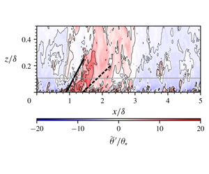
Figure 2. Probability density functions of fluctuating streamwise velocity  $\widetilde{u}((x),t)/u_{\unicode[STIX]{x1D70F}}$ at
  $z/\unicode[STIX]{x1D6FF}=0.05$ (a,c,e,g,i,k) and conditionally averaged streamwise velocity field (b,d,f,h,j,l)
  $\widetilde{u}^{\prime }(\boldsymbol{x})/u_{\unicode[STIX]{x1D70F}}$ (2.2) from LES, for stability parameters noted in the legend. Conditional sampling thresholds
  $\unicode[STIX]{x1D6FC}^{-}=-2\unicode[STIX]{x1D70E}_{\widetilde{u}^{\prime }(\boldsymbol{x}_{c},t)/u_{\unicode[STIX]{x1D70F}}}$ are denoted by the vertical dashed line in (a,c,e,g,i,k). (b,d,f,h,j,l) Streamwise velocity field from LES, conditionally averaged on low-momentum regions
  $\hat{\tilde{u} }^{\prime }(\boldsymbol{x},t)=\langle \widetilde{u}^{\prime }(\boldsymbol{x},t)/u_{\unicode[STIX]{x1D70F}}|\widetilde{u}^{\prime }(\boldsymbol{x}_{c},t)/u_{\unicode[STIX]{x1D70F}}<-2\unicode[STIX]{x1D70E}_{\widetilde{u}^{\prime }(\boldsymbol{x}_{c})/u_{\unicode[STIX]{x1D70F}}}\rangle$, where
  $\boldsymbol{x}_{c}=\{x,y,0.05\unicode[STIX]{x1D6FF}\}$ is the location of the detection criterion (denoted by the horizontal grey line in the velocity field plots). (a,b)
  $-\unicode[STIX]{x1D701}_{\unicode[STIX]{x1D6FF}}=0.31$, (c,d)
  $-\unicode[STIX]{x1D701}_{\unicode[STIX]{x1D6FF}}=1.81$, (e,f)
  $-\unicode[STIX]{x1D701}_{\unicode[STIX]{x1D6FF}}=4.54$, (g,h)
  $-\unicode[STIX]{x1D701}_{\unicode[STIX]{x1D6FF}}=9.38$, (i,j)
  $-\unicode[STIX]{x1D701}_{\unicode[STIX]{x1D6FF}}=27.9$ and (k,l)
  $-\unicode[STIX]{x1D701}_{\unicode[STIX]{x1D6FF}}=266.5$. Solid black lines indicate inclination angles
  $\unicode[STIX]{x1D6FE}(\unicode[STIX]{x1D701}_{z})$ calculated from (3.2) and dashed black lines indicate the angle of the wedge substructure
  $\unicode[STIX]{x1D6FE}_{w}(\unicode[STIX]{x1D701}_{z})=\unicode[STIX]{x1D6FE}(\unicode[STIX]{x1D701}_{z})-\unicode[STIX]{x1D6FE}_{0}$.
Figure 2(a,c,e,g,i,k) shows probability density functions (PDFs) of fluctuating streamwise velocity,  $\tilde{u} ^{\prime }(\boldsymbol{x},t)=\tilde{u} (\boldsymbol{x},t)-\langle \tilde{u} (\boldsymbol{x},t)\rangle _{xyt}$, where there exists Reynolds- and plane-averaged equivalence under the presumed existence of horizontal statistical homogeneity. Values of the global stability parameter
  $-\unicode[STIX]{x1D701}_{\unicode[STIX]{x1D6FF}}$ increase from top to bottom (see table 1 for simulation details). The PDFs show thresholds,
  $\unicode[STIX]{x1D6FC}^{-}=-2\unicode[STIX]{x1D70E}_{\widetilde{u}^{\prime }(\boldsymbol{x}_{c},t)/u_{\unicode[STIX]{x1D70F}}}$, which are used when conditionally sampling LMRs from LES output. Figure 2(b,d,f,h,j,l) shows the corresponding conditionally sampled streamwise velocity:
 $$\begin{eqnarray}{\displaystyle \frac{\hat{\tilde{u} }^{\prime }(\boldsymbol{x},t)}{u_{\unicode[STIX]{x1D70F}}}}=\left\langle \left.{\displaystyle \frac{\widetilde{u}^{\prime }(\boldsymbol{x},t)}{u_{\unicode[STIX]{x1D70F}}}}\right|{\displaystyle \frac{\widetilde{u}^{\prime }(\boldsymbol{x}_{c},t)}{u_{\unicode[STIX]{x1D70F}}}}<-2{\displaystyle \frac{\unicode[STIX]{x1D70E}_{\widetilde{u}^{\prime }(\boldsymbol{x}_{c})}}{u_{\unicode[STIX]{x1D70F}}}}\right\rangle _{N_{\unicode[STIX]{x1D6FC}^{-}}},\end{eqnarray}$$
 where  $\boldsymbol{x}_{c}=\{x,y,0.05\unicode[STIX]{x1D6FF}\}$ is the location of the detection criterion and
  $N_{\unicode[STIX]{x1D6FC}^{-}}$ is the integer number of
  $\widetilde{u}^{\prime }(\boldsymbol{x}_{c},t)/u_{\unicode[STIX]{x1D70F}}<-2\unicode[STIX]{x1D70E}_{\widetilde{u}^{\prime }(\boldsymbol{x}_{c})}/u_{\unicode[STIX]{x1D70F}}$ realizations (for example, Antonia Reference Antonia1981). Superimposed upon the
  $\hat{\tilde{u} }^{\prime }(\boldsymbol{x},t)$ colour floods are inclination angles,
  $\unicode[STIX]{x1D6FE}(\unicode[STIX]{x1D701}_{z})$ (solid black, equation (2.1)) and
  $\unicode[STIX]{x1D6FE}_{w}(\unicode[STIX]{x1D701}_{z})$. The colour flood contours show clear steepening of the conditionally sampled LMRs for increasingly unstable conditions, which previously has been interpreted as a ‘structural thickening’ (sketched on the figure 3a schematic; see also Salesky & Anderson Reference Salesky and Anderson2018). However, the present analysis based upon instantaneous flow visualization (figure 1) and conditional sampling (figure 2) offers compelling evidence that the perceived ‘inclination’ is actually a product of the lower wedge (sketched on the figure 3b schematic, which shows the ostensible ‘lift up’ of the downstream edge of thermally forced LMRs). Results of sampling based upon other quantities are not shown, for brevity, since the resultant scientific deductions are equivalent. Figure 3(c) illustrates the inclined LMR, due to the existence of a lower wedge, in agreement with the smoke visualization results provided by Hommema & Adrian (Reference Hommema and Adrian2003) (a theoretical approach for predicting the wedge angle, and thus overall inclination, follows in § 3).

Figure 3. Schematic illustrating conceptual interpretation of LSM thickening (a), contrasted against results presented in Hommema & Adrian (Reference Hommema and Adrian2003) and herein (b,c), wherein LSMs remain notionally self-similar (b) but are inclined due to formation of a lower wedge (c). Here  $\unicode[STIX]{x1D6FE}(\unicode[STIX]{x1D701}_{z})$ is the stability-dependent inclination angle,
  $\unicode[STIX]{x1D6FE}_{0}=12^{\circ }{-}15^{\circ }$ is the observed inclination angle for neutrally stratified conditions, and
  $\unicode[STIX]{x1D6FE}_{w}(\unicode[STIX]{x1D701}_{z})$ is the angle of the wedge substructure.
3 Theory
Beginning with arguments set forth in Hommema & Adrian (Reference Hommema and Adrian2003), one can derive a prognostic closure for the inclination angle of LSMs for increasingly unstable thermal stratification, as characterized by the Monin–Obukhov stability parameter  $\unicode[STIX]{x1D701}_{z}$. The inclination angle
  $\unicode[STIX]{x1D6FE}$ of an LSM can be written as
  $\unicode[STIX]{x1D6FE}\approx (w/u)$, where
  $u$ and
  $w$ are, respectively, the characteristic streamwise and vertical velocity components within an LSM used in this section to denote velocity components). In an unstably stratified flow over a solid boundary, the vertical velocity component can be written as
  $w=w_{p}+w_{\unicode[STIX]{x1D703}}$, where
  $w_{p}$ is the vertical velocity due to packet motion and
  $w_{\unicode[STIX]{x1D703}}$ is vertical velocity due to buoyancy. The inclination angle can then be written as
 $$\begin{eqnarray}\unicode[STIX]{x1D6FE}=\tan ^{-1}\left[\frac{w_{p}}{u}+\frac{w_{\unicode[STIX]{x1D703}}}{u}\right].\end{eqnarray}$$
 In the absence of buoyancy ( $w_{\unicode[STIX]{x1D703}}=0$), one should recover the inclination angle
  $\unicode[STIX]{x1D6FE}_{0}=12^{\circ }{-}15^{\circ }$ observed for neutrally stratified conditions (Carper & Porté-Agel Reference Carper and Porté-Agel2004; Marusic & Heuer Reference Marusic and Heuer2007), which implies that
  $w_{p}/u=\tan \unicode[STIX]{x1D6FE}_{0}$. The characteristic streamwise velocity scale can be expressed in terms of the friction velocity,
  $u=u_{\unicode[STIX]{x1D70F}}$; the vertical velocity due to buoyancy can be expressed in terms of the free convective velocity scale
  $u_{f}$ (Wyngaard Reference Wyngaard2010) – that is,
  $w_{\unicode[STIX]{x1D703}}=c_{1}u_{f}=c_{1}(gzQ_{0}/\unicode[STIX]{x1D6E9}_{0})^{1/3}$, where
  $c_{1}$ is a constant (to be determined empirically). Equation (3.1) can then be written as
 $$\begin{eqnarray}\displaystyle \unicode[STIX]{x1D6FE}(\unicode[STIX]{x1D701}_{z}) & = & \displaystyle \tan ^{-1}[\tan \unicode[STIX]{x1D6FE}_{0}+c_{1}\unicode[STIX]{x1D705}^{-1/3}(-\unicode[STIX]{x1D701}_{z})^{1/3}]\end{eqnarray}$$
 $$\begin{eqnarray}\displaystyle & {\approx} & \displaystyle \unicode[STIX]{x1D6FE}_{0}+\underbrace{\tan ^{-1}[c_{2}\unicode[STIX]{x1D705}^{-1/3}(-\unicode[STIX]{x1D701}_{z})^{1/3}]}_{\unicode[STIX]{x1D6FE}_{w}(\unicode[STIX]{x1D701}_{z})},\end{eqnarray}$$
 where (3.2) is exact, and (3.3), obtained using the small-angle approximation, allows one to interpret structure inclination angle  $\unicode[STIX]{x1D6FE}(\unicode[STIX]{x1D701}_{z})$ as the sum of the angle for neutral conditions
  $\unicode[STIX]{x1D6FE}_{0}$ and the stability-dependent inclination of the high-momentum wedge
  $\unicode[STIX]{x1D6FE}_{w}(\unicode[STIX]{x1D701}_{z})$. Fitting (3.2) and (3.3) to inclination angles calculated from
  $R_{uu}$ from the AHATS dataset (discussed in § 4) with
  $\unicode[STIX]{x1D6FE}_{0}=12^{\circ }$ yields empirical values of
  $c_{1}=0.569$ and
  $c_{2}=0.492$. The approximate equation for
  $\unicode[STIX]{x1D6FE}(\unicode[STIX]{x1D701}_{z})$ (3.3) is within
  ${\sim}1^{\circ }$ of the exact expression (3.2) for
  $-\unicode[STIX]{x1D701}_{z}\leqslant 1$ and within
  ${\sim}5^{\circ }$ for
  $-\unicode[STIX]{x1D701}_{z}=10$.
4 Literature data

Figure 4. Structure inclination angles  $\unicode[STIX]{x1D6FE}$ (left ordinate) and corresponding wedge inclination angles
  $\unicode[STIX]{x1D6FE}_{w}$ (right ordinate, calculated assuming
  $\unicode[STIX]{x1D6FE}_{0}=12^{\circ }$) as a function of the MO stability variable
  $-\unicode[STIX]{x1D701}_{z}$ calculated from the AHATS data and LES for unstable thermal stratification. Data points are also displayed from the unstable atmospheric surface layer observations of Carper & Porté-Agel (Reference Carper and Porté-Agel2004), Chauhan et al. (Reference Chauhan, Hutchins, Monty and Marusic2013) and Marusic & Heuer (Reference Marusic and Heuer2007), as well as the LES of Salesky & Anderson (Reference Salesky and Anderson2018). The empirical fit from Chauhan et al. (Reference Chauhan, Hutchins, Monty and Marusic2013) (4.1) is shown for comparison; the prediction of the prognostic closure (3.2) is denoted by the solid black lines, plotted for
  $\unicode[STIX]{x1D6FE}_{0}=12^{\circ }$,
  $15^{\circ }$,
  $18^{\circ }$. The shaded grey region indicates the range of inclination angles (
 $\unicode[STIX]{x1D6FE}_{0}$, corresponding to the left ordinate) observed for neutral stratification (for example, Hommema & Adrian Reference Hommema and Adrian2003, figure 11(a)).
Structure inclination angles  $\unicode[STIX]{x1D6FE}$ as a function of the stability variable
  $-\unicode[STIX]{x1D701}_{z}$ are displayed in figure 4 based on published studies using atmospheric surface layer observations (Carper & Porté-Agel Reference Carper and Porté-Agel2004; Marusic & Heuer Reference Marusic and Heuer2007; Chauhan et al. Reference Chauhan, Hutchins, Monty and Marusic2013), previous LES results (Salesky & Anderson Reference Salesky and Anderson2018), the suite of LES runs detailed in table 1, and additional atmospheric surface layer observations from the advection horizontal array turbulence study (AHATS) dataset. The observational studies by Carper & Porté-Agel (Reference Carper and Porté-Agel2004), Marusic & Heuer (Reference Marusic and Heuer2007) and Chauhan et al. (Reference Chauhan, Hutchins, Monty and Marusic2013) were all conducted at the SLTEST facility on the salt flats of western Utah; structure inclination angles in each study were calculated following the procedure described in § 2, where the two-point correlation of streamwise velocity
  $R_{uu}(\unicode[STIX]{x0394}x,\unicode[STIX]{x0394}z;\unicode[STIX]{x1D701}_{z})$ (2.1) was calculated, and the inclination angle was calculated via
  $\unicode[STIX]{x1D6FE}=\tan ^{-1}(\langle \unicode[STIX]{x0394}z/\unicode[STIX]{x0394}x^{\star }\rangle )$. In each case, the stability variable
  $-\unicode[STIX]{x1D701}_{z}$ used for plotting
  $\unicode[STIX]{x1D6FE}(\unicode[STIX]{x1D701}_{z})$ is taken from the reference location (that is, the lowest height used in the calculation of
  $R_{uu}(\unicode[STIX]{x0394}x,\unicode[STIX]{x0394}z)$), consistent with previous studies (Chauhan et al. Reference Chauhan, Hutchins, Monty and Marusic2013). While structure inclination angle is a function of
  $z$ in the general case, the observational data only allow us to calculate
  $\unicode[STIX]{x1D6FE}$ for structures in close proximity to the wall.
The AHATS dataset was collected from 25 June to 16 August, 2008 near Kettleman City, CA, USA. The surrounding terrain was predominantly level and horizontally homogeneous. We used data from the AHATS profile tower, consisting of Campbell Scientific CSAT-3 sonic anemometers at  $z=1.51$, 3.30, 4.24, 5.53, 7.08 and 8.05 m, which sampled the wind velocity vector (
 $u,v,w$) and sonic temperature
  $\unicode[STIX]{x1D703}$ at 60 Hz. The raw 60 Hz data were downsampled to 20 Hz and analysed in 27.3 min blocks, corresponding to 32 768 data points. Only runs with mean wind angles within
  $\pm 45^{\circ }$ of the anemometer axis were included in the analysis, in order to minimize the influence of flow distortion. A coordinate rotation of the raw anemometer data was employed so that the coordinate system was aligned with the mean wind direction (i.e.
  $\langle v\rangle _{t}=0$); standard data quality control criteria were employed to exclude non-stationary blocks from the data analysis (discussed further in Salesky & Chamecki (Reference Salesky and Chamecki2012)).
Figure 4 illustrates that the proposed model for LSM inclination angle (3.2), plotted for several values of  $\unicode[STIX]{x1D6FE}_{0}$ (with
  $c_{1}=0.569$), is in good agreement with both LES results and field observations across the range of stabilities (
 $-\unicode[STIX]{x1D701}_{z}\in [10^{-3},10^{1}]$) captured by the various datasets. The range of inclination angles
  $\unicode[STIX]{x1D6FE}_{0}$ reported for neutrally stratified conditions (see, for example, figure 11(a) of Hommema & Adrian (Reference Hommema and Adrian2003)) is denoted in figure 4 by the grey shaded region. Note that, even in the neutrally stratified case, significant variability has been observed around the typically cited value of
  $\unicode[STIX]{x1D6FE}_{0}=12^{\circ }{-}15^{\circ }$. Also displayed in figure 4 is the empirical fit proposed by Chauhan et al. (Reference Chauhan, Hutchins, Monty and Marusic2013):
 $$\begin{eqnarray}\unicode[STIX]{x1D6FE}(\unicode[STIX]{x1D701}_{z})=12.0+7.3\ln (1-70\unicode[STIX]{x1D701}_{z}).\end{eqnarray}$$
While both curves capture the observed increase in LSM inclination angles, we note that (4.1) is an empirical fit to the data. Equation (3.2) is based on the theory presented in § 3, and captures the observed behaviour of the downstream edge of an LSM lifting up from the wall with the formation of a high-momentum wedge beneath.
5 Conclusions
Observations and numerical simulations of unstably stratified, high- $Re_{\unicode[STIX]{x1D70F}}$, channel turbulence have demonstrated that the inclination angle
  $\unicode[STIX]{x1D6FE}$ of large-scale motions increases systematically with increasing buoyancy forcing (Hommema & Adrian Reference Hommema and Adrian2003; Carper & Porté-Agel Reference Carper and Porté-Agel2004; Marusic & Heuer Reference Marusic and Heuer2007; Chauhan et al. Reference Chauhan, Hutchins, Monty and Marusic2013; Salesky & Anderson Reference Salesky and Anderson2018) beyond the value
  $\unicode[STIX]{x1D6FE}_{0}=12^{\circ }{-}15^{\circ }$ observed for neutral conditions. However, the effects of unstable thermal stratification on the morphological properties of LSMs, and the connections between LSM structure and observed inclination angles, are not well understood. Some authors have proposed that LSMs incline and thicken while remaining attached to the wall (Salesky & Anderson Reference Salesky and Anderson2018), while others have suggested that the downstream edge of an LSM lifts away from the wall (Hommema & Adrian Reference Hommema and Adrian2003) as buoyancy forcing increases.
Using a suite of LES of turbulent channel flow spanning a range of unstable thermal stratification conditions, we use instantaneous flow visualizations and conditional sampling to demonstrate that buoyancy causes the downstream edge of an LSM to lift away from the wall, leaving a wedge of high-momentum fluid beneath, in agreement with the smoke visualizations of Hommema & Adrian (Reference Hommema and Adrian2003). A new prognostic model is developed for LSM inclination angle that accounts for this observed structure; we demonstrate that the inclination angle  $\unicode[STIX]{x1D6FE}$ of an LSM can be expressed as the sum of the neutral inclination angle
  $\unicode[STIX]{x1D6FE}_{0}\approx 12^{\circ }$ and the stability-dependent inclination angle of the high-momentum wedge
  $\unicode[STIX]{x1D6FE}_{w}(\unicode[STIX]{x1D701}_{z})$. Available data from the literature, atmospheric surface layer observations from the AHATS and SLTEST experiments, as well as the LES presented herein, are found to be in good agreement with the prognostic model.
Table 1. Properties of LES cases: mean pressure gradient force,  $-\unicode[STIX]{x1D70C}_{0}^{-1}(\text{d}P/\text{d}x)$; kinematic surface heat flux,
  $Q_{0}$; flow depth,
  $\unicode[STIX]{x1D6FF}$; Obukhov length,
  $L$; global stability parameter,
  $\unicode[STIX]{x1D701}_{\unicode[STIX]{x1D6FF}}=-\unicode[STIX]{x1D6FF}/L$; friction velocity,
  $u_{\unicode[STIX]{x1D70F}}$; and Deardorff convective velocity scale,
  $w_{\star }$.

Acknowledgement
This work was supported by the National Science Foundation, grant no. AGS-1500224 (WA).
Declaration of interests
The authors report no conflict of interest.
Appendix. Large-eddy simulation: numerical procedure, cases
A suite of six LES cases were run in a similar configuration to the LES described in Salesky & Anderson (Reference Salesky and Anderson2018). The simulations were configured to replicate a convective atmospheric boundary layer; the initial condition for the temperature field includes a capping inversion, where the boundary layer depth  $\unicode[STIX]{x1D6FF}$ corresponds to the height at which the total heat flux
  $\langle \widetilde{w}^{\prime }\widetilde{\unicode[STIX]{x1D703}}^{\prime }\rangle +\langle q_{3}^{sgs}\rangle$ attains its most negative value (Salesky & Anderson Reference Salesky and Anderson2018). The domain size was set to
  $\{L_{x}/\unicode[STIX]{x1D6FF}_{0},L_{y}/\unicode[STIX]{x1D6FF}_{0},L_{z}/\unicode[STIX]{x1D6FF}_{0}\}=\{6,6,2\}$ (where
  $\unicode[STIX]{x1D6FF}_{0}=1000~\text{m}$ is the initial boundary layer depth), with a grid resolution of
  $N_{x}N_{y}N_{z}=256^{3}$, corresponding to an LES filter width of
  $\unicode[STIX]{x1D6E5}_{x}/\unicode[STIX]{x1D6FF}=\unicode[STIX]{x1D6E5}_{y}/\unicode[STIX]{x1D6FF}\approx 2.3\times 10^{-2}$ and
  $\unicode[STIX]{x1D6E5}_{z}/\unicode[STIX]{x1D6FF}\approx 7.8\times 10^{-2}$. The computational domain is sufficient to resolve LSMs for all table 1 cases (Salesky & Anderson Reference Salesky and Anderson2018), but not VLSMs. However, since VLSMs form via quasi-streamwise coalescence of LSMs, omission of LSMs does not undermine the generality of this article (Hutchins & Marusic Reference Hutchins and Marusic2007); rather, it is preferable to allocate greater spatial resolution to LSMs. The time step was set to
  $\unicode[STIX]{x1D6E5}_{t}=0.03~\text{s}$. Simulations were run for a total of 480 000 steps, which corresponds to
  ${\sim}17.7$ convective turnover times (
 $T_{\ell }=\unicode[STIX]{x1D6FF}/w_{\star }$) for the least convective (
 $-\unicode[STIX]{x1D6FF}/L=0.31$) case (where
  $T_{\ell }=27\,000\unicode[STIX]{x1D6E5}_{t}$) and
  ${\sim}26.0T_{\ell }$ for the most convective (
 $-\unicode[STIX]{x1D6FF}/L$) case (where
  $T_{\ell }=18\,500\unicode[STIX]{x1D6E5}_{t}$). Simulations were forced by a mean horizontal pressure gradient force
  $-(1/\unicode[STIX]{x1D70C}_{0})(\text{d}P/\text{d}x)$ with a constant surface heat flux
  $Q_{0}$ (values of forcing parameters can be found in table 1). In contrast to the LES results presented in Salesky & Anderson (Reference Salesky and Anderson2018), the present simulations were run without Coriolis in order to ensure that LSMs were aligned with the
  $x$-coordinate axis at all heights for flow visualization purposes. All other initial and boundary conditions are identical to those presented in Salesky & Anderson (Reference Salesky and Anderson2018). Note that the present simulations have higher spatial resolution than the highest-resolution cases presented in Salesky & Anderson (Reference Salesky and Anderson2018); thus sensitivity to the numerical grid employed is expected to be minimal (grid invariance has been previously established and presented in the appendix of Salesky et al. (Reference Salesky, Chamecki and Bou-Zeid2017)). The forcing used for each simulation, boundary layer depth
  $\unicode[STIX]{x1D6FF}$, Obukhov length
  $L$, friction velocity
  $u_{\unicode[STIX]{x1D70F}}$, bulk stability parameter
  $\unicode[STIX]{x1D701}_{\unicode[STIX]{x1D6FF}}=-\unicode[STIX]{x1D6FF}/L$, and Deardorff convective velocity scale
  $w_{\star }=(g\unicode[STIX]{x1D6FF}Q_{0}/\unicode[STIX]{x1D6E9}_{0})^{1/3}$ (where
  $g$ is gravity and
  $\unicode[STIX]{x1D6E9}_{0}$ is a reference potential temperature at the surface) can be found in table 1.


