1. INTRODUCTION
Over the last decade, Differential Global Positioning Systems (DGPS) have become a standard method to improve the positioning performance of the user receivers in a wide range of GPS applications. In a standard DGPS operation, the reference station calculates differential corrections that are transmitted to user receivers that are used to eliminate satellite clock error and to mitigate the other correlated errors due to orbit, troposphere and ionosphere. Nevertheless, the effectiveness of the differential corrections is influenced by spatial and temporal variations of these correlated errors. This effect is also known as DGPS error growth which degrades the DGPS accuracy at the user site. Since the removal of Selective Availability (SA) in 2000, the temporal decorrelation of DGPS errors have become insignificant and resulted in more reliable DGPS corrections over a long period (Park et al., Reference Park, Kim and Kee.2006). However, DGPS users are still challenged by the great accuracy degradation arising from the decorrelation of these errors in a spatial sense, i.e., as the separation distance increases between reference and user station.
A few studies have been conducted on DGPS error growth over distance. Monteiro et al. (Reference Monteiro, Moore and Hill2005) and Misra and Enge (Reference Misra and Enge2004) found that for a separation of reference and user station of 100 km, the spatial effect of orbital and tropospheric errors is less than 0·01 m and 0·1 m, respectively. They also found that the orbital and tropospheric errors change slowly over tens of minutes and can be removed almost entirely by the differential corrections. On the other hand, the ionospheric error is found to have the largest effect that decorrelates the differential corrections between reference and user stations and thus degrades the DGPS positioning results (Park et al., Reference Park, Kim and Kee.2006). Such scenarios are worse in the equatorial area and the ionospheric effects are much less understood than in other regions (Schunk and Nagy, Reference Schunk and Nagy2000).
DGPS error growth over the Malaysian sector is fairly unquantified due to insufficient research with very few resources deployed to investigate the ionospheric effects on DGPS corrections. This paper investigates the Equatorial ionosphere and its effects on DGPS error growth over Malaysia by using a network of GPS Continuously Operating Reference Station (CORS). The analysis has been conducted during the seasons of the two equinoxes and solstices that demonstrate significant ionospheric variations in Malaysia. In addition, a regression model of the ionospheric errors has been developed and further analysis was conducted to validate this model with the observed ionospheric errors during the maximum solar year of 2013 by using internet-based DGPS. Finally, some conclusions were drawn to summarise this study.
2. IONOSPHERIC ERROR IN DGPS CORRECTIONS
The ionosphere is part of the Earth's atmosphere where solar radiation is predominantly active due to ultra-violet radiation as a result of ionisation. The ionosphere layer starts from about 50 km and extends over a thousand kilometres or so in height above the Earth's surface. The Total Electron Content (TEC), which is the total number of electrons present along a trans-ionospheric radio signal path between two points, is often used to quantify the ionosphere of the Earth (Klobuchar, Reference Klobuchar1991, Reference Klobuchar, Parkinson, Spilker, Axelrad and Enge1996; Langley Reference Langley2000). The TEC is highly variable, in both a spatial and temporal sense, and the magnitude varies based on the season and the time of day. However, the major factors are the level of solar activity and the geomagnetic location on the Earth. Figure 1 indicates that the Equatorial region is the area that experiences a high magnitude of TEC. This natural phenomenon of the Equatorial ionosphere has attracted the attention of many scientists studying space weather (Musa et al., Reference Musa, Lim, Yan and Rizos2006), nevertheless, it is still a challenge for satellite-based positioning applications (Chen et al., Reference Chen, Gao, Hu, Chen and Ding2007).

Figure 1. Global TEC Map (http://www.ips.gov.au/Satellite/2/1/5).
As GPS radio signals propagate through the Earth's ionosphere, the transmission of the signals is delayed. A change in signal speed changes the signal transit time and consequently the ‘measured’ range between the satellite and the receiver is different from its ‘line-of-sight’ geometric range. This range difference due to the effect of the ionospheric delay can be measured with GPS multi-frequencies and mapped in zenith direction using Equation (1); where I z is the ionospheric zenith delay (i.e., VTEC) expressed in units of length; f is the frequency of the L1 signal; φ is the satellite elevation angle at the ionosphere pierce point; and the TEC along the path of the signal (Hofmann-Wellenhof et al., Reference Hofmann-Wellenhof, Lichtenegger and Collins1992);
 $$I_Z = \displaystyle{1 \over {\sin \!\phi}} \displaystyle{{40 {\cdot} 3} \over f}TEC $$
In DGPS correction generation at reference station r (as in Equation (2)), ionospheric error, other correlated errors, satellite and reference station receiver dependent errors are estimated in the form of Pseudorange Correction (PRC) for every satellite S at reference epoch (t). The code pseudorange as measured by user station u (as in Equation (3)), will apply the DGPS correction to correct its measurement and yield corrected pseudorange, which can be expressed as in Equation (4).
 $${\rm PRC}^S (t) = - I_{z,r}^S (t) - \varepsilon_r^S (t) - p_r (t) + p^S (t) $$
 $$R_u^S (t) = \ell_u^S (t) + I_{z,u}^S (t) + \varepsilon _u^S - p^S (t) + p_u (t)$$
 $$R_{u \, corr}^S (t) = R_u^S (t) + {\rm PRC}^S (t)$$
where (t) is the reference epoch, PRCS are DGPS corrections (Pseudorange Correction of Satellite S), R uS is the code pseudorange correction of satellite S as measured by the user station and R u corrS is the corrected code pseudorange at the user station.  $\ell _u^S $ is the geometric range from the satellite S to the user station, I z,rS is the ionospheric zenith delay at the reference station and I z,uS is the ionospheric zenith delay at the user station. ε rS and ε uS are other correlated errors (such as orbital and tropospheric delay), pS is satellite dependant error (such as clock and hardware errors), p r is receiver dependent errors at the reference station and p u is user dependent error at the reference station.
Substituting Equations (2) and (3) into Equation (4) yields;
 $$R_{u \, corr}^S (t) = \ell _u^S (t) + [\Delta I_{z,ur}^S (t) + \Delta \varepsilon _{ur}^S (t) + \Delta \rho_{ur} (t)]$$
where ΔI z,urS is the differential between ionospheric zenith delay at user and reference station, Δε urS is the differential between correlated errors (orbital and tropospheric error) at the user and reference stations and Δ ρ ur is the differential between the station dependent errors at the user and reference stations.
The corrected range in Equation (5) will be used in the calculation of the user's differential position (X u, Yu, Zu) with respect to the satellite position (see Equation 6).
 $$R_{u}^S (t)_{corr} \equiv f\,(X_u, Y_u, Z_u )$$
The non-linear equation can be solved by applying linearization equation (Grafarend and Shan, Reference Grafarend and Shan2002). It is noted that the accuracy of the user differentially corrected position relies on the effectiveness of user corrected pseudoranges to exploit all the errors in Equation (5). Nevertheless, the remaining error will be propagated into the user position in Equation (6).
For users near a reference station, the respective signal paths from the satellite are sufficiently close so that the differential of ionospheric error or ΔI z,urS is almost eliminated. However, once the distance from the user to the reference station increases, the ionosphere may be different at both stations and cause different delays. The decorrelation of this ionospheric error can be influenced by the incidence angle (i.e., the elevation angles at the ionospheric pierce point) of GPS signals and density of TEC at both stations. Monteiro et al. (Reference Monteiro, Moore and Hill2005) found that the delays experienced by the reference station and the user at 100 km apart due to the elevation angle are typically 0·03 m, but can be greater than 4 m over 100 km when the ionosphere is disturbed.
3. MALAYSIA GPS CORS DATA AND METHODOLOGY
The DGPS error growth due to ionospheric effects is studied by analysing the GPS dual-frequency data from two GPS networks in Malaysia, i.e., MyRTKnet and ISKANDARnet (see Figure 2). Currently, the MyRTKnet consists of 50 CORS in Peninsular Malaysia and 28 CORS in East Malaysia, which is operated by the Department of Survey and Mapping Malaysia (DSMM) to support surveying and geodetic activities. Meanwhile, the ISKANDARnet consists of four CORS located at the southern part of Peninsular Malaysia which is managed by the GNSS and Geodynamics Research Group at Universiti Teknologi Malaysia (UTM) for research and academic activities. In addition to these networks, another six GPS stations of the International Global Navigation Satellite System (GNSS) Service (IGS) have been utilised in this study that covers approximately 15°S to 15°N in latitude and 95°E to 130°E in longitude.

Figure 2. Location of GPS stations for MyRTKnet and ISK1 station of ISKANDARnet (left), and IGS (right).
One year of continuous GPS data in 2010 has been post-processed using the Precise Point Positioning (PPP) approach with Bernese 5·0 software (Dach et al., Reference Dach, Hugentobler, Fridez and Meindl2007). Processing strategies and model parameters are depicted in Table 1. The geometry-free (L4) linear combination which contains ionospheric information in the TEC Units (TECU) was analysed. Following Schaer (Reference Schaer1999), the TEC was developed into a series of spherical harmonics adopting a single-layer model set at an altitude of 450 km in a sun-fixed reference frame. The sun-fixed reference frame allows creation of a “frozen ionosphere” model that refers to the specific time intervals presenting the state of the ionosphere over the region usually for a 24-hour period in one map (Wielgosz et al., Reference Wielgosz, Grejner-Brzezinska and Kashani2003). Slant TEC values along oblique GPS signal paths were quantified from the ISKANDARnet1 (ISK1), MyRTKnet and IGS stations which were then converted to vertical TEC by means of the single layer mapping function. The variation of ionospheric delay was mapped in the zenith direction using Equation (1). These results were analysed in four seasons; winter-solstice (22 December – 19 March), vernal-equinox (20 March – 21 Jun), summer-solstice (22 Jun – 21 September), and autumnal-equinox (22 September – 21 December).
Table 1. Processing parameters and strategy to derive ionospheric zenith delay using GPS network.

The DGPS error growth was evaluated based on user positional error at different locations of user stations over Malaysia. In this experiment, ISK1 was treated as the reference station while the other 78 MyRTKnet stations were treated as user stations. This arrangement is meant to provide sufficient information on the DGPS error growth according to the ionosphere gradient that usually occurs in the latitudinal direction. The PRC was generated from ISK1 in post-processing mode by using pseudorange measurement from the L1 frequency which follows Equations (2) – (6). During the processing, elevation mask angles at the user stations were set to 10° so as to minimise the remaining noise due to low elevation satellites. The users' DGPS positional error at all user stations were calculated by;
 $$(\Delta X_u, \Delta\! Y_u, \Delta Z_u ) = (X_u^{\prime}, Y_u^{\prime}, Z_u^{\prime} ) - (X_u, Y_u, Z_u )$$
where (X′ u, Y′u, Z′u) is the most probable (‘known’) coordinate of the user stations which was previously determined from precise carrier-phase GPS static processing technique. Finally, the DGPS positional error growth according to distance between ISK1 and user stations were categorised into four seasons as mentioned above.
4. RESULTS AND DISCUSSION
4.1. Ionosphere trend in Malaysia
The resulting seasonal ionospheric zenith delay map is shown in Figure 3. Table 2 summarises the maximum and minimum average of the ionospheric zenith delay, as well as the rate of change of the delay in latitudinal and longitudinal directions.

Figure 3. Seasonally ionospheric zenith delay map representing winter-solstice, vernal-equinox, summer-solstice and autumnal-equinox, respectively.
Table 2. The statistics of ionospheric zenith delay in 2010 according to Figure 3.

Table 3. Linear trends of seasonal DGPS positional errors (S is the distance between user and reference station, E is an exponential [×10]).

The ionospheric zenith delay within this region lies in the range 2 m – 2·653 m during the two solstices and 2·451 m – 3·344 m during the two equinoxes. The highest minimum and maximum values of the delay can be found during the two equinoxes. The highest is during the autumnal-equinox with maximum delay reaching up to 3·344 m and its rate of change at 9·8 and 0·3 in the latitudinal and longitudinal directions, respectively. Meanwhile, the lowest delay was found during the winter-solstice but has a high rate of change of 6·2 in latitudinal direction in comparison to the vernal-equinox and summer-solstice. Figure 3 also shows obvious trends of the delay during the four seasons - it increases significantly with decreasing latitude, which is in agreement with the initial equatorial TEC investigation by Musa et al., (Reference Musa, Leong, Abdullah and Othman2012).
This scenario is explained by the geographical location of Malaysia that sits under the southern crest of Equatorial Ionization Anomaly (EIA) and near to the magnetic dip equator where the magnetic field is horizontal. The EIA is attributed to the so-called equatorial plasma that are being lifted by the eastward electric field, and thereafter diffuse down along the magnetic field line to higher latitudes under the influence of gravitational force. The formation of EIA is also recognised as a “fountain effect” creating two plasma peaks on either side of the magnetic equator at approximately 15° geomagnetic latitudes.
4.2. DGPS Error Growth in Malaysia
Figure 4 shows the mean Root Mean Square (RMS) of position errors for all user stations over four seasons. These values show an increment that is proportional to the distance of the user station from the reference, ISK1, i.e., it is distance dependent. Furthermore, the DGPS error growth demonstrates remarkable seasonal variations similar to ionospheric zenith delay as discussed in Section 4.1. It also can be seen that the user positional errors during vernal and autumnal equinoxes are generally higher than the other seasons of summer and winter solstices, which is further explained in Figure 5.

Figure 4. DGPS accuracy from ISK1.

Figure 5. DGPS positional error (estimated position DGPS – ‘known’) growth with distance at different seasons, E is an exponential [×10]).
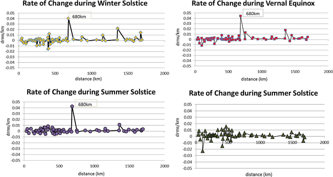
From Figure 5, the mean intercept for all regression lines is 0·203 m, which represents the minimum DGPS positional errors. During the seasons of highest ionospheric errors, multipliers in their linear function as in Table 3 are 1·6 mm/km and 1·5 mm/km for the season of vernal-equinox and autumnal-equinox respectively. The multipliers of linear function during low ionospheric errors gradient, i.e., for the season of winter-solstice and summer-solstice, were found to be at 1·1 mm/km and 1·2 mm/km respectively. Autumnal-equinox shows the highest degree of R 2 value of 0·991 as compared to the other seasons. This result indicates that the autumnal-equinox experiences strong decorrelation of DGPS positional errors, according to distance, which also reflects the highest rate of change of ionospheric delay during this season as found in Section 4.1. The rate of change of user positional errors that is proportional to the user distance is illustrated in Figure 6. Rapid spatial rate of change in user position for winter solstice, summer solstice and vernal equinox seasons can be seen at a user separation of 680 km. This can be attributed to high decorrelation of orbital and tropospheric errors that resulted in 0·5 m of user positional errors.

Figure 6. Rate of change during all seasons.
This study also attempts to determine an initial distance at which ionospheric error in DGPS positional errors starts to decorrelate over distance. To account for only ionospheric error effect in DGPS positional errors, the regression lines at a distance less than 680 km were plotted in Figure 7. For this range of user distance, summer-solstice, winter-solstice and vernal-equinoxes depict a 2nd order polynomial with turning point at S′ ss = 100 km, S′ ws = 125 km and S′ ve = 100 km respectively. It can be seen that the DGPS positional error grows slowly and the value is almost equal during these three seasons for the distance less than the turning point. However, the autumnal-equinox shows a linear trend from the minimum user distance onwards.

Figure 7. DGPS positional error (estimated positionDGPS - positionknown) growth with distance <680 km at different seasons, E is an exponential [×10]).
These results suggest that in the case of moderate separation between reference and user stations, the amount of ionospheric delay at both stations are highly correlated. Thus, the influences of ionospheric errors were significantly reduced at the user station by the PRC (see Equations (2)-(6)) and consequently the user position has been significantly improved. Meanwhile, medium and long distances experienced high decorrelation of ionospheric error. Thus PRC as estimated by the reference station become less efficient in order to improve the user position.
4.3. Assessment of the Equatorial DGPS Error Growth Model
In this section, a collaborative work between academic, industry and government agencies in Malaysia was established to provide an internet-based DGPS service for the assessment of the regression model as discussed in Section 4.2. For this service, the setup involves five CORS (see Figure 8). ISK2 station was selected as the reference station and ISK1 as the processing centre to transmit the DGPS correction using the Networked Transport of RTCM via Internet Protocol (NTRIP), while the other CORS were treated as the user stations.

Figure 8. The location of Internet-based DGPS reference stations in Peninsular Malaysia.
The assessment was conducted on 2 November 2013, in the season of autumnal-equinox, where a large ionospheric error effect can be expected. In order to correspond with the discussion in Section 4.3 the assessment was classified into two ranges of distance S, i.e., between reference and user station, S < 680 km and S > 680 km (see Table 4). The RTKLIB software (Takasu, Reference Takasu2013) was used to allow for the real-time internet-based DGPS application. By using this software tool, the DGPS correction was streamed from the reference station to the user station via NTRIP communication. The assessment was conducted simultaneously for all stations involved.
Table 4. Summary of the DGPS stations involved in Internet-based DGPS.
The time series in Figures 9 to 11 show the residual coordinates or positional errors (estimated minus ‘known’ coordinates) and its corresponding statistical Tables 5 to 7 for user stations JLKU, JLML and AGLG respectively. For each user station, the RMS of the horizontal distance from the internet-based DGPS and regression model as obtained in Section 4.2 was also listed in these tables. Overall, the range of the residuals for all stations was found to be ±3 m. In addition, the range of residual variations for these stations as given by the standard deviation in each statistical table was in the range of ±0·4 m in both easting and northing components.

Figure 9. Residual positional accuracy at JLKU.

Figure 10. Residual positional accuracy at JLML.
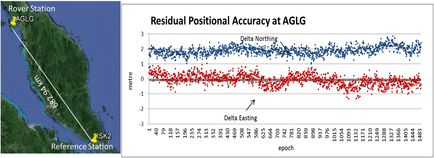
Figure 11. Residual positional accuracy at AGLG.
Table 5. Statistical analysis at JLKU (Distance from ISK2 is 274·13 km).

Table 6. Statistical analysis at JLML (Distance from ISK2 is 526·24 km).

Table 7. Statistical analysis at AGLG (Distance from ISK2 is 682·94 km).

The differences in the RMS of the horizontal distance between the internet-based DGPS and the regression model are depicted in Figure 12. For the user with S < 680 km, the discrepancy of the RMS is within 0·02–0·139 m. Meanwhile, a large discrepancy of about 0·652 m can be seen for S > 680 km. One of the possible reasons for these differences, i.e., between measured and modelled value, could be explained by the fact that the ionospheric error in the year 2013, which is in the year of solar maximum, is greater when compared to the year 2010 when the regression model was derived.

Figure 12. Discrepancies of user RMS from DGPS measurement (2013) and regression model (2010).
5. CONCLUSION
This paper reports spatial and seasonal effects of the equatorial ionospheric errors on DGPS positioning in Malaysia. A local ionospheric map and seasonal ionospheric trends were presented, and a regression model was developed by using the GPS data from the local CORS networks in year 2010. It was found that the spatial variation of ionospheric errors in this region is higher during equinoctial seasons. Findings show that the effect of spatial variation of ionospheric errors in DGPS is very significant when the separation of user and reference station is greater than 680 km. The regression model was tested during the solar maximum year in 2013 by using internet-based DGPS and the results have shown that the model is capable of estimating DGPS positional errors for distances less than 680 km. In future work, a real-time ionospheric modelling service could be developed to support the integrity of DGPS and navigational services in Malaysia.
ACKNOWLEDGMENTS
The authors would like to thank the Department of Survey and Mapping Malaysia (DSMM) and the International GNSS Service (IGS) for providing valuable GPS data. Thanks are also extended to RTKLIB for the open source program package. This research article is funded by research grants of Malaysian Ministry of Science & Technology e-science (4B078), (4B131) and Fundamental Research Grant Projects (4F117).