


Any attempt to study Mesoamerican land surveying starts with the Acolhua codices Vergara (CV) and Santa María Asunción (CSMA). The vast number of agricultural fields (1,589) registered in the codices with detailed information on side lengths and areas provides a unique opportunity for mathematicians interested in the study of ethnomathematics.
This article not only summarizes some of the mathematical results obtained over the years in the study of the Acolhua codices CV and CSMA (see Harvey and Williams Reference Harvey and Williams1980; Jorge et al. Reference Jorge, Williams, Garza-Hume and Olvera2011; Williams and Harvey Reference Williams and Harvey1997; Williams and Hicks Reference Williams and Hicks2011; Williams and Jorge y Jorge Reference Williams and y Jorge2008) but also extends previous results from CV to CSMA and adds some refinements, as we analyze the accuracy of the area computations from both codices. We present for the first time an analysis of polygons with more than four sides from both codices that includes areas and shapes. We look at maximum possible areas and apply the concept of a feasible polygon; considering the possible shapes of polygons with given side lengths and area, we do numerical reconstructions, concluding that the Acolhua were very good surveyors. To guide our research, we created a database that summarizes the information contained in the codices and a computer program that constructs polygons with given side lengths and areas.
This article has three sections: a summary and update of results obtained previously for quadrilaterals in CV, an analysis of the quadrilateral fields of CSMA, and a presentation of the results we have obtained so far for both codices on shapes and areas of the fields with more than four sides. We first present some background information on the Vergara and Santa María Asunción codices.
Background
The Valley of Mexico with its lakes and woods was the cradle of the Aztec Empire. Many groups traveled to the valley, surmounted innumerable difficulties, and finally settled there. One group that came from the north were the Aztecs, or Mexica. They are believed to have arrived around the thirteenth or fourteenth century. Because they were latecomers, their presence was not appreciated by the other kingdoms. In AD 1325 they settled in an islet in Lake Texcoco and founded Tenochtitlan. The islet belonged to the Tepaneca of Azcapotzalco, one of the most powerful kingdoms of the valley. For the first hundred years that they lived there, the Mexica had to pay tribute and were used as mercenaries in Tepaneca wars. During this time, the Mexica learned a new type of political organization from their neighbors, and around 1370, when their king Tenochtli died, they made an alliance with the Toltecs of Culhuacan. At the beginning of the fifteenth century (between 1427 and 1440), after the death of Tezozomo, king of the Tepanecas, there were many uprisings against the Tepanecas; eventually Nezahualcoyotl, king of Acolhuacan, defeated them and established the Triple Alliance with the Mexica and the Tepanecas, who participated in it to a lesser degree. The Aztec Empire developed out of this alliance, expanding its hegemony well beyond the Valley of Mexico. Under Moctezuma I the Aztecs controlled all of central Mexico; the last three Aztec kings controlled a territory that extended from the Pacific Ocean to the Gulf of Mexico and included millions of tributaries (Berdan Reference Berdan and MacKenzie2016; Gibson Reference Gibson and Campos1967; León Portilla Reference León Portilla1968).
The Acolhua lived in the city-state of Texcoco in the Valley of México (Figure 1) as members of the Triple Alliance. In 1521 Hernán Cortés defeated the Triple Alliance and established a system called encomienda in which land and people were assigned to a Spanish landholder called the encomendero; the laborers were called encomendados. The encomendados had to pay tribute to the encomendero. Around the middle of the sixteenth century, Tepetlaoztoc, which was part of Texoco, was controlled by a very abusive encomendero named Gonzalo de Salazar. As mentioned in Williams and Harvey (Reference Williams and Harvey1997) and Williams and Hicks (Reference Williams and Hicks2011), around 1543–1544 Viceroy Antonio de Mendoza received many complaints, on the one hand, from the encomendero Salazar saying that the tributes were not being paid and, on the other hand, from the encomendados stating that the tributes were excessive and impossible to pay. The viceroy then sent Judge Pedro Vázquez de Vergara to Tepetlaoztoc to make a census of the population and the land to determine how much tribute could be paid. The result was two codices, Codex Vergara (CV) and Codex Santa María Asunción (CSMA), written around 1544. They contain hundreds of records of agricultural fields and a census of the population in charge of these fields. It is believed that the codices were copied from ancient Indigenous records because such information was customarily kept by precolumbian rulers. There is a clear distinction between the Vergara and the Santa María Asunción codices when it comes to neatness of the paintings, organization, completeness, and preservation. The Vergara is in all these respects more accurate, complete, and better preserved. In contrast, CSMA has a section with 277 fields that have only area records and no side lengths noted.
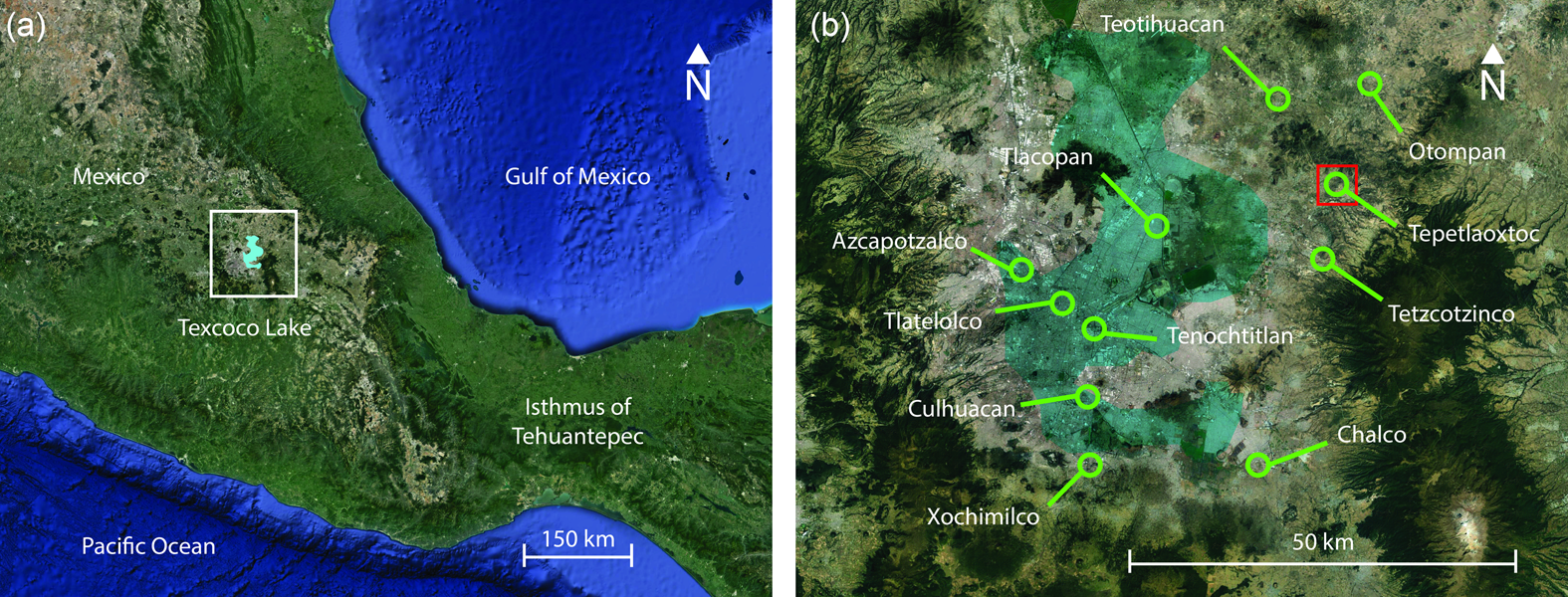
Figure 1. (a) Map of the central part of Mexico with an approximation of the shape of Texcoco Lake at the time; (b) the general area of the Texcoco Lake with indications of some of the most relevant places in the Acolhua confederation and in red, the location of Tepetlaoxtoc, the area of interest. (Color online)
The information contained in the codices is extremely rare and valuable. We argue that these codices give a glimpse into precolumbian proto-geometry and surveying. Surveying is an important state strategy that according to Scott (Reference Scott2008) did not occur in premodern states. Yet our analysis of the codices shows otherwise.
Our description and study of these codices are based on facsimile editions (Williams and Harvey Reference Williams and Harvey1997; Williams and Hicks Reference Williams and Hicks2011). The contents, writing, and drawings of both codices follow the same pattern and record agricultural fields of the same town, Tepetlaoztoc (also spelled Tepetlaoxtoc). These codices constitute prehispanic cadasters (land registers). They start with the population census of each household locality and then register the side lengths and areas of each of the agricultural fields that constitute the localities. Two sections of these codices are particularly important from the mathematical point of view: the milcocolli (to have turns, curves, or loops; Williams and Harvey Reference Williams and Harvey1997) section shows the approximate field shapes and side lengths of the fields, and the tlahuelmantli (smooth, leveled, equalized; Williams and Harvey Reference Williams and Harvey1997) section records the area of each field of the milcocolli (Figure 2). Although the codices have been known since the eighteenth century, it was not until 1980 that Harvey and Williams (Reference Harvey and Williams1980) deciphered the meaning of the tlahuelmantli. Our deep mathematical analysis was made possible by their work.
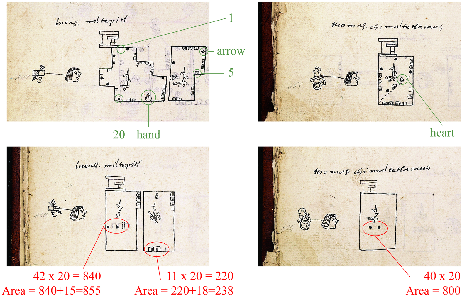
Figure 2. Example of milcocolli (top) and tlahuelmantli (bottom) records from CSMA.
The Acolhua used base 20 as did all Mesoamerican cultures (Closs Reference Closs1997). They had symbols for 1, 5, and 20 and three fractional units represented by a heart, arrow, and hand. There is no consensus on the values of the fractions, but Williams and Jorge y Jorge (Reference Williams and y Jorge2008) assign these values: heart = ⅖, arrow = ½, and hand = ⅗. The meaning of the number glyphs is shown in Figure 2. Using these values, it is straightforward to read the lengths of the sides shown in the milcocolli. For the top right field in Figure 2, the value on the dotted line is 25 + heart; starting at the bottom and moving clockwise, the values are 19, 35, 20, and 31 + 8 units. The unit of length was called tlalcuahuitl. The chronicle by Alva Ixtlilxochitl (Reference Alva Ixtlilxochitl and Chavero1952) describes the tlalcuahuitl (T) as the unit of length used in Texcoco, which is equivalent to 2.5 m. Due to the Texcocan origin of the codices, Harvey and Williams (Reference Harvey and Williams1980) used T in their important paper, as well as in all their subsequent work. We also use T in this article, as we did in our previous research.
Harvey and Williams (Reference Harvey and Williams1980) realized that the tlahuelmantli section contains records of areas. They also proposed how to read the numbers located in three different positions of those records. Numbers at the bottom or center of the rectangle (they never occur in both places) must be multiplied by 20, and the number in the tab is left as it is because it represents the units. Those two quantities are added to compute the area, as shown in Figure 2, bottom row.
The analysis of the vast number of fields in the codices has allowed us to make interesting observations about the Acolhua surveying records. Codex Santa María Asunción contains 971 records and Codex Vergara 618, for a total of 1,589 fields. However, not all the fields are legible, and not all of them have complete information; some fields have missing side lengths or recorded areas, and as noted, the CSMA has a whole locality for which there is only the tlahuelmantli section (the area records).
In our analysis, triangular fields and those with more than four sides are called N-polygons. In CSMA, there are 377 fields with only tlahuelmantli data, 50 quadrilaterals, 31 N-polygons with incomplete data, and one quadrilateral with impossible side lengths (one side is larger than the sum of the other three), giving a working corpus of 512 fields. In CV there is one field with only tlahuelmantli data, 21 quadrilaterals, 42 N-polygons with incomplete data, and one quadrilateral with impossible side lengths, giving a working corpus of 553 fields. We therefore present the analysis of the 1,065 fields with complete data.
Several important questions that are relevant from a mathematical standpoint arise from the codices: Where did the data in the tlahuelmantli come from, and were the fields measured or computed? And are the recorded measurements accurate? The answers are not obvious because side lengths alone do not determine the area in polygons with more than three sides, and there are no simple formulas for areas of irregular polygons. Additionally, measuring fields in situ can be very difficult, and the locations of most of the fields are unknown. We use algorithms and a computer program we created to provide some answers.
Measurement of Quadrilateral Fields
The majority of the fields (696) are quadrilaterals: 310 in CSMA and 386 in the CV. First observe in Figure 2 that the fields in the milcocolli are not drawn to scale, and there is no information about angles or diagonals; therefore, the shapes are misleading. Most of the depicted right angles cannot be right angles when the figures are drawn to scale. A very thorough mathematical examination of this corpus of 696 fields with complete data was possible because there are several mathematical tools to determine the areas of quadrilaterals, even irregular ones. Areas of irregular polygons with more than four sides and only side lengths specified are more difficult to study, but we wrote a computer program to compute them.
The applicable algorithm depends on the shape of the figure. The classification of the quadrilaterals by shape must be done through their side lengths and recorded areas because the images in the milcocolli are not reliable. For example, a field with four equal sides could be either a square or a parallelogram. We identify it as a square if the recorded area corresponds to the square of the side, which is the known area of a square. Equally, a quadrilateral with opposite equal sides is not necessarily a rectangle but could be a parallelogram. We identify it as a rectangle if its recorded area corresponds to base times height.
Using these definitions, we identified 91 squares and 45 rectangles, where the area recorded in the codices corresponds exactly to the base times height rule. This rule corresponds to dividing the quadrilateral into squares of unit side length whose area is 1T2; therefore, counting these unit squares will give the total area. This method sounds obvious today but was not always so.
It was only after 1857 when the metric system became the official measurement system in Mexico that standardized units began to replace the great variety of ambiguous units of land measurement. The Spanish brought with them variable units such as peonía, caballería, cuartillo, and many others. Although in 1536 Viceroy Mendoza established the dimensions of the caballería as 192 × 384 varas, in practice many parts of the land such as rocks or gullies were not counted. As a consequence, the land granted was much larger than it would have been had the official dimensions been used. Some other difficulties were variations in size of the vara and caballería in the different towns of New Spain; in addition, the caballería was sometimes calculated in terms of the fanegas de sembradura; that is, the number of seeds that could be planted on it (Carrera Stampa Reference Carrera Stampa1949; Gibson Reference Gibson and Campos1967).
Before the sixteenth century, the Acolhua developed the use of a surface unit defined as T × T = T2 = 2.5 m × 2.5 m = 6.25 m2 in land surveying to simplify the calculation of surfaces. This remarkable mathematical achievement represents an abstraction of the idea of the area. We do not know of any other Mesoamerican culture (and we would welcome any information from other researchers on this topic) that used a square surface unit—defined as a quadrilateral with its sides equal to one unit of length. Unfortunately, there is no evidence that T2 was still used during colonial times, representing another loss of prehispanic knowledge.
Codex Vergara
Previous work on the Codex Vergara has focused on its corpus of 367 legible records of quadrilateral fields. Williams and Jorge y Jorge (Reference Williams and y Jorge2008) argued that there is substantial evidence that the Acolhua used mathematical rules or algorithms to approximate the areas of these fields. They found five algorithms that reproduced 78% of the recorded areas exactly:
(1) Rule 1: Product of two adjacent sides
(2) Rule 2: Average of one pair of opposite sides times one of the other sides
(3) Rule 3: Surveyor's rule: product of the averages of opposite sides
(4) Rule 4: Triangle rule: divide the quadrilateral by one of the diagonals and sum of areas of the two triangles, assuming they have a right angle
(5) Rule 5: Plus-minus rule: add one (or two) unit(s) to one side and subtract one (or two) unit(s) from one adjacent side and multiply these new sides.
We illustrate each algorithm with examples in Supplemental Text 1.
After a thorough examination of the codex, we found 20 more legible fields that were not considered before, and thus the corpus of the database now consists of 387 quadrilaterals. The number of exact reproductions of the recorded areas using the five algorithms is 314 of 387, or 81.13% of the cases. This high percentage is due in part to the 123 square and rectangular fields in this codex.
There is evidence (92 fields) that the Acolhua used their fractional longitudinal units called monads (arrow, heart, hand) in the area approximations using these five algorithms. The fractional values given for these monads are still under review. To illustrate their use, consider the quadrilateral with side lengths of 18, 11, 19, and 12 and with recorded area of 222 from CV, locality 1, house 6, field 2. Using Rule 2, we take the average of the opposite sides 18 and 19 and multiply by 12. Since arrow = ½, then 2 × arrow = 1. Therefore, we write the average as (18 + 19) / 2 = 18 + ½ = 18 + arrow. Then the area is (18 + ½) × 12 = (18 × 12) + (½ × 12) = (18 × 12) + (½ × 12) = 216 + 6 = 222.
We also considered the accuracy of the surveying data. Given a quadrilateral with side lengths a, b, c, d, the maximum area it can enclose is given by (see Demir Reference Demir1966):

The first question we asked was whether the measurements in the codices are possible: Can the given side lengths enclose the given recorded area? A comparison with the maximum area provides the answer. If the recorded area is less than or equal to Amax, then there exists a field with the recorded measurements; however, if the recorded area is larger, then no field exists with the recorded measurements. For example, a quadrilateral with side lengths equal to 10 units can have any area between 0 and 100 square units, but no (flat) quadrilateral exists with side lengths equal to 10 units and an area larger than 100 square units. For this corpus, 137 fields (35.49%) were impossible (Jorge et al. Reference Jorge, Williams, Garza-Hume and Olvera2011).
In land surveying, however there are many sources of error. For instance, using the surveyor's rule (Rule 3) produces a result that is always larger than or equal to the maximum area. The percentage relative difference is defined as Pd = 100 × (Amax-Codex area)/Amax. When this quantity is positive, Amax is larger than the area recorded in the codex, and therefore the field is possible. These are the fields shown to the right of the zero line in Figure 3. When this quantity is negative, the area recorded in the codex is larger than the maximum possible area, and thus the polygon cannot exist mathematically.
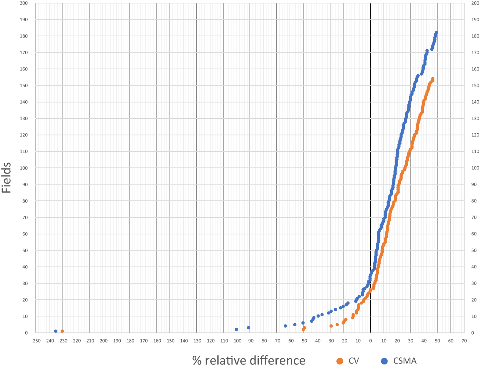
Figure 3. Percentage relative difference, Pd, shown for polygonal fields in both codices. Fields with a percentage relative difference larger than 10% are the ones we consider feasible. (Color online)
In real fields, one cannot expect perfect accuracy. As we did in an earlier article (Jorge et al. Reference Jorge, Williams, Garza-Hume and Olvera2011), we define a field as feasible if its percentage relative difference, Pd, is larger than or equal to −10%; that is, if it lies to the right of the −10% line in Figure 3 or if its percentage relative error is less than 10%. Our choice of 10% is arbitrary, but we believe it is reasonable. In CV, 99 impossible fields have relative errors less than 10% with respect to the maximum area, and therefore we consider them feasible; only 38 fields (9.81%) have a percentage relative error larger than 10%. Figure 3 shows a graph of the percentage relative difference in area for all the polygons with more than four sides in both codices. A few polygons have very large errors, which could be due to mathematical errors, measurement errors, errors by the tlacuilos (painters), or errors in the correspondence between milcocolli and tlahuelmantli. The fact that a polygon is feasible using this criterion does not prove that the recorded area is correct—only that it is plausible. However, the criterion does detect those fields that cannot exist.
Using elementary analytic geometry and a computer program to draw all the possible shapes of a quadrilateral, Jorge and colleagues (Reference Jorge, Williams, Garza-Hume and Olvera2011:File SI) proved that, given the four side lengths and the area of a possible quadrilateral, there are at most two different shapes (Garza-Hume Reference Garza-Hume2016; Garza-Hume and Jorge Reference Garza-Hume and del Carmen Jorge2018).
Codex Santa María Asunción
The first analysis of this codex was performed by Harvey and Williams (Reference Harvey and Williams1980). They approximated the areas of the quadrilateral fields by dividing them into two triangles and adding their areas. Assuming a right angle in the vertex formed by the base and the left side of each field, they used the Pythagorean theorem to find the area and the corresponding diagonal. Then they used Heron's formula (provided in the section on triangles) to calculate the area of the other triangle. Theirs was a first attempt to recover the recorded areas of quadrilateral fields in CSMA, and some of their calculations were very close to the recorded areas. From a mathematical point of view, however, their approach was very restrictive, because the angle between the first two sides is not necessarily 90°, and some quadrilaterals might not even have a right angle. When the angle between two sides is small, the approximation of the area is way too high, which explains the large size of some of their computation errors. Only in land plots that were rectangular or square were their approximations accurate (Figure 4).
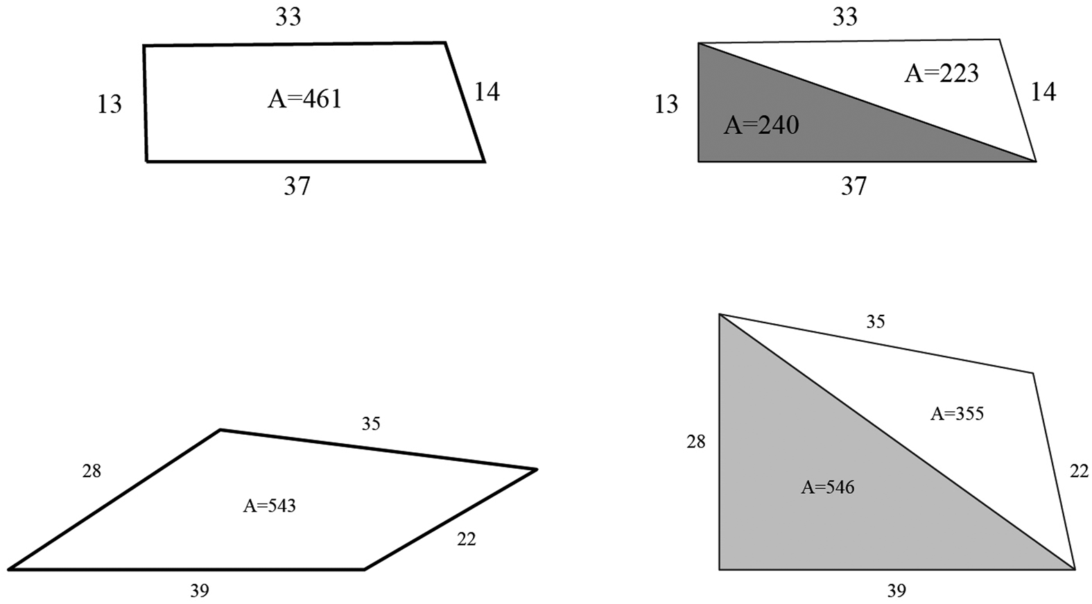
Figure 4. (Top left) A possible reconstruction and (top right) the area calculation using the Harvey-Williams algorithm, showing that the areas are very similar. (Bottom left) A possible reconstruction and (bottom right) the area calculation using the HW algorithm, showing the areas are very different.
We also applied the algorithms used in CV to CSMA, finding 137 cases in which the areas are exactly reproduced. For a corpus of 310 quadrilaterals with complete data, this represents 44.19% of the cases, a lower percentage than the 80.87% of the CV. This lower percentage may have been due to our identification of only one square and 12 rectangular fields. A total of 172 quadrilateral fields could not be approximated with these algorithms, and we have not been able to find new ones that enable good approximations. We therefore speculate that the Acolhua applied surveying methods that cannot be put into algorithms. Perhaps they made a grid in each field or divided the field into regular shapes and then added their areas.
In CSMA there is also evidence that fractions were used in the computations. The algorithms tested for CV yield zero error in 59 cases from CSMA when fractions are considered.
We calculated the maximum areas for all the quadrilaterals and compared them with the recorded areas to test for feasibility. There were 193 (62.25%) impossible fields, a higher percentage than for CV. However, 135 fields have a relative error less than 10% with respect to the maximum area, and therefore only 58 (18.7%) fields are unfeasible. As mentioned earlier, CSMA is not very well preserved. Some parts are damaged, and 377 fields only have tlahuelmantli data. If the document was complete, maybe the statistics would be more favorable. The two possible shapes of the quadrilaterals and the maximum area shape for all fields were obtained with the same program designed for CV.
Shapes of the Fields
For the quadrilaterals, we identified some of their shapes according to their recorded area, rather than from the depiction in the codices. The pictures of the fields in the milcocolli section are not a reliable guide, because the tlacuilo tended to draw right angles in most of them and the sides are not drawn to scale. When we reconstructed the shapes, we found many quadrilaterals that could not have a right angle between the first and second sides. An example is a field with sides 15, 15, 39, and 39 T. There is a configuration with a right angle between the two short sides, but it is impossible to have a right angle between the two long sides (see Figure 5).
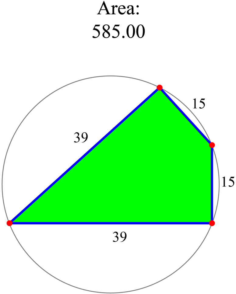
Figure 5. It is impossible to have a right angle between the two long sides.
Squares, rectangles, and parallelograms are the easiest shapes to recognize from the data of the milcocolli and tlahuelmantli. The squares not only have to have sides of equal length, but their area must be the square of the side; if this condition is not satisfied, the shape is a parallelogram. Likewise, the rectangles must satisfy not only the criterion that the opposite sides are equal but also the area is equal to the product of two adjacent sides: base × height. Otherwise, the shape is a parallelogram.
Regular Trapezoids
There are 65 fields in the codices (37 in CSMA and 28 in CV) with two equal sides. In all of these fields, the recorded area is greater than the maximum area. We found a new algorithm that reproduces the recorded area of these fields: an average of unequal sides times the other side. Since the actual formula to calculate the area of a trapezoid is an average of parallel unequal sides times height and this gives the maximum possible area of the quadrilateral, we compared the recorded areas with the trapezoid areas. We found that in 35 cases the error is less than 1%, and in the rest, it is less than 10%; therefore, according to our criterion they can be considered feasible. Moreover, there are 24 cases in CV and 24 cases in CSMA where the height is so close to the sides of equal length that the error between the recorded area and the maximum area is nearly zero. The example shown in Figure 6 has side lengths 31, 20, 25, and 20. The recorded area is 560 T2, which coincides with (31 + 25)/2 × 20. The maximum possible area is 553.66 T2.
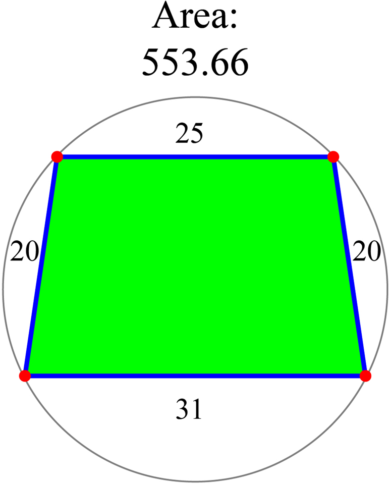
Figure 6. Trapezoid with side lengths 31, 20, 25, and 20 T in its configuration with the maximum area of 553.66 T2.
Rhombuses
This kind of quadrilateral has two pairs of adjacent equal sides but of different lengths. The data from the codices are shown in Table 1. There are three rhombuses in CV, all of which are unfeasible, and three in CSMA, one of which is feasible and two are unfeasible. Some of the errors with respect to the maximum area are very high. We mention them because the recorded areas in the codices for five of these quadrilaterals are impossible to recover using any algorithm. It remains a puzzle to discover how those area records were calculated.
Table 1. Side Lengths and Areas of Rhombuses from both Codices.
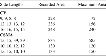
The configuration with the maximum area for rhombuses has two right angles located between the sides with different length; given that the angles are equal, their sum must be 180 degrees. The first one from CMSA is depicted in Figure 5 in its configuration of maximum area.
Triangles
We were also puzzled by the recorded areas for the triangles. Only three fields of this shape appear in the codices: two in the CV and one in CSMA with no recorded area. The exact area can be calculated using Heron's formula: for a triangle with side lengths a, b, c,

This formula requires the computation of a square root, and there is no evidence that the Acolhua knew how to do that. None of the triangles in CV are feasible: one of the recorded areas is 13% larger than the exact area, and the other is 230% larger. Williams and Jorge y Jorge (Reference Williams and y Jorge2001) proposed an algorithm to approximate the area, explaining the overestimation of the area of the second triangle as caused by a possible missing dot in the milcocolli record.
As we mentioned earlier, the Acolhua calculated the area by counting how many unit squares of size T2 = 6.25 m2 are inside the field. Therefore, it is plausible that the calculation of the field areas in situ was performed using a sort of net to create a mesh of squares over the measured field.
Polygonal Fields
We now proceed to analyze the fields of the CSMA and the CV with more than four sides, which we refer to in this section as polygons. As one might expect, extending the ideas used in the analysis of the quadrilateral fields to polygon is complicated.
CV has 209 polygons with the number of sides ranging from 5 to 19, and CSMA has 233 polygons with 5–23 sides. Not all the data are given, some polygons have missing side lengths, and some have no record of the area. There are 42 fields with incomplete data in CV and 31 in CSMA. The total corpus consists of 167 in CV and 202 in CSMA, giving a total of 369 polygonal fields.
It is possible to find the configuration with the maximum area for any polygon: it is the one that can be inscribed in a circle (Demir Reference Demir1966). Nevertheless, the shape of this polygon may be very different from the usual shape of an agricultural field, as can be seen in Figure 7. To test for feasibility, we again compared the recorded area with the maximum area, which in this case is the area of the inscribed polygon shown in the figure. In CV there are 25 impossible cases, and 12 have an error of less than 10%; therefore, there are only 13 unfeasible fields. In CSMA there are 34 impossible cases and 14 have an error of less than 10%; therefore, there are 20 unfeasible fields. Again, the numbers in the CV are better than the ones in CSMA. A total of 336 polygons in both codices are feasible.
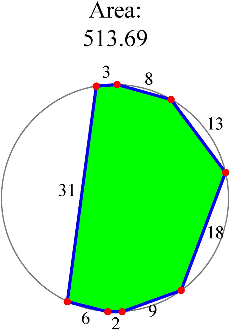
Figure 7. Configuration with the maximum area.
Given five or more different side lengths and a possible area—one between the minimum and the maximum areas for the given side lengths—there is an infinite number of shapes. This makes the reconstruction of the shapes of the fields very difficult. However, following the pictures of the milcocolli, it is possible to select a few likely shapes. To do so we designed a computer program that uses JSXGraph (see Garza-Hume Reference Garza-Hume2016; Garza-Hume and Jorge Reference Garza-Hume and del Carmen Jorge2018) and is very easy to use. After the user enters the sides and area of the polygon, it gives the configuration with the maximum area (which is unique) and allows the user to deform it by dragging the vertices.
The first problem one faces when trying to reconstruct the milcocolli shapes, apart from the fact that the number of possible configurations is infinite, is the large number of right angles contained in the drawings; most of them are not possible if one wants to achieve the area given in the tlahuelmantli. Therefore, whether to retain a certain right angle shown in the codices is a decision of the program user, who must consider the fact that the sides are not drawn to scale and that the right angles are probably due to the tlacuilo's style. In Figure 8 we present two reconstructions drawn with the program we designed. They are both from CV: the one on the bottom left is 01-04-01, and the one on the top left is 01-01-01 in our database (f.6v in the online version at the Bibliothèque Nationale de France). When drawn to scale the figures only resemble those in the codex. Note that when using our program, we can only recover approximations of recorded areas because moving one vertex moves all the others to preserve the side lengths. Thus, it is very difficult to control the area exactly.
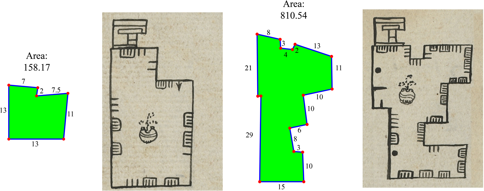
Figure 8. Possible reconstructions of fields from CV.
Finding algorithms that approximate the recorded areas for the polygons is a very difficult task because there are more quantities to combine; so far, we do not have a systematic way to approximate the recorded areas of fields with large numbers of sides. We do, however, have a few good approximations for some fields with five or six sides. The fields with six sides are the most common and the most suitable ones to test for possible area algorithms. One idea is to divide the field into quadrilateral parts and add the corresponding approximations of the areas. Field 01-04-01 in Figure 8 is a good example: its area can be approximated as the sum of two rectangles: 13 × 11 + 7 × 2 = 157. Another idea is to enclose the field into a larger quadrilateral and subtract the area of the smaller one. More examples can be seen in Williams and Jorge y Jorge (Reference Williams and y Jorge2001) and in Figure 9.
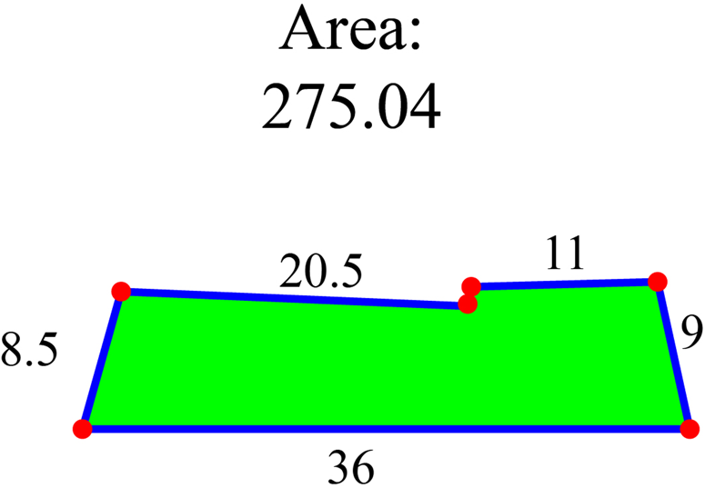
Figure 9. This image corresponds to field 01-04-002 in the CV. Side lengths are 36, 8.5, 20.5, 1, 11, and 9 T. The recorded area is 275 T2. It can almost be recovered as 20.5 × 8.5 + 11 × 9 = 273.2, the sum of the approximate areas of the left and right quadrilaterals.
Unfortunately, we were unable to reconstruct the area for most of the cases that we studied using our algorithms. The areas of fields with five sides are more difficult to calculate, and as the number of sides increases, the task becomes more daunting. We have not yet found an algorithm that works for all the polygons, and one may not even exist. It is possible that the areas of polygonal fields were measured and not computed by the Acolhua.
Comparison with Satellite Data
Topotitla, Locality 2 in CV, is a locality in the codices whose geographic position is known (Rojas et al. Reference Rojas Rabiela, López and Lima2000; Williams and Hicks Reference Williams and Hicks2011). The field is roughly triangular with an old-looking walking path on the west border, the remains of an ancient wall on the northwest, and a stream on the eastern border. It is still in use as an agricultural field, which made it easy to measure enough GPS coordinates on its boundary to calculate its satellite area and compare it with the total area registered in CV (Jorge et al. Reference Jorge, Williams, Garza-Hume and Olvera2011). The details can be seen in Appendix 1.
The locality has 38 fields: 24 quadrilaterals and 14 polygons. Three quadrilaterals and one hexagon have missing tlahuelmantli; we used their maximum areas to approximate the area of Topotitla as given in the codex. The total area in CV is 135,577 m,2 and the satellite measurement is 124,071.52 m2. The difference of 11,505.48 m2 means that the Acolhua measurement is 9.27% greater than the satellite measurement. Recall that these computations were done assuming T = 2.5 m; the fact that this difference is so small for field measurements gives more evidence that this is the correct value of T.
We can now improve the previous approximation using our software to draw shapes and find areas. The hexagon with missing tlahuelmantli (CV, p. 23v) has a maximum area of 637 T2, the value used in Jorge and colleagues (Reference Jorge, Williams, Garza-Hume and Olvera2011). However, if we use our software to approximate the field shape given in CV with the side lengths registered in the milcocolli, it gives an approximate area of 482 T2: a difference of 155 T2, or 968.75 m2 less than the CV area reported in Jorge and colleagues (Reference Jorge, Williams, Garza-Hume and Olvera2011). Thus, the total approximated area in CV is now 134,608.25 m2, and the difference of 10,536.73 m2 in ground measurement represents an Acolhua area that is 8.49% greater than the satellite area. If we consider that there are three quadrilaterals in Topotitla without tlahuelmantli records that were approximated with their maximum area, we can expect that the excess Acolhua area was less than 8.49%. Figure 10 shows the codex drawing, the shape given by our program, and the maximum area approximation used in Jorge and colleagues (Reference Jorge, Williams, Garza-Hume and Olvera2011).

Figure 10. Drawing from the codex: reconstruction is used for the computation and configuration with the maximum area. The recorded area is 482. We could not recover it exactly but only approximately.
The ground measurements reported by Jorge and colleagues (Reference Jorge, Williams, Garza-Hume and Olvera2011) used a Lambert plane projection of the surface. Considering the shape of the earth, the measurements were improved using the Quantum Geographic Information System (QGIS). In this case, 103 coordinates on the border of Topotitla were used together with a Pseudo Mercator projection. The calculated area is now 131,059.5 m2, which is closer to the codex area. Another comparison was made using Google Earth Pro, which uses a projection on a cylindrical plate and a rough elevation model; in this case, the calculated area is 130,088 m2. These methods are more refined than the one we used previously (Jorge et al. Reference Jorge, Williams, Garza-Hume and Olvera2011), and it is interesting to observe that these areas are closer to the CV area, reinforcing our confidence in Acolhua surveying methods. Supplemental Figures 1 and 2 show the Topotitla locality and the coordinates used in the approximations. The fact that the eastern border of Topotitla is a stream and hence could have moved over the centuries suggested that we could jiggle this border slightly east or west. When we did this, the surface area varied approximately between 120,000 m2 and 135,000 m2.
Both facsimile editions of the codices contain a rough idea of the location of the fields contained in them. The approximate site of two of the five localities in CV were found previously on an old map and identified by soil type; in addition, property titles were discovered by several researchers. Barbara Williams reconstructed a map of Calla Tlaxoxihuco showing the fields registered in the codex with their soil type (Williams and Hicks Reference Williams and Hicks2011). Topotitla's location was identified by several researchers. For CSMA, Johnson (Reference Johnson2018) gives a proposed reconstruction of some fields in the localities of Cuauhtepuztitla and Tlanchiuhca. This result can be used as a starting point to perform fieldwork aimed to repeat the analysis done in Topotitla.
Conclusions
In this work, we extended some results from CV to CSMA and added some improvements. We presented the analysis of polygons with more than four sides.
The first and most important concept contained in the codices, from a mathematical point of view, is that the surface unit is the area of a square of one unit of length. This represents a high level of abstraction in mathematical thinking; it reduces the action of measuring surface area to a simple counting of unit squares contained in it. The idea that there exist simple algorithms to approximate the area is equivalent to finding different ways to count the squares included entirely or in part in a given region.
Our analysis corroborated the value of T as 2.5 m or 3 varas, as given in Alva Ixtlilxóchitl (Reference Alva Ixtlilxochitl and Chavero1952), by comparing the satellite measurement of Topotitla to its total recorded area in CV: that comparison gives a difference of 8.49%. If T were 2 varas or 1.67 m, as seen in Tenochca documents, the area in the codex would be 58,280.52 m2, and the difference with the satellite measurement would be 53%.
We constructed a database for each codex that includes very thorough information about their content. These two databases enabled us to create a detailed description of each agricultural field that includes these elements: location, side lengths, recorded area, maximum area, calculations with the algorithm used to approximate the area, fractions, reconstruction of shape, and feasibility. We created a web page for Acolhua surveying where these databases can be found (see Garza-Hume and Jorge Reference Garza-Hume and del Carmen Jorge2018). The page also contains relevant information on this topic.
Although the algorithms we proposed to calculate quadrilateral areas worked very well with the CV fields (80.87% reproduced with the algorithms), the results were less than half as good (44.19%) in the case of CSMA. We experimented with various algorithms but were unable to find any that reproduced most of the recorded areas. It seems that in CSMA other types of algorithms to calculate areas were used or the fields were measured in situ. It is still not clear whether the Acolhua measured or computed areas. It would be very interesting to analyze the quadrilateral fields of this codex with a different perspective.
With the large available corpus of agricultural fields, an important question arose: Can we determine whether the given side lengths really enclose the recorded area? The answer is a definite yes. Given the side lengths of the milcocolli section, Jorge and colleagues (Reference Jorge, Williams, Garza-Hume and Olvera2011) found a mathematical tool to compute the maximum possible area for quadrilateral fields in CV; then they compared it with the area given in the tlahuelmantli to conclude that when the maximum area was less than the recorded area, that field was impossible. This a very important tool because it is precise. However, based on Atwell (Reference Atwell1665), Earle (Reference Earle1975), Kain and Baigent (Reference Kain and Baigent1992), Bower (Reference Bower2009), and Nickel (Reference Nickel2010), Jorge and colleagues (Reference Jorge, Williams, Garza-Hume and Olvera2011) considered that a percentage relative error less than 10% was acceptable, and they proposed to call such fields feasible.
In this work we applied this concept to polygonal fields from both codices to find the percentage of unfeasible fields. The feasibility test for CV found that 9.8% of quadrilaterals were unfeasible versus 18.7% for those in CSMA. We cannot rule out that the condition of CSMA, with its missing or illegible sections, could be the cause of the difference in the percentages. There are very few unfeasible polygons: 13 (7.78%) in CV and 20 (9.9%) in CSMA. The low percentage of unfeasible fields in both codices is remarkable considering that the records are almost five centuries old and the instruments to measure an agricultural field were most likely ropes and sticks. With this evidence we conclude that the Acolhua were very good surveyors.
We analyzed polygons with more than four sides in both codices and tried various algorithms to recover the areas given in the codices but were not successful in doing so. This remains an open problem.
Our computer program allows the approximate reconstruction of the shapes of the fields (Garza-Hume Reference Garza-Hume2016; Garza-Hume and Jorge Reference Garza-Hume and del Carmen Jorge2018). The satellite measurement of Locality 2 of CV, Topotitla, was improved using the software QGIS: the new approximation of its surface area is closer to its total area recorded in the codex. It would be very interesting to study other localities with a proposed geographical location such as Calla to compare between codex data and satellite data. Our program that reconstructs shapes might be a useful tool here.
We consider these codices to be invaluable sources for the study of ancient land surveying methods in Mesoamerica before European contact. With the concept of the square measure, the Acolhua surveyors used both practical and abstract thinking to develop a very straightforward way to deal with surface measurements. Unfortunately, it was not recognized by the Spanish and drifted into oblivion for more than four centuries.
Acknowledgments
We thank Ana Perez Arteaga for her invaluable support with the databases and web page and the reviewers for their very pertinent comments. The authors have no conflicts of interest.
Data Availability Statement
Códice Vergara can be seen online at the Bibliothèque Nationale de France (https://gallica.bnf.fr/ark:/12148/btv1b84528032.image). Códice Santa María Asunción was edited by B. J. Williams and H. R. Harvey and published in 1997 as The Códice de Santa María Asunción: Households and Lands in Sixteenth Century Tepetlaoztoc (University of Utah Press). Databases with a summary of the information from both codices can be seen at http://agrimensuraazteca.iimas.unam.mx.
Supplemental Material
To view supplemental material for this article, please visit https://doi.org/10.1017/laq.2021.58.
Supplemental Text 1. Algorithms to approximate areas of irregular quadrilaterals.
Supplemental Figure 1. Zoom-fit to the zone of interest defined by the vector layer containing polygon geometry with 103 connected vertices placed over highly recognizable terrain limits and prominent contour terrain features of the Google satellite layer.
Supplemental Figure 2. Screenshot of the Google Earth desktop package visualization over the zone of interest after importing the KML file previously exported from the vector layer in QGIS.
Appendix 1
The Topotitla zone of interest was defined using an ESRI (Environmental Systems Research Institute data format) shapefile vector layer inside the open-source Quantum Geographic Information System QGIS 3.2.2 (Bonn); the shape layer contains a nontopological polygonal dataset of 103 connected vertices obtained by placing anchor points over recognizable terrain limits and prominent contour terrain features at a 1600% zoom over a high-resolution Google satellite imagery layer at 1:5000 scale; both layers were georeferenced using the European Petroleum Survey Group, Geodetic Parameter Dataset, World Geodetic System 84 (EPSG:3857/WGS84) Pseudo Mercator projection (a spherical development of an ellipsoidal coordinate system using an auxiliary sphere), compatible with Google mapping and other popular geographic visualization applications. The perimeter and area calculations were performed using the QGIS identify object built-in function over the vector layer; according to these calculations, the zone of interest has a perimeter of 1,713.597 m (Cartesian) / 1,609.103 m (ellipsoidal) and an area of 146,897.967 m2 (Cartesian) / 131, 059.5 m2 (ellipsoidal).
Afterward, the vertex layer was exported to a KML file format for comparison with Google Earth Pro 7.3.2.5491, which also uses WGS84; however, instead of a Pseudo Mercator projection, Google Earth uses a cylindrical plate and a rough elevation model. The polygon's vertices were dropped to the local ground level (2,325 m), and the built-in object properties calculations for perimeter and area were performed; the results over the defined polygon were 1,609 m for the perimeter and 130,088 m2 for the area.
Even when the results of the perimeter calculation in both applications are equal, there is a difference of 971.5 m2 in the area calculation due to the use of two different projection methods (QGIS, ellipsoidal versus Google Earth, cylindrical) and the use of a rough 3D elevation model in Google Earth versus the slightly deformed—toward the north—flat 2D layer in QGIS; the QGIS calculation yields a slightly larger area. Nevertheless, the difference in the results with both area calculations is relatively small, and the numbers are consistent with the information previously obtained by the GPS field survey in the area. Two images can be seen in Supplemental Figure 1 and Supplemental Figure 2.


