1. INTRODUCTION
High-power lasers provide possibilities to study different aspects of
astrophysical phenomena in the laboratory (Remington
et al., 2000; Ryutov et
al., 2001). Recent advances in generating ultrashort laser
pulses with intensities far beyond 1018 W/cm2
(Strickland & Mourou, 1985; Mourou et al., 1998) allow us to access
new regimes of relativistic electron beams (REB) carrying huge currents
and magnetic fields (Pukhov & Meyer-ter-Vehn,
1996; Tatarakis et al.,
2002). Here we study the excitation of large-amplitude plasma
waves (Langmuir waves) by laser-generated relativistic electron beams
and their emission of electromagnetic radiation at multiples of the
plasma frequency. Such emission was discussed long ago (Aamodt & Drummond, 1964); it has been observed
in solar type III radio bursts where two bands of emission are found
that are interpreted as fundamental and second harmonic plasma emission
driven by Langmuir waves (e.g., Melrose et
al., 1986). The detailed models for the ratio of
fundamental and harmonic emission and the absolute intensities are
still under discussion (e.g., Vasquez et
al., 2002).
The two configurations of the laser experiment and the solar corona
are sketched in Figure 1. Different REB
sources have been used to make plasma waves in the laboratory (Vyacheslavov et al., 2002). Here we
investigate a p-polarized laser pulse focused to relativistic
intensity on a thin overdense plasma layer (see Fig.
1a). With the period of the laser light, it produces electron
pulses that start to oscillate through the foil. They have current
densities of the order of 1012 A/cm2. The
pulses generate counterpropagating plasmons and subsequent radiation at
multiples of the plasma frequency. This process will be described in
detail below.
a: Schematic drawing of the laboratory configuration investigated in
this article. b: Schematic picture of the standard model for solar type
III radio bursts.
In the solar case (see Fig. 1b), these
energetic electrons are generated near the solar surface by magnetic
reconnection, a process releasing energy of a twisted magnetic field by
sudden reconnection of the magnetic field lines. Small scale magnetic
fields near the solar surface are constantly twisted as the sun rotates
differentially. Reconnection events on small time and space scales take
place frequently and are stochastically distributed. The fast electron
beams move through the coronal plasma and excite Langmuir waves
triggered by two-stream instability. An important point is that the
waves are first created in a forward direction, but quickly scatter on
ion polarization clouds so that the growth rate of the instability is
strongly reduced. This leads to an almost isotropic distribution of
Langmuir waves in the excitation region, which is believed to extend
over 2 solar radii or 1.4 million km.
The radio emission occurs when two or more plasmons decay into a
photon. The simplest process is two-plasmon decay obeying the matching
conditions
where ωp =
4πe2n0 /m is
the plasma frequency with electron density n0,
charge e, and mass m of the electron. Because the
plasmon wave vectors k1 and k2
are typically much larger than the photon wave vector
kT, they have to be approximately
antiparallel, implying counterpropagating waves. The photon energy is
ωT ≈ 2ωp. Higher
order processes involving more plasmons may lead to radiation also at
other multiples of ωp. When probing the sun in
the radio frequency range, one observes transient features of coherent
radio emission. The signal starts at a frequency of about 100 MHz and
stays on for some 10 s, during which the frequency gradually declines.
In many cases, a second frequency band of almost equal intensity can be
traced, which suggests that the two bands represent emission at the
fundamental and the second harmonics of the plasma frequency. The
decreasing frequency indicates that the radiation source travels
outward in the solar corona into regions of lower electron density and
therefore smaller plasma frequency. The measured time scales are
consistent with such a picture, taking the source as a beam of mildly
relativistic electrons with a velocity of about 40% of the speed of
light.
Experimental evidence for 2ωp emission from
laser-irradiated materials has been reported (Teubner et al., 1997), but more
experimental work seems necessary to substantiate these results. The
intention of the present article is to give a basis for such
experiments by means of one-dimensional particle-in-cell (1D PIC)
simulation, using the code LPIC++ (Lichters et
al., 1997). First results of this work had been reported in
1998 (Lichters et al., 1998). It
uses kinetic simulation of laser plasma interaction at the target
surface, describing hot electron transport through the foil, plasmon
excitation by two-stream instability, and two-plasmon decay into
photons.
The simulation considers only one spatial dimension (i.e., all
physical quantities depend on x and t, but not on
y or z). However, it takes into account all three
velocity components, and therefore allows us to treat oblique incidence
of arbitrarily polarized laser beams. Oblique incidence is treated by
transforming into a boosted frame in which the laser beam is normally
incident on a moving foil. Details of this Lorentz transformation are
described in Section 2 and the evolution of electron phase space in
Section 3. Section 4 is devoted to an analysis of plasmon distributions
in x, t space and k, ω space and their
decay into photons at multiples of the plasma frequency. In Section 5,
the 2ωp emission is treated analytically on
the basis of the cold fluid approximation.
The restriction to one spatial dimension represents a severe
limitation of the present treatment for two reasons. First, it excludes
surface plasma waves that are certainly also excited and couple through
nonlinear terms to the electromagnetic spectrum (Ivanov & Ryutov, 1965; Ryutov, 1966). Second, the transverse distribution
of laser intensity and light pressure over a focus of finite size leads
to crater formation, destroying the planar target geometry. Third, the
fast electron current driven into the foil is subject to transverse
Weibel instability, leading to current filamentation, which cannot be
described in the present 1D treatment. These phenomena clearly show up
in 2D and 3D PIC simulation (see, e.g., Pukhov &
Meyer-ter-Vehn, 1997; Honda et al.,
2000). To mitigate these effects, we restrict the present investigation
to very short, few-cycle laser pulses, which have now become available
experimentally (Brabec & Krausz, 2000),
and consider configurations with a focal diameter large relative to
target thickness, in which planar geometry should prevail over a longer
period. The influence of current filamentation with a spatial scale of
c/ωp on plasmon excitation is
more difficult to judge and certainly needs future multidimensional
investigation. Nevertheless, we believe that the present 1D results
give a qualitatively valid picture and a basis for stimulating
experiments.
2. OBLIQUE LASER INCIDENCE IN 1D
DESCRIPTION
The numerical results shown in the subsequent sections have been
obtained with the 1D PIC code LPIC++. This code is documented and
freely available (Lichters et al.,
1997). The code simulates the interaction of strong, ultrashort
laser pulses with thin plasma layers and allows for a self-consistent
treatment of electrostatic and electromagnetic waves. Oblique incidence
of the laser pulse is included in this 1D description by means of a
Lorentz transformation into a moving frame, in which the light is
normally incident on the layer (Bourdier,
1983). This transformation is possible because the code
considers three velocity and field components, though only one spatial
coordinate. It also allows us to study arbitrary polarization. In the
present simulations, the material layer is assumed to be fully ionized
initially.
The interaction of the laser pulse with the plasma layer is treated
in the frame L′ illustrated in Figure
2. For p-polarized light, only the propagation
direction x and the polarization direction y are of
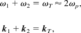
importance. The wave vector of the incident light in the laboratory
system L
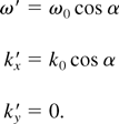
transforms to the moving system L′ according to
where Γ = sec α is the Lorentz factor corresponding to the
velocity β = vy /c of the
frame in positive y direction. For β =
ky c/ω0 = sin
α, one has
In this boosted frame, the 1D laser plasma equations in the cold
fluid approximation have the form (Lichters, 1997)
where we used normalized quantities for the amplitude of the vector
potential ay =
eAy /(mc2), the
electron density n = ne
/n0, the electrostatic potential φ =
eΦ(mc2), and the x component
of the fluid velocity βx =
vx /c. Here we have assumed
p-polarized light, that is, ax =
0. In linear approximation, these equations allow for electrostatic
(Langmuir) waves
with ω = ωp cos α and arbitrary
k. In addition, light waves
can propagate with the usual dispersion relation ω2 =
ωp2 + (ck)2.
Notice that, in the boosted frame, the fields
ay(x, t) and
φ(x, t) are coupled to each other such that, for
example, electrostatic waves are not purely longitudinal, but have an
Ey component for α > 0.
Schematic view of the simulation geometry for a p-polarized
laser pulse. In the laboratory system L the target plasma is at rest,
and the laser pulse is incident under an angle of α; in system
L′ the plasma moves uniformly with velocity
v/c = −sin α in y direction
such that the laser shines on the foil perpendicularly.
The code LPIC++ solves the set of nonlinear Eqs. (4) numerically. In
this article, we present simulations of a p-polarized laser
pulse incident under an angle of α = 55° on a plane layer of
overcritical, fully ionized plasma with sharp boundaries. The angle is
chosen to optimize 2ωp emission (see Section
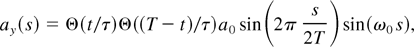
4). The pulse shape is
with s = t − x/c, τ
= 2π/ω0, and Θ(x) is the
Heaviside step function. A short pulse T = 4τ is chosen.
The plasma density is n0 =
18nc, where
nc =
πmc2/(e2λ02)
is the critical density and λ0 =
2πc/ω0 the laser wavelength. two layer
thicknesses d are considered:
- d = 1λ0 (the “thin foil” case)
and
- d = 5λ0 (the “thick foil”
case).
The laser amplitude is taken as a0 = 2 in both
cases and corresponds to an intensity of I = 5.5 ×
1018 W/cm2 for 1-μm laser wavelength.
3. GENERATION OF FAST ELECTRONS
The laser pulse itself cannot penetrate into the overcritical plasma
layer. The excitation of plasma waves inside the layer is mediated by
fast electrons, which are accelerated to relativistic energies by the
laser field at the surface. For a p-polarized laser pulse
obliquely incident on a plasma surface, there are two mechanisms that
drive the fast electrons:
- The light pressure normal to the surface that originates from the
v × B force; it is of second order in the light
amplitude and therefore oscillates with twice the laser
frequency;
- The direct action of the laser electric field normal to the foil
that pulls electrons off the surface, accelerates and reinjects them
into the plasma periodically at laser frequency (vacuum heating; Brunel, 1987). This force is linear in the laser
amplitude and is therefore the dominant process for laser intensities
up to 1018 W/cm2.
Different groups of fast electrons (called jets in the
following) are observed in the phase space plots of Figures
3, 4, 5, and 6, showing
vx and vy
distributions in the laboratory system. In Figure 3,
vx is plotted versus x for a plasma
layer located at 3 < x/λ0 < 4. The fast
electrons are generated close to the surface and disperse according to their
velocity spectrum when penetrating into the plasma layer. After 4 laser
periods (left side of Fig. 3), one observes a first
jet that has spread over the full layer thickness and a second one just
being formed at the left surface. Bulk plasma electrons at low velocity
are seen to carry a large-amplitude plasma wave. Apparently, the first
jet has excited this wave, which is acting back on the jet, modulating
its velocity spectrum. After eight laser periods (right side of Fig. 3), the phase space looks more complicated.
One now observes fast electrons at x/λ0
> 4 beyond the right surface, where they build up a negative charge
cloud, and electrons with vx < 0, which
have been reflected by this space charge and are now running from left
to right. In addition, we recognize a dense band of electrons with
velocities vx > 0 in a range
vx /c ≈ 0.05–0.25.
It appears that this electron group has also been heated by the peak of
the laser pulse, but in deeper parts of the skin layer leading to a
broader distribution at lower velocity as compared to the jet
electrons.
Phase space diagrams of electron velocity
vx for a 1λ-thick foil with
n/nc = 18 and a laser pulse
incident from the left with a0 = 2 and α = 55
after t/τ = 4 (left side) and t/τ = 8
(right side) laser periods. While all high-velocity electrons are
plotted, those belonging to the bulk plasma with high electron density
are partially suppressed.
Same as Figure 3, but for
vy.
Phase space diagrams for vx for a
5λ0-thick foil after t/τ = 6 (left
side) and t/τ = 15 (right side); plasma and laser
parameters are the same as in Figure 3, and
τ is the laser period.
Same as Figure 5, but for
vy.
In Figure 4, the corresponding
vy versus x plots are shown.
Different from vx, only electrons with
positive vy component are found inside the
layer. This is a consequence of the oblique laser incidence. Inside the
layer, the vector potential analysis vanishes, and the
transverse electron momentum in the moving frame is
where βx′ and
βy′ are the velocity component in
L′. Using the relations
for the velocity transformation
between the frames L′ and L with relative velocity β = sin
α, one obtains for the laboratory velocities
showing that vy > 0 for α =
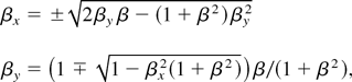
55°. Equations (14) also imply upper limits for
βx and βy depending on
α. For α = 55°, one finds βx ≤
0.774 and βy ≤ 0.819, which is in good
agreement with the maximum velocities seen in the phase space plots.
Some aspects of the electron evolution discussed above appear even
more pronounced for a thicker layer with d =
5λ0, leaving all other parameters unchanged. This is
shown in Figures 5 and 6. At time t = 6τ, one now sees three
jet and the onset of a fourth one without interference of reflected
electrons, as the jet travel time through the layer is longer.
Reflected electrons populating the vx <
0 plane are seen on the right side of Figures 5 and 6, showing the
phase space at t = 15τ. At this later time, one also very
clearly observes the band of medium velocity electrons, clearly
separated in phase space from both jet and plasma electrons.
The electron density n(x, t) corresponding
to the thin layer plots in Figures 3 and
4 is shown in Figure
7. It refers to the laboratory frame. The gray scale applies to
the density inside the layer, while fast electrons outside the plasma
are marked by black dots. The plot shows impressively the electron
excitation by the laser pulse. At early times, one should notice the
electrons pulled out from the irradiated left surface and then
reinjected into the layer with period τ. Superimposed on the direct
action of the laser electric field is the action of the ponderomotive
pressure with the period τ/2. The electrons pass the layer and
emerge from the right-hand side. Due to space charge build-up, they
cannot escape from the layer in large amounts, but rather return and
then oscillate back and forth through the layer, where they excite
plasma waves seen as density ripples inside the layer. Notice that also
the electron group of intermediate velocity excites plasma waves,
weakly seen as steep lines in Figure 7. The
steepness corresponds to lower phase velocity.
Electron density n(x, t) plotted in
x, t plane. Inside the foil, the gray scale has been
selected to highlight the density oscillations around the initial
density n/nc = 18 in the
range of ne
/nc = 14–20. To also visualize
laser-driven electrons of much lower density escaping the layer on both
sides, each cell in this region with
n/nc < 80 has been
indicated by a black dot except for cells with zero density, which
remain white.
The density profile is also plotted in Figure
8 as a snapshot at time t = 5τ, showing details of
the space charge distribution in front of the rear surface. Here the
electron density amounts typically to 2% of the critical density and
reaches 10% at the right border.
Electron density n(x, t) plotted versus
x for t = 5τ. The scale has been chosen to show
the density distribution in front of the rear surface; notice that it
is modulated with the plasma wave period.
4. PLASMON GENERATION AND RADIATION AT
MULTIPLES OF ωp
In this section, we study the evolution of plasma waves (plasmons)
and their decay into photons at multiples of
ωp. The configuration of the laser-generated
relativistic electron jet propagating on the background of a
low-temperature plasma is two-stream unstable. Plasma waves grow from
fluctuations under these conditions with phase velocities close to the
maximum velocity of jet electrons (Lichters,
1997). They are best visualized by plotting the longitudinal
electric field Ex(x, t)
in the x, t plane, as is shown in Figure 9. Here the gray scale reaches from black
(large negative values) to white (large positive values); maximum
values of ±0.5E0 are obtained, where
E0 =
meωp
c/e. Although the simulations are performed in
the boosted frame L′ (compare Sec. 2) in terms of the transformed
quantities x′, t′,
Ex′, the normalized values shown in
Figure 9 refer to the laboratory system. It
should be clear that in the laboratory system, the plasmons move in the
direction of the electron jets, and therefore have also an
Ey component, corresponding to a
wave-vector k = (kx,
ky) with ky
≠ 0.
The longitudinal electric field
Ex(x,
t)/E0 plotted in the x,
t plane, normalized to E0 =
meωp
c/e. The oblique lines in the plasma layer
correspond to plasma waves, propagating to the right at early times
during laser beam incidence (t < 5τ) and in both
directions later on. Another group of plasma waves having a much
smaller phase velocity is indicated by weaker steep lines originating
from the irradiated surface for t > 4τ. Space charge
fields of opposite polarity are seen in front of both
surfaces.
In Figure 9, the plasma wave structure is
clearly visible inside the plasma layer located at 3 <
x/λ0 < 4. Phase velocities vary somewhat
as a function of x, but are generally close to c
within a margin of ±25%. Fourier transform of
Ex(x, t) has been
performed both in space and time, and the transformed field
is
depicted in Figures 10 and 11 for different time windows. Due to reflection
symmetry, Ex(x, t) =
Ex(−x,−t),
the Fourier amplitude
is
real; for ω ≈ ωp > 0, we can
distinguish between k > 0 and k < 0 regions
corresponding to right-bound and left-bound plasmons, respectively. In
Figure 10, the early time window 2 <
t/τ < 5 has been chosen, in which plasmons only
travel from left to right, driven by the electron jets generated by
laser incidence on the left-hand surface during this time (compare
Fig. 9). Accordingly, only right-bound
plasmon excitation with ω ≈ ωp and
k > 0 is found in Figure 10.
Recall that
in the
present case. The width of the plasmon peak
Δω/ωp ≈ 0.3 is set by the
narrow time window ΔT/τ = 3. In addition to the
plasmon peak, a broad excitation area around the laser frequency
ω0 is observed in Figure 10,
which corresponds to the laser interaction at the surface during this
time, and also smaller peaks at 2ω0 and
3ω0, corresponding to laser harmonics.
Fourier transform
of
the electrostatic field Ex(x,
t) plotted in a k, ω plane in arbitrary units.
This plot refers to an early stage of the simulation
(t/τ = 2…5). The levels of the three contour
lines are indicated on the gray scale. The large white peak around
ω ≈ ω0 stems from surface oscillations driven
at laser frequency, whereas the peak around
ω/ω0 ≈ 4.3 is generated by right-going
plasmons.
Same as Figure 10, but for the later time
window 6 < t/τ < 12, when the electron jets have
been reflected and plasma waves run in both directions, having
k > 0 and k < 0 wave vectors.
A very important result in the context of this article is found when
shifting the time window to 6 < t/τ < 12. As one
has already observed in Figure 9, then also
left-bound plasma waves occur driven by reflected electron jets. In
Figure 11 this leads to two plasmon peaks,
again with ω ≈ ωp and located more or
less symmetrically at k > 0 and k < 0. Most of
the excitation at multiples of the laser frequency have disappeared in
Figure 11, because the laser pulse is
switched off already at this later time. The plasmon peaks are narrower
in the ω direction due to the longer time window when compared to
Figure 10. On the other hand, the
distribution in the k direction has broadened. This k
broadening is a typical feature for large-amplitude Langmuir waves and
is due to nonlinear interaction. Here it implies a mixture of phase
velocities both larger and smaller than c and is of central
importance to match the conditions for plasmon decay into photons.
Plasma radiation at multiples of ωp is
observed in the spectrum emerging from both sides of the plasma layer.
The calculated spectrum in Figure 12 refers
to the thin-layer case and the time window 9 < t/τ
< 12. This limited time period, considered in the Fourier transform
of the simulated electromagnetic field, leads to some additional
broadening of the line structures in Figure
12 and is responsible for the emission seen at frequencies even
below ω0. The spectrum in Figure
12 shows a prominent emission peak at ω =
2ωp and weaker ones at ω =
ωp and ω = 3ωp.
The 2ωp peak corresponds to a relative
intensity of a202 =
2|Ey(2ωp)/E0|2Δω/ω0
≈ 10−5. These emission peaks do not occur at early
times (t > 5τ). They are definitely correlated with the
appearance of counterpropagating plasma waves with two peaks in the
k, ω plane, as they are observed in Figure 11.
Simulated spectrum of p-polarized electromagnetic radiation
emitted from the rear surface (full line, transmitted light) and from
the irradiated front side (broken line, reflected light). The spectrum
corresponds to the electromagnetic field recorded during the time
period 9 < t/τ < 16 in vacuum at sufficient
distance from the front and rear surface of the plasma layer, where
only radiated fields exist. The broad emission line at
2ωp and also those at
ωp and 3ωp have been
marked.
We have varied the angle of incidence α of the driving external
laser beam to find the optimum for conversion into
2ωp radiation. The emission curve is found to
increase up to a peak at α ≈ 55°, the value used for the
plots presented in this article. Beyond α ≈ 55°, the
2ωp emission drops sharply, and no emission is
obtained for α > 60°. The reasons for this becomes clear
from the analytical treatment in the following.
5. ANALYTIC ESTIMATE OF SECOND HARMONIC
EMISSION
In this section, we give an analytical derivation of the
2ωp emission by means of a second order
expansion of Eqs. (4). The calculations are performed in the boosted 1D
frame, and all quantities refer to the moving frame, but for notational
convenience we have dropped the prime label. The only exception from
this rule is the quantity ωp, which is treated
as an invariant parameter equal to the laboratory plasma frequency. In
the boosted 1D system, we then find plasmons with frequency
ω1,2 = ωp cos α. Two
plasmons can couple to a photon with frequency
and wave number
according to the dispersion relation
ωT2 =
ωp2 +
(kT c)2 derived in
Section 2. Here the wave vectors kT,
k1, k2 in the boosted frame are
actually x components and are equal to the x
components in the laboratory frame [compare Eq. (3)].
Apparently, α = 60° is the largest angle, for which these
photons of frequency 2ωp cos α can
propagate in the layer.
Because the plasma waves are created at subliminal phase velocities
and therefore |k1,2| >
|kT|, the two plasmons have
to move in opposite direction to satisfy Eq. (16). For α = 55°
and
,
we have
kT /k0 = 2.4,
where k0 = ω0 /c. Such
a value of kT is actually compatible with
the distribution of wave vectors k1 and
k2 in the simulation due to broadening seen in
Figure 11. For the estimates below, we take
k1,2 ≈ ωp
/c from this plot.
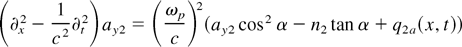
In second order we find from Eqs. (4)
where the source terms are quadratic in the first-order solution (9)
and are given by
The wave equation for the photon amplitude
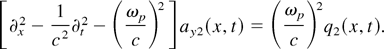
ay2 can be brought into the form
A complete expression for the source function
q2(x, t) was derived by Lichters
(1997). Here we collect only the two plasmon
terms of the form q2(x, t) =
q0 cos(ωT t
− kT x). For the amplitude
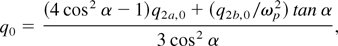
q0 we find after some algebra
with q2a,0 =
0.39φ02 and
q2b,0 =
−0.066ωp2φ02,
which are the corresponding amplitudes of the two source terms in Eq.
(19), evaluated for α = 55°, kp
c/ωp ≈ 1,
kT /kp
≈ 2.4, ωT /ωp
≈ 1.15. With these values, we obtain q0 ≈
0.022φ02 ≈ 2 ×
10−3, taking the estimate φ0 =
(k0
/kT)Ex0
/E0 ≈ 0.1 from Figure
9.
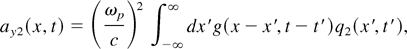
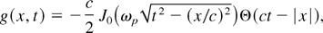
The solution of Eq. (20) is then obtained in the general form
using the Green function of the Klein–Gordon operator
where J0 denotes the Bessel function of first
kind. In the present case, we find the amplitude of the right-going
light wave at the right surface in the form
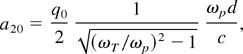
where d is the thickness of the foil. For d =
λ, we find ωp dc ≈ 25 and
a20 ≈ 5 × 10⁻³. Here we
neglect effects of reflection and refraction at the boundaries, which
are of order unity, and estimate the emission power at
ωT as a202 ≈
2 × 10⁻⁵. This is in reasonable agreement with
the value a202 ≈
10−5, obtained from the simulated
2ωp peak shown in Figure
12.
6. CONCLUSIONS
We conclude that ultrashort high-intensity laser pulses offer new
possibilities to generate high-amplitude plasma waves and to study
their interactions and decay into photons. The excitation of these
waves is mediated by bunches of relativistic electrons (jets)
accelerated by the laser light at the surface of a thin, overdense
plasma layer and shot into the layer periodically with the laser
frequency. The layer then starts to emit radiation at multiples of the
plasma frequency. So far, this radiation has not been observed, but
should be detractable with the intense few-cycle laser pulses now under
development. The physical mechanism is analogous to the generation of
solar type III radiation in the solar corona, and detection in laser
experiments may provide new possibilities to study the astrophysical
phenomenon in the laboratory.
The central result of this article is that this emission sets in only
after counterpropagating plasma waves have been created. Those
propagating opposite to the laser direction are driven by electron jets
that have been reflected by strong space charge fields building up at
the rear surface. In this article, we have studied the electron
dynamics by 1D PIC simulation and have recovered the main feature of
emission at plasma harmonics also analytically, solving the cold plasma
equations in second-order perturbation theory.
A major limitation of the present work is the restriction to
one-dimensional geometry, ignoring the fact that 2D and 3D effects
like, for example, crater formation (Pukhov &
Meyer-ter-Vehn, 1997) and current filamentation (Honda et al., 2000) can play a significant
role in relativistic laser plasma interaction. Nevertheless, we believe
that the present results give a correct description, at least
qualitatively, for configurations in which the focal diameter is much
larger than the layer thickness (thin layers) and ultrashort pulse
durations of only a few laser cycles during which hole-boring effects
can still be neglected. In view of the recent advances in generating
few-cycle laser pulses at ultrahigh intensities (Brabec & Krausz, 2000), one may expect that
experimental studies will become possible in the near future. For the
laser intensities of the order of 1018 W/cm2
considered here, thin low-Z target layers will turn into dense
plasma within the first laser cycle so that experiments may start from
solid material.
The present results also indicate that the configuration of a single
beam obliquely incident on a thin layer considered here may not be the
best possible for generating the radiation at plasma harmonics. Making
use of two laser beams incident from different directions and other
target geometries, one may succeed in creating plasmons propagating at
angles optimal for two-plasmon decay. Investigations of such options
require at least 2D simulation. It is hoped that the present results
will stimulate such work.
ACKNOWLEDGMENTS
Inspiring discussions with Harald Lesch and his group at Sternwarte
München on the astrophysical context of this work are gratefully
acknowledged. This work was supported by Deutsche
Forschungsgemeinschaft under contract Me444.