2. DOA ESTIMATION PRINCIPLE

The DOA represents the signal direction from the satellite to the user platform. It is a unit vector. Assuming a pair of antennas is fixed to the rigid platform, the SD between two antennas is equal to the baseline projection onto the DOA direction.

(1)$$\matrix{\eqalign{& {\Delta \rho _{ij}^m = {\bf g}_{ij}^T {\bf x}^m + c\Delta t_{ij} + \Delta l_b + \Delta \varepsilon _\rho} \cr & {\Delta \phi _{ij}^m = {\bf g}_{ij}^T {\bf x}^m + c\Delta t_{ij} + \Delta l_b + \lambda \Delta N_{ij}^m + \Delta \varepsilon _\phi} \cr}} $$

where x^m=(x^m, y^m, z^m)^T is the DOA vector for the mth satellite, Δρ _ij^m and Δφ _ij^m denote the SD pseudorange and carrier phase measurements between the reference antenna j and the auxiliary antenna i, g_ij=(g _ijx,g_ijy,g_ijz)^T is the antenna baseline, λ is the carrier wavelength, and ΔN _ij^m is the unknown integer ambiguity. It is well known that after single differencing between antennas over a short baseline, the spatially correlated orbital, tropospheric and ionospheric errors will significantly cancel, and the errors from the same source, like the satellite clock error, can also be eliminated. However, SD does not eliminate the receiver clock error cΔt _ij and the line bias Δl _b due to different receiver time tags and different cable lengths from two antennas to receivers. If double differences (DD) between two antennas and two satellites are constructed, cΔt _ij and Δl _b can also be cancelled out. However, DD cannot be used for DOA estimation, as it will result in the DOA differences between satellites, not the DOA itself. The combined effect of cΔt _ij and Δl _b can either be pre-calibrated or removed using a low pass filter, leaving only the receiver noise and multipath lumped together into Δε _ρ,Δε _φ.

The vectors x^m and g_ij can be expressed in either the body fixed coordinate or the local level coordinate such as the north-east-up frame as long as they are both in the same coordinate system. In the traditional GNSS model, both vectors are expressed in the local level coordinate system. The DOA can be coarsely calculated using the satellite ephemeris and pseudoranges, while the antenna baseline is unknown and can be precisely estimated when there are more than four satellites in view. In this case, Equation (1), after the removal of biases, can be extended to M (M≥4) satellites for a single baseline model:

(2)$$\matrix{\eqalign{& {\Delta {\bf P}_{ij} = {\bf g}_{ij}^T {\bf X} + \Delta {\bf \varepsilon} _{{\bf P}_{ij}}} \cr & {\Delta {\bf \Phi} _{ij} = {\bf g}_{ij}^T {\bf X} + \lambda \Delta {\bf N}_{ij} + \Delta {\bf \varepsilon} _{{\bf \Phi} _{ij}}} \cr}{\rm\hskip -3pt,\ subject\ to}\ \left\| {{\bf g}_{ij}} \right\|{\rm = L}} $$

where DOAs are in matrix X=[x¹,x² …, x^M], SD pseudorange and carrier phase observables are imbedded in ΔP_ij=[Δρ _ij¹, Δρ _ij² …, Δρ _ij^M]^T and ΔΦ_ij=[Δφ _ij¹, Δφ _ij² …, Δφ _ij^M]^T, and ΔN_ij includes M integers ΔN_ij=[ΔN _ij¹, ΔN _ij² …, ΔN _ij^M]^T. The antenna baseline g_ij in local level coordinates will be estimated. The baseline length is treated as a constraint to increase the reliability of ambiguity resolution in Teunissen (Reference Teunissen2006).

Alternately, both x^m and g_ij in Equation (1) can be expressed in the body fixed frame. Since antennas are rigidly fixed on the platform, the baseline coordinates are known in the body fixed frame while the DOA vector is now unknown. The model for the mth satellite and n antenna baselines is:

(3)$$\matrix{\eqalign{& {\Delta {\bf P}^m = {\bf Gx}^m + \Delta {\bf \varepsilon} _{{\bf P}^m}} \cr & {\Delta {\bf \Phi} ^m = {\bf Gx}^m + \lambda \Delta {\bf N}^m + \Delta {\bf \varepsilon} _{{\bf \Phi} ^m}} \cr} {\rm\hskip -3pt,\ subject\ to} \left\| {{\bf x}^m} \right\|{\rm = 1}} $$

where G=[g_1j^T; g_2j^T …; g_nj^T] is the baseline coordinate matrix for n baselines, SD pseudorange and carrier phase observables are between the auxiliary antennas and the reference antenna for the mth satellite, which are denoted as ΔP^m=[Δρ _1j^m, Δρ _2j^m …, Δρ _nj^m]^T and ΔΦ^m=[Δφ _1j^m, Δφ _2j^m …, Δφ _nj^m]^T. Here, ΔN^mincludes n integers ΔN^m=[ΔN _1j^m, ΔN _2j^m …, ΔN _nj^m]^T. The number of unknowns, including the DOA vector and ambiguities, is n+3, while the number of measurements is 2n. To solve the equation and also guarantee the G matrix has full column rank, this model imposes two requirements on the antennas: firstly, there must be at least three baselines (four antennas), and secondly, the array geometry must be non-planar.

Although Equation (2) and (3) are both SD models, Equation (3) shows two advantages over Equation (2). Firstly, the design matrix in Equation (3) is the antenna baseline matrix G, which has constant elements in the body fixed frame as long as they are fixed on the rigid platform, while the design matrix in Equation (2) is the LOS matrix X, which changes over time as the satellites and/or platform move in the local level frame. Since the design matrix needs to be decomposed for the integer ambiguity search, the decomposition of G is only performed once while the decomposition of X has to be repeated every epoch until the resolved ambiguities are validated (Sutton, Reference Sutton2002). Thus, this model has less computational load.

In addition, Equation (3) is performed using only the mth satellite. Other DOAs for other satellites can be estimated separately. Therefore, the model works independently of the number of GNSS satellites, which makes it ideal for working under conditions of low satellite visibility, such as in urban areas with signal blockage from high buildings, or for spacecraft in high earth orbit where it is difficult to receive sufficient GNSS signals. A special application is the relative navigation system in a two-spacecraft formation mission called PRISMA (Lestarquit et al., Reference Lestarquit, Harr and Trommer2006). To demonstrate the relative navigation capability in high earth orbit without visibility of GNSS satellites, GNSS-like signals are locally transmitted via an inter-satellite link from one spacecraft to the other. In this case, there is only one signal source, and multiple antennas have to be used for the signal reception in order to estimate the relative orientations and also to assist the determination of inter-satellite distance (Lestarquit et al., Reference Lestarquit, Harr and Trommer2006). Additional future space missions propose to use similar systems, e.g., the PROBA-3 mission (Garreau et al., Reference Garreau, Gantois and Cropp2010).

3. SINGLE DIFFERENCE WITH A COMMON CLOCK

Before resolving integer ambiguities, the receiver clock error and the line bias have to be calibrated and removed from the model.

To eliminate the receiver clock error, the same clock needs to be used. This requirement initiates two possible arrangements: firstly, a single receiver with connections to multiple antennas using a single internal clock; or secondly, multiple receivers driven by a common external clock.

In the first arrangement, the receiver clock error can be completely eliminated as the observations on two antennas come from two different channels in a single receiver. They share the same initial clock bias and also have the same clock drift over time. However, there are not many receivers available in the market with multiple antenna connections.

This paper uses the second arrangement, that is, to drive several receivers with an external common clock. This arrangement only assures that the clock drift over time is identical, while the initial biases for each receiver are likely to be different (Keong, Reference Keong1999). The reason is that the phase measurements are integrations of the phase rate. The common clock can only guarantee that the integrals are implemented in the same time slice, but the initial phases are different in different receivers. Therefore, SD with a common clock does not eliminate the clock error completely, but leaves a constant non-zero initial bias.

The line bias is due to the different cable lengths from two antennas to receivers, which is also constant over time. Given the fact that both of them are constant, the combined bias can then be estimated in a low pass filter (Keong, Reference Keong1999):

(4)$$est_i = \displaystyle{{i - 1} \over i}est_{i - 1} + \displaystyle{1 \over i}res_i $$

where est is the estimated bias, res is defined as a residual bias and i is the epoch counter. The estimated bias will be fed back to the system at the subsequent epoch.

For the code observable, the residual bias is:

(5)$$res_{i,\rho} = \Delta \rho _i - \Delta r_{i - 1} $$

where Δr _i−1 is the estimation of the SD range in the last epoch after the feedback of the estimated bias.

For the phase observable, the residual bias may contain several wavelengths, which will be absorbed by the ΔN term, leaving a fractional part with magnitude typically at the centimetre level. This fractional part of residual bias is:

(6)$$\eqalign{& res_{i,\phi} = \Delta \phi _i - \Delta r_{i - 1} - \lambda \Delta N_i \cr & \Delta N_i = \left[ {\displaystyle{{\Delta \phi _i - \Delta r_{i - 1}} \over \lambda}} \right]} $$

The bias estimate does not need to be as accurate as the DOA estimation, since the ambiguity resolution method in the following section has a certain tolerance to bias (Teunissen et al., Reference Teunissen, Joosten and Tiberius2000).

4. INTEGER AMBIGUITY RESOLUTION: LAMBDA

After removing the constant bias and also omitting the superscript m in Equation (3) to generalize the model for one satellite, the dual-frequency equation can be written as,

(7)$$\left[ {\matrix{ {\Delta {\bf P}} \cr {\Delta {\bf \Phi} _{\,f1}} \cr {\Delta {\bf \Phi} _{\,f2}} \cr}} \right] = \left[ {\matrix{ {\bf G} & {} & {} \cr {\bf G} & {\lambda _1 {\bf I}_n} & {} \cr {\bf G} & {} & {\lambda _2 {\bf I}_n} \cr}} \right]\left[ {\matrix{ {\bf x} \cr {\Delta {\bf N}_{\,f1}} \cr {\Delta {\bf N}_{\,f2}} \cr}} \right] + \Delta {\bf \varepsilon}, {\rm subject\,to} \left\| {\bf x} \right\|{\rm = 1} $$

which can be further grouped into the following model:

(8)$$\eqalign{& {{E({\bf y}) = {\bf Bx} + {\bf Aa} = (\matrix{ {\bf B\quad A} \cr} )\left( {\matrix{ {\bf x} \cr {\bf a} \cr}} \right),{\rm} {\bf x} \in {\opf R}^{3}, {\rm} {\bf a} \in {\opf Z}^{2n} {\rm,} \left\| {\bf x} \right\|{\rm = 1}}} \cr & D({\bf y}) = {\bf Q}_{{\bf yy}}} $$

with

(9)$$\eqalign{& {{\bf y} = \left[ {\Delta {\bf P}\ {\rm} \Delta {\bf \Phi} _{\,f1} {\rm}\ \Delta {\bf \Phi} _{\,f2}} \right]^T} \cr & {\bf B} = \left[ {\matrix{ 1 & 1 & 1 \cr}} \right]^T \otimes {\bf G} \cr & {\bf A} = \left[ {\matrix{ {\bf 0} & {diag(\lambda _1, \lambda _2 )} \cr}} \right]^T \otimes {\bf I}_n \cr & {\bf a} = \left[ {\matrix{ {\Delta {\bf N}_{\,f1}} & {\Delta {\bf N}_{\,f2}} \cr}} \right]} $$

where E() and D() are the mathematical expectation and dispersion operators, and ⊗ is the Kronecker product. The precision of observations is described by the covariance matrix Q_yy.

Disregarding the unitary constraint of x in Model (8) and only applying the integer constraints for ambiguities, the standard LAMBDA method can be used (Teunissen, Reference Teunissen1995). The first step in LAMBDA is to obtain the so-called float solutions using a standard least-squares adjustment. Real-valued estimates of the DOA vector and ambiguities are available, together with their associated covariance matrix:

(10)$$\left[ {\matrix{ {{\bf \hat x}} \cr {{\bf \hat a}} \cr}} \right]{\rm,} \left[ {\matrix{ {{\bf Q}_{{\bf \hat x\hat x}}} & {{\bf Q}_{{\bf \hat x\hat a}}} \cr {{\bf Q}_{{\bf \hat a\hat x}}} & {{\bf Q}_{{\bf \hat a\hat a}}} \cr}} \right] = \left[ {\matrix{ {{\bf B}^T {\bf Q}_{{\bf yy}}^{ - 1} {\bf B}} & {{\bf B}^T {\bf Q}_{{\bf yy}}^{ - 1} {\bf A}} \cr {{\bf A}^T {\bf Q}_{{\bf yy}}^{ - 1} {\bf B}} & {{\bf A}^T {\bf Q}_{{\bf yy}}^{ - 1} {\bf A}} \cr}} \right]^{ - 1} $$

The next step is to map all the float ambiguities â to the corresponding integer values ${\bf \breve {a}} $ through a search process. A search is implemented to minimize the ambiguity objective function in the Integer Least Squares (ILS):

(11)$${\bf \breve {a}} = \mathop {\min} \limits_{{\bf a} \in {\opf Z}^{2n}} \left\| {{\bf \hat a} - {\bf a}} \right\|_{{\bf Q}_{{\bf \hat a\hat a}}} ^2 $$

where $\left\|. \right\|_{{\bf Q}_{{\bf \hat a\hat a}}} ^2 = (.)^T {\bf Q}_{{\bf \hat a\hat a}}^{ - 1} (.)$. Using the Cholesky decomposition for Q_ââ⁻¹, the search can be efficiently implemented in the sequential conditional adjustment (Jonge and Tiberius, Reference Jonge and Tiberius1996).

Once the integer ambiguities are correctly sought, they can be used to estimate the final parameters of interest with high precision in the final and third step of LAMBDA.

5. BOUNDING AMBIGUITY SEARCH WITH THE CONSTRAINT

Two types of constraints should be clarified at this moment: the integer constraints on the ambiguities, and the unit length constraint on the DOA vector ||x||=1. They play a distinct role in the estimation. The presence of the integer ambiguities enables precise DOA estimation, whereas the presence of the unit length constraint can be embedded in the ambiguity search space and will enable high ambiguity resolution success rates and therefore reliable DOA estimation.

The DOA length is written as

(12)$$\left\| {\bf x} \right\|^2 = {\bf x}^T {\bf x} = 1$$

If ambiguities are divided into two subsets, the primary subset with three ambiguities and the second subset with the rest of ambiguities, the DOA vector can be calculated using only the primary subset.

(13)$${\bf a} = \left[ {\matrix{ {{\bf a}_{\bf p}} & {{\bf a}_{\bf s}} \cr}} \right]^T, {\rm} {\bf a}_{\bf p} \in {\opf Z}^3, {\rm} {\bf a}_{\bf s} \in {\opf Z}^{2n - 3} $$

(14)$${\bf \breve {x}} ({\bf a}_{\bf p} ) = {\bf G}_{\bf p}^{ - 1} (\Delta {\bf \Phi} _{\bf p} - {\bf A}_{\bf p} {\bf a}_{\bf p} )$$

where G_p corresponds to the first three rows in the G matrix and represents three of the antenna baselines, A_p=λ ₁I₃(or λ ₂I₃) contains the wavelengths of the carrier frequencies. Only three ambiguities are used to assure G_p is a full rank matrix and invertible.

Substituting Equation (14) into (12) and also replacing the unit length by lower and upper boundaries (1−δl)²and (1+δl)², the quadratic equality constraint becomes a set of inequality boundaries.

(15)$$(1 - \delta l)^2 \le (\Delta {\bf \Phi} _{\bf p} - {\bf A}_{\bf p} {\bf a}_{\bf p} )^T {\bf G}_{\bf p}^{ - T} {\bf G}_{\bf p}^{ - 1} (\Delta {\bf \Phi} _{\bf p} - {\bf A}_{\bf p} {\bf a}_{\bf p} ) \le (1 + \delta l)^2 $$

This can be translated to the same form as $\left\| {{\bf \hat a} - {\bf a}} \right\|_{{\bf Q}_{{\bf \hat a\hat a}}} ^2 \le \chi ^2 $,

(16)$$\Omega _{{\bf a}_{\bf p}, - \delta l} {\rm} = \left\{ {{\bf a}_{\bf p} \in {\opf Z}^3 \left| {\left\| {\Delta {\bf \Phi} _{\bf p} - {\bf A}_{\bf p} {\bf a}_{\bf p}} \right\|_{{\bf G}_{\bf p}^{} {\bf G}_{\bf p}^T} ^2 \le (1 - \delta l)_{}^2} \right.} \right\}$$

(17)$$\Omega _{{\bf a}_{\bf p}, + \delta l} {\rm} = \left\{ {{\bf a}_{\bf p} \in {\opf Z}^3 \left| {\left\| {\Delta {\bf \Phi} _{\bf p} - {\bf A}_{\bf p} {\bf a}_{\bf p}} \right\|_{{\bf G}_{\bf p}^{} {\bf G}_{\bf p}^T} ^2 \le (1 + \delta l)_{}^2} \right.} \right\}$$

The integer candidates bounded by (1−δl)² and (1+δl)²are collected in the set $\Omega _{{\bf a}_{\bf p}, - \delta l} $ and $\Omega _{{\bf a}_{\bf p}, + \delta l} $, respectively. Only the candidates in set $\Omega _{{\bf a}_{\bf p}, + \delta l} $ without $\Omega _{{\bf a}_{\bf p}, - \delta l} $ will be accepted for the further search of the minimizer. To solve the inequalities, the sequential conditional adjustment is used. By LDL^T-decomposition of the matrix G_p^−TG_p⁻¹ using the lower triangular matrix L and the diagonal matrix D, the quadratic inequality, e.g., in Equation (16) can be written as

(18)$$\sum\limits_{i = 1}^3 {d_i \left[ {(\lambda a_i - \Delta \Phi _{\,pi} ) + \sum\limits_{\,j = 1}^{i - 1} {l_{ij} (\lambda a_j - \Delta \Phi _{\,pj} )}} \right]} ^2 \le \left( {1 - \delta l} \right)^2 $$

where d _i and l _ij are the diagonal elements in D and the lower triangular elements in L, respectively. The sequential conditional adjustment is performed by rewriting Equation (18) in three sequential intervals for searching each of the ambiguities.

(19)$$\eqalign{& { d_1 (\lambda a_{\,p1} - \Delta \Phi _{\,p1} )^2 \le (l - \delta l)^2} \cr & d_2 (\lambda a_{\,p2} - \Delta \Phi _{\,p2} \left| {_{\,p1}} \right.)^2 \le (l - \delta l)^2 - d_1 (\lambda a_{\,p1} - \Delta \Phi _{\,p1} )^2 \cr & d_3 (\lambda a_{\,p3} - \Delta \Phi _{\,p3} \left| {_{\,p1,p2}} \right.)^2 \le (l - \delta l)^2 - d_1 (\lambda a_{\,p1} - \Delta \Phi _{\,p1} )^2 - d_2 (\lambda a_{\,p2} - \Delta \Phi _{\,p2} \left| {_{\,p1}} \right.)^2} $$

where the conditional estimates for ΔΦ_p2 and ΔΦ_p3 are defined as ΔΦ_p2| _p1 and ΔΦ_p3| _p1,p2, which are conditioned on the previous estimated integers of a _p1 and a _p1, a _p2.

(20)$$\eqalign{& {\Delta \Phi _{\,p2} \left| {_{\,p1}} \right. = \Delta \Phi _{\,p2} - l_{21} (\lambda a_{\,p1} - \Delta \Phi _{\,p1} )} \cr & \Delta \Phi _{\,p3} \left| {_{\,p1,p2}} \right. = \Delta \Phi _{\,p3} - l_{31} (\lambda a_{\,p1} - \Delta \Phi _{\,p1} ) - l_{32} (\lambda a_{\,p2} - \Delta \Phi _{\,p2} )} $$

Similar expressions can be written to the upper bound of (1+δl)².

The search procedure is then implemented following Equation (21) to (25),

(21)$${\opf C}^3 = \Omega _{{\bf a}_{\bf p}, + \delta l} \backslash \Omega _{{\bf a}_{\bf p}, - \delta l} $$

(22)$$\Omega _{{\bf a}_{\bf p}} = \left\{ {{\bf a}_{\bf p} \in {\opf C}^3 \cap {\opf Z}^3 \left| {\left\| {{\bf \hat a}_{\bf p} - {\bf a}_{\bf p}} \right\|_{{\bf Q}_{{\bf \hat a}_{\bf p} {\bf \hat a}_{\bf p}}} ^2 \le \chi ^2} \right.} \right\}$$

(23)$$\Omega _{{\bf a}_{\bf s} \left| {{\bf a}_{\bf p}} \right.} = \left\{ {{\bf a}_{\bf s} \in {\opf Z}^{2n - 3} \left| {\matrix{ {\left\| {{\bf \hat a}_{\bf s} - {\bf a}_{\bf s}} \right\|_{{\bf Q}_{{\bf \hat a}_{\bf s} {\bf \hat a}_{\bf s}}} ^2 \le \chi _{}^2} \cr {{\rm conditioned\ on}\ {\bf a}_{\bf p} \in \Omega _{{\bf a}_{\bf p}}} \cr}} \right.} \right\}$$

(24)$${\opf C}^{2n} = \Omega _{{\bf a}_{\bf p}} \cup \Omega _{{\bf a}_{\bf s} \left| {{\bf a}_{\bf p}} \right.} $$

(25)$${\bf \breve {a}} {\rm} = \mathop {\min} \limits_{{\bf a} \in {\opf C}^{2n} \cap {\opf Z}^{2n}} \left\| {{\bf \hat a} - {\bf a}} \right\|_{{\bf Q}_{{\bf \hat a\hat a}}} ^2 $$

Equation (21) means that an integer set ℂ³ for the first three ambiguities only accepts the candidates in set $\Omega _{{\bf a}_{\bf p}, + \delta l} $ without $\Omega _{{\bf a}_{\bf p}, - \delta l} $. The standard quadratic form $\left\| {{\bf \hat a}_{\bf p} - {\bf a}_{\bf p}} \right\|_{{\bf Q}_{{\bf \hat a}_{\bf p} {\bf \hat a}_{\bf p}}} ^2 $ can still apply, but now over a smaller region ℂ³⊂ℤ³, instead of over the complete space ℤ³. Therefore, the constraint is fulfilled in the way that this smaller region ℂ³ can exclude some wrong candidates in the early stage of the search, leading to the conditional search space in Equation (23) for the second subset of ambiguities that is also smaller than the unconstrained version. To this end, minimizing the objective function of Equation (25) will be intrinsically different to the minimization of the standard unconstrained objective function of Equation (11) because the minimizer is searched in a smaller and more precise integer region ℂ²ⁿ.

After ambiguities are fixed with the unit length constraint, the final DOA vector can be corrected using the complete set of ambiguities:

(26)$${\bf \breve {x}} ({\bf \breve {a}} ) = {\bf \hat x} - {\bf Q}_{{\bf \hat b\hat a}} {\bf Q}_{{\bf \hat a\hat a}}^{ - 1} ({\bf \hat a} - {\bf \breve {a}} )$$

Its covariance matrix is

(27)$${\bf Q}_{{\bf \breve {x}} ({\bf \breve {a}} ){\bf \breve {x}} ({\bf \breve {a}} )} = \displaystyle{{\sigma _\phi ^2} \over 2}({\bf G}^T ({\bf WW}^T )^{ - 1} {\bf G})^{ - 1} $$

where W represents the SD operator and is equal to [I_n,− e_n] to account for n baselines, e_n is the unit column matrix, and the denominator “2” means the number of frequencies is two.

The strategy of utilizing the constraint can also be explained by Figure 1, which depicts the float DOA distribution and the unconstrained fixed DOA distributions based on 10⁴ epochs of simulated estimates. The blue dots represent the float DOA distribution, which shows an elongated ellipse due to the correlations between its coordinates. The centre of the ellipse will be the correct DOA solution. The unconstrained fixed DOA distributions are shown as either red or yellow dots: red if the ambiguities are wrongly fixed, yellow if they are correctly fixed. These unconstrained solutions are obtained by only applying the minimization in the standard ILS as in the case of the original LAMBDA method. It is clear that, without the constraint, only a part of the resultant ILS minimizers can lead to the correctly fixed DOA in yellow, while a high percentage of the ILS minimizers cause the fixed DOA distributed to include non-physical locations shown in red. Therefore, the lower and upper circular boundary ring can play a dramatic role in excluding the wrong minimizers. It is easy to reject the wrong minimizers that lead to the DOA distribution far away from the boundary ring. However, it is difficult to exclude the ones that are wrong solutions but still make the resultant DOA drop into the boundary ring. Those minimizers are called false alarm minimizers. The width of the boundary ring determines the percentage of the false alarm minimizers, which needs to be adaptive to the quality of the model. Making the boundary ring too wide will increase the probability that wrong minimizers become false alarm minimizers, while making it too narrow risks missing the correct solution.

Figure 1. Two-dimensional float DOA distributions (blue) and the corresponding unconstrained fixed DOA (yellow or red). In (a), 69·2% of the 10⁴ solutions are correctly fixed (yellow), while 30·8% are wrongly fixed (red); In (b), the correctly and wrongly fixed solutions are 13·9% (yellow) and 86·1% (red), respectively. Lower and upper boundaries (black) show the ability to exclude the wrong solutions and remain the correct solutions.

Out of the 10⁴ float solutions, only 69·2% and 13·9%, respectively, in Figure 1 (a) and (b) are correctly fixed without the constraint. After constraining, the success rates increase to 99·2% and 39·2%, respectively, which are shown in Figure 2 (a) and (b) where the green dots represent the constrained fixed DOA results. It is clear that these constrained DOA vectors are scattered on the surface of the lower boundary sphere, indicating that the constraint is fulfilled in the ILS.

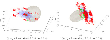
Figure 2. Three-dimensional float DOA distributions (blue) and unconstrained (red) and constrained (green) fixed DOA distributions. The constrained results are scattered on the surface of the lower boundary sphere. The upper boundary sphere is not depicted in the figure for clarity.

6. THRESHOLD

The width of the boundary ring, determined by the threshold δl, is critical for the constrained ambiguity search. Since the covariance matrix ${\bf Q}_{{\bf \breve {x}} ({\bf a}_{\bf p} ){\bf \breve {x}} ({\bf a}_{\bf p} )} $ governs the fixed DOA vector distribution, δl should then be calculated according to ${\bf Q}_{{\bf \breve {x}} ({\bf a}_{\bf p} ){\bf \breve {x}} ({\bf a}_{\bf p} )} $.

(28)$${\bf Q}_{{\bf \breve {x}} ({\bf a}_{\bf p} ){\bf \breve {x}} ({\bf a}_{\bf p} )} = {\bf G}_{\bf p}^{ - 1} {\bf Q}_{\Delta {\bf \Phi} _{\bf p} \Delta {\bf \Phi} _{\bf p}} ^{} {\bf G}_{\bf p}^{ - T} $$

where ${\bf Q}_{\Delta {\bf \Phi} _{\bf p} \Delta {\bf \Phi} _{\bf p}} ^{} = \sigma _\phi ^2 {\bf W}_{\bf p} {\bf W}_{\bf p}^T $ is the SD phase noise matrix and W_p is the SD operator for three baselines W_p=[I₃,− e₃]. This equation shows that ${\bf Q}_{{\bf \breve {x}} ({\bf a}_{\bf p} ){\bf \breve {x}} ({\bf a}_{\bf p} )} $ depends upon the measurement noise ${\bf Q}_{\Delta {\bf \Phi} _{\bf p} \Delta {\bf \Phi} _{\bf p}} ^{} $ and the way in which the noise is attenuated by the baseline matrix G_p. An appropriate boundary threshold δl can be obtained from the trace of the covariance matrix.

(29)$$\sigma _{\left\| {{\bf \breve {x}} ({\bf a}_{\bf p} )} \right\|}^{} = \sqrt {tr({\bf Q}_{{\bf \breve {x}} ({\bf a}_{\bf p} ){\bf \breve {x}} ({\bf a}_{\bf p} )} )} = \displaystyle{{\sigma _\phi ^{}} \over {\sqrt {tr({\bf G}_{\bf p}^T ({\bf W}_{\bf p} {\bf W}_{\bf p}^T )^{ - 1} {\bf G}_{\bf p}^{} )}}} $$

where tr() denotes trace.

The constraint bounding is essentially a hypothesis testing procedure using the length of the conditional DOA vector as test statistic. If there is no correlation between the coordinates of the fixed DOA vector, the DOA length is Gaussian distributed and the threshold δl can then to be chosen to $3\sigma _{\left\| {{\bf \breve {x}} ({\bf a}_{\bf p} )} \right\|}^{} $ to assure that the correct solution will pass the test at a confidence as high as 99·7%. However, 3-sigma boundary ring may still include too many wrong solutions. Figure 3 depicts the DOA distributions bounded by both 1-sigma and 3-sigma rings. Variable phase noise and baseline geometries are assumed in Figure 3 (a–c), which leads to different distribution shapes and sizes. Compared to (a), (b) is more noisy while (c) has a “bad” baseline geometry with smaller angular separations. Boundary rings thus show different widths in different cases. However, it is clear that out of 10⁴ epochs of estimates, the correctly fixed solutions all completely fall into the 3-sigma and partly fall into the 1-sigma boundary ring in all cases. On one hand, this verifies the statement that δl can be determined according to ${\bf Q}_{{\bf \breve {x}} ({\bf a}_{\bf p} ){\bf \breve {x}} ({\bf a}_{\bf p} )} $. On the other hand, a compromise between maximally including the correct solution and rejecting the wrong solutions requires δl to be chosen between 1-sigma and 3-sigma.

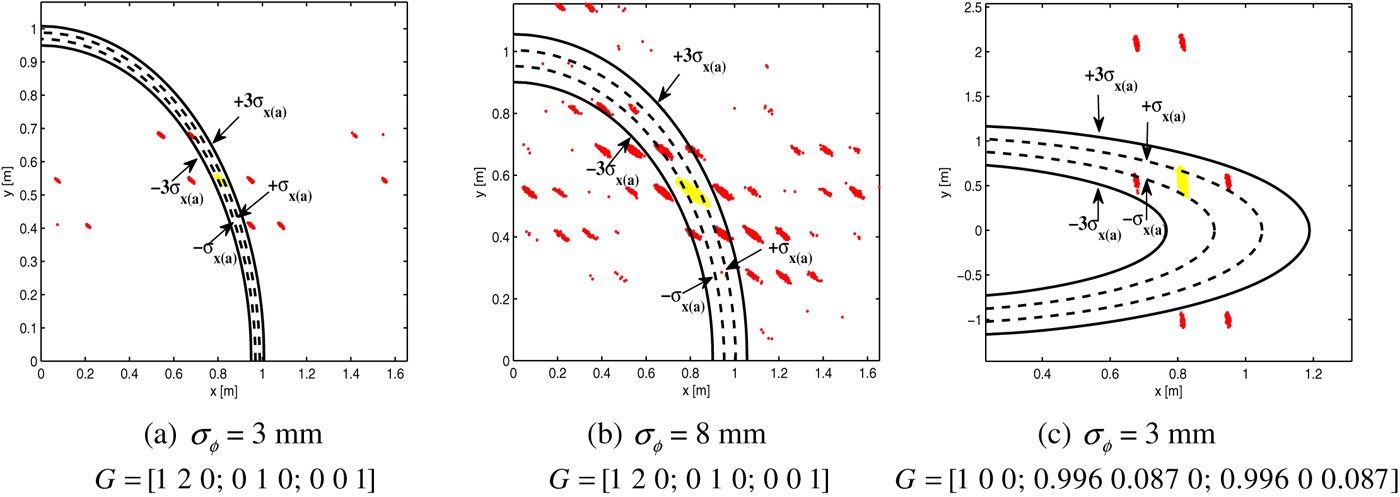
Figure 3. Two-dimensional unconstrained fixed solutions (yellow or red): yellow if ambiguities are correctly fixed, red if they are wrongly fixed. The 3-sigma boundary ring (black) is relatively wide to exclude the wrong solutions, while the 1-sigma boundary ring (black dash) is rather narrow and risks missing the correct solution.

The threshold δl is assumed k times $\sigma _{\left\| {{\bf \breve {x}} ({\bf a}_{\bf p} )} \right\|}^{} $. Simulations are performed with k ranging from 0·5 to 3 for different configurations given different code and phase noise, variable baseline numbers and geometries, dual or triple frequencies. If any of these parameters change, the quality of the model will change. The bootstrapping lower bound success rate can serve as an indicator to characterize the quality of the model at different configurations (Verhagen, Reference Verhagen2005). Once more than three antenna baselines or more than one frequency are involved, the number of ambiguities will be larger than three. According to Equation (30), the criteria of choosing three of them as the primary subset ambiguities are: firstly, a_p are on the frequency (L1 or L2) which provides smaller phase noise and secondly, a_p are for those three baselines that lead to larger values of the entries in G_p^T(W_pW_p^T)⁻¹G_p. It can be achieved by choosing three baselines with larger lengths or better arrangements of their relative positions.

Figure 4 depicts four configurations that result in the bootstrapping success rate ranging from 25% to 95%. For all ranges of k, the empirical success rate is calculated which is defined as the percentage of occurrences where the computed integer solution is equal to the true integer vector. Being independent of δl, the empirical success rates for the original LAMBDA are identical for all k, although a small oscillation exists from the use of different sets of random data for different k. With the constraint, the largest empirical success rate then occurs in (a) and (c) when k is close to 1·5, while in (b) and (d), the largest success rate keeps approaching to 1 when k is larger than 1·5. The ultimate choice of k is 1·75 for all scenarios so that a good bounding performance can be guaranteed for high quality models and only a small loss of success rate has to be sacrificed for low quality models. The rule-of-thumb for δl is thus

(30)$$\delta l = 1{\cdot}75\displaystyle{{\sigma _\phi ^{}} \over {\sqrt {tr({\bf G}_{\bf p}^T ({\bf W}_{\bf p} {\bf W}_{\bf p}^T )^{ - 1} {\bf G}_{\bf p}^{} )}}} $$

Figure 4. The effect of δl.

7. FIELD TEST

To validate the algorithm, a field test was implemented on the roof of a building at the University of Calgary. As shown in Figure 5, five Novatel 702GG antennas, five Novatel OEMV dual-frequency receivers and an external oven-controlled crystal oscillator (OCXO) at 10 MHz were used. The OCXO signals were sent through a splitter to feed the primary and all other secondary receivers. The 1PPS output signal from the primary receiver was also physically fed to other secondary receivers in order to synchronize clocks. Antennas were arranged at different heights and variable locations. Their precise coordinates were carefully calibrated using the DD solution. The east-north-up frame is used as the body fixed frame in this field test. Antenna 3 was assumed as the reference antenna. Baseline coordinates of other antennas with respect to antenna 3 were

(31)$${\bf G} = \left[ {\matrix{ {{\bf g}_{13}} \cr {{\bf g}_{23}} \cr {{\bf g}_{43}} \cr {{\bf g}_{53}} \cr}} \right] = \left[ {\matrix{ { - 0{\cdot}709} & { - 1{\cdot}124} & {0{\cdot}361} \cr {0{\cdot}394} & { - 1{\cdot}066} & { - 0{\cdot}358} \cr {0{\cdot}992} & {0{\cdot}057} & { - 0{\cdot}137} \cr {1{\cdot}147} & { - 1{\cdot}244} & { - 0{\cdot}168} \cr}} \right]$$

Figure 5. Field test set-up.

Figure 6. Sky plot of the field test.

The heights of antennas 2 and 5 were lower than a wall located on the West side of the building, which might introduce multipath when the satellites are at low elevations to the West. In these circumstances, signal interruptions or corruptions are likely to happen and manifest themselves in cycle slips or losses of lock. Since the algorithm aims to a single-epoch solution, cycle slips and losses of lock would not affect the algorithm as in a filter. However, their occurrences will reduce the number of usable antennas in the epoch that is used for the solution. This paper will demonstrate that as long as four of the antennas have uncorrupted observables, cycle slips and losses of lock can be tolerated on the other antennas. In addition, cycle slips and losses of lock may interrupt the constant bias estimation in the low pass filter. Whether the bias will change was also examined in the field test.

Cycle slips were detected by high-order phase differencing (Dai, Reference Dai2012) which represents a sudden integer jump in the observations. Loss of lock is defined as the moment when the phase tracking loop is broken and the phase observable shows zero in the RINEX file. Taking PRN 9 for example, Table 1 shows the worst data quality was on antenna 2, which might be caused by multipath. The losses of lock on the L2 frequency are more frequent than on L1 as the signal strength is 3 dB lower on L2.

Table 1. Statistics of cycle slips and losses of lock for Satellite PRN 9 moving from 20° elevation to 4° elevation.

7.1. Bias Estimation

The field test was implemented with five OEMV receivers driven by an external clock. This leaves constant biases over time in SD code and phase observables, which revealed the differences in the cable lengths from antennas to receivers, as well as the differences in the initial phase biases given by different receivers.

Figures 7 and 8 depict the code and phase bias estimation for PRN 9. Generally, they all converged to a steady state after being processed in the low pass filter. Code biases are at metre level, while phase biases have a centimetre magnitude after their integer parts are absorbed by the ambiguities, leaving only the fractional parts. The theoretical maximum phase bias should be therefore no larger than half of the wavelength.

Figure 7. SD code bias estimate for PRN 9.

Figure 8. SD phase bias estimate for PRN 9.

The steady state, however, could be interrupted by cycle slips or losses of lock, e.g., SD on antenna 2 & 3 (yellow) and antenna 5 & 3 (green) for L2 frequency in Figure 8. Biases are re-estimated once there is a cycle slip or loss of lock in the algorithm. However, after re-estimation, the estimated phase bias still converges to the steady state that is at the same level as the previous bias before disturbance. This means cycle slips and losses of lock do not change the values of the fractional part of the initial phase biases. The consistency is not perfect because the number of the observables between two sequential disturbances is insufficient for the low pass filter to reach the ultimate steady state. The phase bias re-estimation for the antennas 2 & 3 on L1 frequency (dark green) is an exception because the bias is close to half of the wavelength. After the integer part is absorbed by the integer ambiguity, the remaining fractional part changes its sign from −0·5 cycle to +0·5 cycle. The true ambiguity is accordingly changed by a cycle after re-estimation.

Once the biases are calibrated and fed back to the SD measurements, zero-mean residuals are obtained, as depicted in Figures 9 and 10. The remaining 2-m and 2-cm fluctuations on the SD code and phase residuals are due to multipath that cannot be cancelled out by differencing. The SD noise value is amplified by a factor of $\sqrt 2 $ than the noise of the undifferenced observables. Therefore, the standard derivations for code and phase measurements for PRN 9 are 0·8 m and 8 mm, respectively, including the effects of multipath.

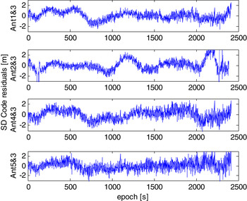
Figure 9. SD code residuals of PRN 9 after bias estimate feedback.

Figure 10. SD phase residuals of PRN 9 after bias estimate feedback.

7.2. IAR Performance and DOA Accuracy

After the bias removal, the integer ambiguity resolutions on single-epoch observations were implemented for each of the satellites separately. The results are presented in Table 2.

Table 2. Statistics of integer ambiguity resolution and DOA accuracy.

It is clear that ambiguities can be resolved with high success rate using only single epochs. By making use of the unit length constraint, the performance is dramatically improved. Referring to the field test set-up in Figure 5 and the sky plot in Figure 6, Satellite PRN 9, 29, 31 and 27 have elevations less than 20° in the direction of the wall. Their measurements are vulnerable to disturbances. The percentages of disturbances for these four satellites are 11·4%, 17·5%, 6·02% and 2·55%, respectively, out of the total epochs. The original LAMBDA method fails to resolve ambiguities when disturbances happen. However, the constrained LAMBDA can improve the performance by 9·33%, 16·49%, 1·72% and 2·55%, respectively, using only the remaining uncorrupted observables. This implies that the algorithm has tolerance to signal interruption or corruption as long as four antennas are remaining with uncorrupted observables.

For Satellite PRN 17 and 5 that face against the wall at low elevations, signal blockages may occur on antenna 2. In this circumstance, the success rates after constraining have been improved by up to 45% compared to the original LAMBDA method. For Satellite PRN 25 and 10 at the elevations between 25° and 45°, neither cycle slips nor losses of lock occur. The success rates are higher than 99%. For Satellite PRN 4, 2 and 12 at the elevations higher than 45°, both the original LAMBDA method and the LAMBDA with the constraint can reach 100% success rate using a single epoch. This means fast and reliable estimation is easy to achieve in open sky.

The last two columns show the DOA accuracy for each satellite. According to Equation (27), the DOA accuracy in x=(x,y,z)^T can reach a precision in accordance with the phase measurements after ambiguities are correctly fixed. They are transformed to elevation and azimuth angles in degrees. From Table 2, the elevation accuracy is around 1° in case of high occurrences of signal disturbances, while the accuracy improves to 0·1° as better quality signals are obtained. The azimuth accuracy is less than 0·3° for all the circumstances.

8. CONCLUSIONS AND RECOMMENDATIONS

This paper presents a method to estimate the GNSS signal directions of arrival based on carrier phase measurements. The integer cycle ambiguities have been quickly and reliably resolved by taking advantage of a constraint and using a non-planar antenna array with at least four elements. Having more than four elements provides redundancy for the ambiguity resolution as well as allowing tolerance of the signal interruption or corruption. The quadratic equality constraint has been translated to inequality boundaries so that the efficient sequential conditional adjustment can be performed. The standard ambiguity objective function is minimized, but in a reduced and precise search space. A rule-of-thumb for the search bounds was derived, providing insightful guidance on how to choose boundaries according to the noise level and antenna geometry.

A field test was implemented to demonstrate the proposed method. Antennas were connected to multiple receivers with a shared external clock. In this way, the common clock drift over time was cancelled out by differencing, leaving only a constant initial bias to be filtered in a low pass filter and fed back to the observables. An advanced receiver with multiple antenna connections is more suitable for this application as neither a dedicated external clock nor the calibration of initial clock bias is required. From field tests, high success rates were guaranteed and high DOA accuracy was obtained based on single-epoch single-satellite measurements.