II. THE D-RADAR ARCHITECTURE AND ITS TECHNOLOGICAL DEMONSTRATOR DANTE

The d-Radar [Reference Madia and Maestrini3–Reference Galati, Madia, Carta, Piracci, Franco and Quattrociocchi6] architecture has separate transmit and receive antennas based on conformal arrays [Reference Josefsson and Persson7–Reference Wirth10] on a conical surface (hence the terms bistatic and conformal), as shown in Fig. 1, where the transmitting (Tx) array is on the bottom and the receiving (Rx) array on the top. The arrays are composed by tilted columns, each one containing equidistant radiating or receiving elements, and a typical tilt angle of 15°.

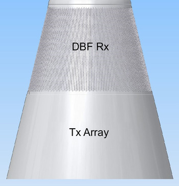
Fig. 1. The “bistatic” d-Radar antenna.

This concept is being field-tested by means of an X-band demonstrator called digital antenna evaluator ( DAntE ), operational by 2015; see Fig. 2.

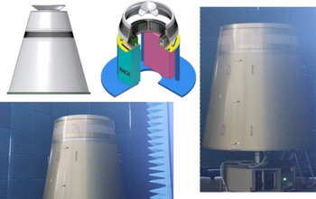
Fig. 2. The DAntE demonstrator and its installation in the SEASTEMA laboratories, Roma.

DAntE operates in a two-dimensional (2D) mode (i.e. without height measurement) with a conical receiving array whose columns have a reduced (eight only) number of elements each one. There are 200 columns (more precisely, 216 for the receiving array and 240 for the future bottom-installed transmitting array) and each one of them is connected to its own digital receiver. A physical unit called Q-pack groups four digital receivers, therefore there are over 50 Q-packs (i.e. 54 Q-packs for 216 receiving columns). The transmitting section is presently emulated by two independent antenna horns which can be aimed at different angles. A dedicated radar processor controls the DAntE operation.

Among the various topics being investigated with this demonstrator, there are the following, related to the receiving array, and aimed to check the capability of this conical, DBF array:

1. (i). Array pattern control (gain, side lobes reduction, synchronization in digital down conversion, etc.);

2. (ii). Multiple beam pointing (angular resolution, creation on nulls in defined directions, operation with multiple frequencies, etc.);

3. (iii). Data management (digital interfaces, data flow, data rate, etc.)

The programmed tests include:

1. 1. Array pattern: comparison between computed/simulated and measured patterns of conical arrays made up by a variable number of contiguous columns;

2. 2. Decoupling of receiving beams, with the transmitting beams:

   1. a) operating at a fixed frequency,

   2. b) operating at different frequencies,

   3. c) emitting orthogonal signals (generated by either deterministic or pseudo-random codes).

In fact, a relevant problem for this kind of radar architecture (but also present in more conventional phased array radars) is the coupling of the simultaneous beams in different operating conditions.

Among the results obtained with DAntE, there is the measured antenna pattern shown in Fig. 3.

Fig. 3. DAntE measured receiving antenna pattern at 9.5 GHz (the test antenna, representing the d-Radar operation as shown in Figs 4 and 5, was a subarray in a 107° sector, i.e. using 30% of the full number of columns).

Fig. 4. The electronic scan in azimuth.

Fig. 5. Different antenna configurations.

This concludes the description of DAntE: the remainder of this paper is fully dedicated to the d-Radar.

The key feature of d-Radar is the possibility to transmit and receive multiple simultaneous beams by partitioning of the Tx antenna and extensive usage of DBF as explained in the following, in order to implement a multifunction radar for both naval and ground-based applications, mainly aimed to point defense.

A subarray, defined by a group of adjacent columns from the Tx antenna, transmits on the selected, pertaining direction, with an elevation angle defined by the phase shift between the columns elements. By an appropriate partitioning of the Tx antenna, different subarrays can transmit multiple simultaneous independent beams, with the only constraint that the subarrays cannot share Tx columns at the same time (of course this constraint does not apply to the highly linear receiving array). The beam-shape properties depend on the number of columns used to define the subarrays, which can be dynamically set without limitations (subject to the constraints on elements coupling and on the antenna element radiation patterns). Grouping of a number of the Rx columns into (possibly, overlapped) subarrays generates a number of beams with azimuth beamwidth corresponding to the required resolution. Analog to digital conversion is applied to each Rx element, and the signal samples are used to generate multiple beams applying the DBF technique. Multiple receiving beams can be formed “inside” one transmitting beam, to perform the desired radar functions in parallel. The Rx array columns have a greater number of elements than the Tx array, to obtain a narrower beam in elevation (typically, eight times narrower, i.e. with the possibility of digital forming of eight receiving stacked beams in elevation, e.g. from 0° to 70°). Azimuth scan (see Fig. 4) is exploited modifying the Tx subarrays composition, i.e. simply shifting the group of columns; the equal phase plane perpendicular to the boresight of each (curved) Tx subarray is created thanks to phase shifters.

360° surveillance is implemented by partitioning the Tx columns into M equal-sized subarrays transmitting M simultaneous and equally spaced beams; see Fig. 5. Denoting by ω the “electronic azimuthal scan speed” of the surveillance and by t _s the required scan period (with typical extent of 1–6 s), we get ω = 2π/(M·t _s ), i.e. the scan speed “slows down” with M increasing. In tracking (and plot confirmation) functions the Tx antenna partitioning and beamforming depends on the angular distribution of the targets, and different non overlapping subarrays (not necessary equal or adjacent) may simultaneously illuminate different targets. When two targets being tracked are too close in azimuth (i.e. azimuth separation Δθ ≤ 2π/M) sequential illuminations is necessary using two subarrays with a large number of common columns. This method of operation has significant advantages over a conventional MFAR/multifunction phased array radar (MPAR): first, the losses due to beam steering (especially in azimuth) are avoided, second, an efficient resources management is possible by exploiting the above described features thanks to optimal scheduling of the various radar functions with a high degree of parallelism.

In a more general view of the system operation, the number of subarrays, M, is time varying and adaptive with the scenario and with the radar functions to be executed. Once M is set, the transmitting power and the gain corresponding to each subarray are defined, and decrease with M increasing; however, the increasing beamwidth permits a greater time-on-target and a wider angle coverage. To exploit long-range surveillance, small values of M (≤6) are preferable, while greater values of M are preferred for short-range applications. When M reaches the limit value at which the azimuth beamwidth of the subarrays equals the angular sector (2π/M), instantaneous 360° illumination is obtained and the full circle may be used for near-range surveillance or for the tracking of many close-up or pop-up targets. A similar omnidirectional operation (called “staring” or “ubiquitous”) may be attributed to some short-range operational radars, such as the sectorial-coverage ALARM^© [Reference Harman and Hume11, Reference Harman and Hume12], while the cylindrical/conical array is used in other short-range systems, mainly against rockets, artillery and mortar, such as the L-band Lightweight Counter Mortar Radar (LCMR-A or AN/TPQ-49, AN/TPQ-50); see [13] (http://www.srcinc.com/what-we-do/radar-and-sensors/lcmr-counterfire-radars.html http://www.srcinc.com/what-we-do/radar-and-sensors/lstar-air-surveillance-radar.html.http://www.srcinc.com/what-we-do/radar-and-sensors/aesa50-multi-mission-radar.html)). An S-band, ubiquitous radar (probably not yet operational) called “Omni-directional Weapon Locating – OWL – radar” and using a circularly symmetrical array, is described in (http://www.srcinc.com/what-we-do/radar-and-sensors/omni-directional-weapon-locating-radar.html).

Not being limited by the Tx antenna partitioning, the Rx beams are defined accordingly to the processing needs: Fig. 5 shows some possible transmitting antenna configurations.

The following section contains a comparison between a planar array and a conical one with results obtained by partitioning of the latter. The option of partitioning a planar array, too, although possible, is not considered in this work for reasons of effectiveness. In fact, if each one of the four planar faces of a “conventional” phased array radar would be divided into K vertical, rectangular subarrays, the resulting architecture should someway resemble the ones of Fig. 5, (for example, the “Short Range” one for K = 2). Then, arranging the subarrays in a circularly symmetrical way, pointing them slightly upward, separating the transmitting antenna, adding DBF and going on this way with K dynamically varying, a kind of d-Radar should be obtained, annihilating just the differences to be explained and quantified hereafter.

III. COMPARISON D-RADAR VERSUS A FIXED-FACES MFAR AND ANTENNA SECTORIZATION

A) Cylindrical versus planar arrays

With a four-planar-faces architecture (henceforth called PPAR – planar phased array radar, from [Reference Zhang, Doviak, Zrnic, Palmer, Lei and Al-Rashid14]), the electronic scanning has to be greater than the absolute minimum of ±45° (up to ±60 or 70° in some practical cases) for the continuity of tracks. The gain losses and the beam broadening of a four faces PPAR have been evaluated in [Reference Zhang, Doviak, Zrnic, Palmer, Lei and Al-Rashid14, Reference Karmkashi and Zhang15] versus the equivalent, cylindrical architecture (called CPAR (cylindrical phased array radar)) in the field of studies of a long-range, ground-based multifunction radar for weather and civil aircraft surveillance. The beam broadening of a planar array with respect to the operation at boresight can be compensated by an increase of the horizontal dimension of the antenna in order not to exceed the maximum main lobe width even at a 45° scan, because the azimuth resolution (and accuracy) requirements have to be satisfied at all scan positions. In the study for cylindrical polarimetric phased-array radar (CPPAR), [Reference Zhang, Doviak, Zrnic, Palmer, Lei and Al-Rashid14, Reference Karmkashi and Zhang15], it has been shown that, for 360° azimuth coverage, any given elements spacing (e.g. 0.5 λ) and a fixed azimuth resolution (considered, in the planar array, when scanning at 45° from the boresight) the number of elements (but not the transmitted power) for four-face planar array (each face hosting, as usual, nearly circular – or elliptical arrays) and a cylindrical one is the same when four simultaneous beams are formed in the cylindrical array. This result is obtained by simple geometrical considerations (as shown in Fig. 6): the circular basis of the cylinder has to be exactly contained in the square basis of the four-face antenna. To be more precise, one must take into account that the beam width of a cylindrical array also depends on the fact that the elements in each column are oriented to a different azimuth angle, unlike the planar array, but this effect can (and has to) be compensated by an appropriate taper of the illumination of the array; taper, anyway, is also needed in the planar array to lower the side lobes. Finally, in the comparison of a four-face array with a cylindrical one, it has to be noticed that the – apparently, “waste” – elements at the four corners of each array formed in the cylindrical surface (i.e. the ones missing in the compared planar configuration), may be used for ancillary functions such as jammer analysis, side lobe blanking/cancellation, and so on. In [Reference Leifer, Chandrasekar and Perl16], conformal arrays and their polarization problems have been studied for MPAR applications.

Fig. 6. Comparison between planar and cylindrical arrays: same area and same number of equally spaced elements for a given angular resolution.

Comparisons in terms of power budget are less straightforward. It is well known that the radiation pattern of an array depends on the product of the array factor by the factor of the active element. Normally the array factor includes the cosine term, which produces a reduction of gain equal to the widening of the beam. The active element factor losses that take into account mutual coupling are difficult to estimate and depend on actual implementation of the radiating element and on the lattice. A one-way element loss between 1 and 2 dB on the whole frequency band is to be considered a good design result. So, overall one-way losses at 45° scanning can be estimated from 2.5 to 3.5 dB (i.e. about 1.5 dB for the array and 1–2 dB for the element) with an average value of 3 dB. For the cylindrical (or conical) array, the one-way gain loss due to the horizontal positions of elements lying on an arc of circle instead that on a straight line decreases with the number M of sectors increases, and (see also Fig. 6) is 10 log(π/2· $\sqrt 2 $ ) or approximately 0.46 dB in the case of the minimum number, i.e. four sectors (a smaller number being considered not interesting in this work).

Bandwidth is another advantage of the conical array in its more common operation, i.e. at the azimuthal boresight. As a matter of fact, the conical shape implies a greater distance between adjacent columns, i.e. a linear increase (from the top to the bottom of the antenna) of the horizontal spacing d of the array elements. The resulting beam (in the usual pointing at boresight, i.e. in symmetry conditions, impossible in a fixed planar array with the only exception of targets aligned on the boresight) is more robust with respect to changes in the operating wavelength (frequency agility and diversity): bandwidths well wider than 20% of the central frequency may be achieved. In a series of trials with DAntE, in 2015, the following results have been achieved with the receiving array made up by 64 operational elements on a 107° sector (out of 214 on 360°) , the array calibration coefficients fixed at the values related to central frequency (9.5 GHz) and the operating frequency varying from 9.0 to 10.0 GHz:

• • Gain reduction with respect to 9.5 GHz: 0.68 dB at 9.0 GHz, 0.03 dB at 9.6 GHz, and 0.40 dB at 10 GHz.

• • Side lobe levels below the peak: less than – 35 dB in the whole 1 GHz band; less than – 38 dB at 9.5 GHz ±100 MHz.

• • Widening of the main beam: less than 16% in the whole 1 GHz band.

• • Pointing error in the whole 9.0–10.0 GHz band: practically zero.

Despite the advantages due to its symmetry, the reasons why the CPAR has been scarcely used until now seem to be:

• ▰ A planar array is easier to design: neglecting the “side-effects” (infinite array approximation) the pattern is easily obtained by multiplication of the array factor with the element factor.

• ▰ The phase control for the beam steering of a planar array is linear in both directions, and the elements weights are simply obtained by sums (more precisely, accumulations mod 2π).

• ▰ The planar antenna is easily characterized in the principal planes, so are the effects of the scan on the polarization (all elements “look” in the same direction).

• ▰ Most of the large phased array radar systems operating today have been designed about 30 or 40 years ago; in some cases, the need to reduce weight and cost of the antenna led to the hybrid solution of one, or two back-to-back, rotating planar faces Huge investments were done for developing these planar antennas, with a natural trend to re-use part of these investments in the ensuing four-faces multifunction radars, if any, while the cylindrical, full-digital array solution (and the conical one even more) requires some redirection of investment towards new design tools and a more intensive use of digital technology.

As a matter of fact, from the design and development point of view, a conformal array (e.g. cylindrical or conical) calls for: (i) a more complex and careful design; (ii) a complicated control of the array elements whose coefficients to be computed and implemented in real time to steer the beam when off-boresight operation is required (which, anyway, may not be the case, as many d-Radar functions operate at the boresight with pre-computed coefficients); (iii) a difficult characterization on all relevant directions, frequencies, and polarizations.

However, it is felt that adding to the modern electromagnetic modeling, design and simulation facilities to the capabilities of real-time processing (using field programmable gate array and graphic processing unit, to mention a few) the above problems (i)–(iii) can be solved, and major advantages of the PPAR only remains the greater maturity due to the experience with systems both with a single (or two, back-to-back) rotating array(s) (such as EMPAR/Kronos and SAMPSON) or four planar arrays, such as (remaining in the naval domain) AN/SPY-1 and APARFootnote ¹ , (http://en.wikipedia.org/wiki/SAMPSON, accessed April 2015) [17–Reference Smits and van Genderen19].

In summary, the “traditional” planar array seems to be the optimal solution in the following cases: (i) for a mechanically steered (e.g. rotating) antenna such as in the EMPAR/Kronos or SAMPSON, and (ii) for a limited angular coverage. However, when a multifunction operation is required on 360°, a cylindrical array (or conical, depending on the requirements for elevation coverage) may be preferred at the present (and for the next foreseeable future) state of technology. A conical – more precisely, frustum-of-cone – solution may be obtained from the cylindrical array by tilting its columns by a suited angle α. This is to be preferred when high elevation coverage is required as in the point defense case. In [Reference Aboul-Seoud, Hamed and Abd-El-Latif20], a conceptually different conical array made up by stacked circular elements is designed to obtain a full hemispheric coverage such as in (http://www.srcinc.com/what-we-do/radar-and-sensors/omni-directional-weapon-locating-radar.html) i.e. a limit case of the high elevation coverage considered here.

With the cylindrical (or conical) phased array architecture one may generate, when the environment is varying, a variable number of beams (not only four as the four-faces one as depicted in Fig. 7(a)). Of course, a planar array can be divided into more subarrays to generate many beams provided it has either a DBF architecture or a receiver for each subarray. In the latter case, one must consider the loss in gain for each subarray and in any case the resulting architecture would be very rigid. There have been hybrid cases with subarrays and partial DBF, but with a highly complex architecture both for its management and its realization. Anyway, vertically dividing each of the four planar faces of a “conventional” phased array radar to create, say, eight or sixteen or 24 subarrays in 360° is considered here as an intermediate solution with a polygonal in place of a circle, which is certainly possible but not useful in order to compare both radar architectures. Therefore, using in both cases a fully equivalent DBF architecture, the only important difference between the conformal and the planar array is the one of scanning losses, higher number of elements, and higher cost of a full DBF with four planar faces, without forgetting the greater operational flexibility of the cylindrical/conical array here proposed.

Fig. 7. Comparison of Rx beams between: (a) a four-fixed faces MFAR, and (b) d-Radar.

In the d-Radar the Rx array may synthesize (in principle) any number of receiving beams by overlapped sub arrays, while the Tx array, owing to the non-linear characteristics of the power amplifiers, may be divided, at a given time, in any number of non-overlapped sub arrays; see Fig. 7(b). The exploitation of this feature to deal with multiple threats will be described in the following.

B) Selection of the antenna sectors number

The conformal array architecture described in Section II approaches the ubiquitous radar concept [Reference Skolnik4, Reference Rabideau and Parker21–Reference Qing-long, Yue, Jian and Zeng-ping23] with the number of its transmitting antenna sectors increasing, which has the following consequences: (i) simultaneous multiple functions may be executed, (ii) the azimuth beamwidth of the subarrays increases and consequently the antenna gain decreases (but the integration gain increases), (iii) the peak power of each sector decreases as the number of Tx elements per sector decreases.

When dealing with DBF radars, it is readily seen that the time saving by the increasing the parallel execution of simultaneous functions is balanced by the time demand due to the loss in time-power budget due to the reduced radiated power per sector and the reduced relevant antenna gain. At a stage of the increase of the number of sectors, i.e. when the azimuthal beamwidth reaches the azimuthal extension of the sector, the transmitting beams provide a simultaneous, 360° azimuth coverage. Such a configuration is quite similar to the ubiquitous radar as described in the aforementioned literature with some relevant differences:

1. (i). the elevation coverage depends on the number of vertical antenna elements (i.e. the number of elements on each column as described in Section II);

2. (ii). the azimuthal sectors are independent of each other.

The former point implies that, in order to cover the entire elevation angle from which a threat may come, multiple beams (e.g. eight stacked beams from 0° to 70°) are needed. Then, such an architecture define an operating mode on the single-input–multi-output (SIMO) type with potential for a multi-input–multi-output (MIMO) type. Let us define the conformal Tx array surface as a frustum of cone (an equivalent cylinder leads to the same results) of height H. In the following the diameter D and the radius R = D /2 will be referred to the half-cone height. Since each column's separation distance is about half-wavelength (λ/2), the total number of columns will depend on the antenna dimension:

(1) $${n_{col}} = \displaystyle{{4\pi R} \over {\lambda \; }}. $$

Depending on the actual scenario and on the functions to be executed, the Tx antenna is divided into M adjacent non-overlapping subarrays (in practice, M > 2) in order to generate the needed multiple transmitting beams. The azimuthal size of each sector is a = 2π/M. The azimuthal beamwidth per sector is estimated by the beamwidth of a linear array with an aperture equal to the chord L that subtends the sector azimuthal angle:

(2) $${\rm \Delta }\theta = \displaystyle{\lambda \over L} = \displaystyle{\lambda \over {2R\; {\rm sin}(a/2)}} = \displaystyle{{2\pi } \over {{n_{col}}\; {\rm sin}(\pi /M)}}. $$

Then, each subarray has a gain equal to:

(3) $${{\rm G}_{sect}} = \displaystyle{{4\pi } \over {\; {\rm \Delta \Omega }}} \propto \displaystyle{{{k_1}} \over {\; {\rm \Delta }\theta }} = {k_1}\displaystyle{{{n_{col}}\; {\rm sin}(\pi /M)} \over {2\pi }}, $$

where ΔΩ is the solid angle beamwidth and k ₁ is a factor that summarizes all the other parameters of the array not depending on M and on antenna dimension (∝ is for proportional). The peak power of each subarray P _sect depends on the number and the peak power of its Tx elements:

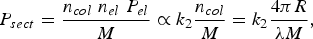(4) $${P_{sect}} = \displaystyle{{{n_{col}}\; {n_{el}}\; {P_{el}}} \over M} \propto {k_2}\displaystyle{{{n_{col}}} \over M} = {k_2}\displaystyle{{4\pi R} \over {\lambda M}}, $$

where n _el is the number of elements per column, P _el is the single Tx element peak power, and k ₂ is the factor that summarizes the other parameters, as above. Increasing M, the beamwidth of each subarray tends to the angular size of the sector obtaining the azimuth coverage of 360° in transmission. The higher M, the higher the signal-to-noise ratio (SNR) single pulse loss due to sector gain and peak power reduction, calling for longer dwell-times compensating for this loss. The SNR loss are computed versus M in dB referred to the “conventionally lossless” case M = 4, (we assume that it is preferable not to use less than four sectors to limit the antenna loss due to the element factor of the elements farther from the central one):

(5) $$\eqalign{SN{R_{loss}} & = 10\; {\rm log}\left( {\displaystyle{{k\; P_{sect}^{(M)} \; G_{sect}^{(M)} } \over {k\; P_{sect}^{(4)} \; G_{sect}^{(4)} }}} \right) \cr & \quad = 10\; {\rm log}\left( {\displaystyle{{4\pi R} \over {\lambda M}}{k_1}\displaystyle{{{n_{col}}\; {\rm sin}(\pi /M)} \over {2\pi }}\; \displaystyle{{\lambda 4} \over {4\pi R}}\displaystyle{{2\pi } \over {\; {n_{col}}\; {\rm sin}(\pi /4)}}} \right) \cr & \quad = 10\; {\rm log}\left( {\displaystyle{8 \over {\sqrt 2 \; M}}{\rm sin}\left( {\displaystyle{\pi \over M}} \right)\; } \right)\; ({\rm dB)},} $$

having assumed k ₁ = 1.

Figure 8 shows the SNR loss with M varying from 4 to 30. On the same plot are shown, versus M, the sector azimuthal size and the related subarray beamwidth. The azimuthal beamwidth depends on the antenna size (R/λ), equation (2), and this particular plot is related to the antenna characteristics of the system [Reference Billetter1] for which R is approximately equal to 25 λ, while the SNR loss is quite general. When M tends to 30 the subarray's beamwidth tends to the sector's azimuthal size realizing an omnidirectional azimuth coverage. Under this condition the loss (17 dB) requires longer integration time to integrate the same energy as with less sectors. However, in some applications the needed integration time may be larger than the transit time of a moving target in a range cell, thus calling for suited processing for the compensation of range-cell migration [Reference Orlando, Ricci and Bar-Shalom24, Reference Li, Yang and Huang25]. The number of samples to be integrated is analyzed in the following.

Fig. 8. Beamwidth, sector angular size, and single-pulse SNR loss versus the number M of sectors.

C) Dwell-time and number of pulses

In this section, applying the search radar equation [Reference Barton26], a lower bound for the maximum time, t _s , for the completion of an activity in a given solid angle, Ω _s , is derived. The case study is related to the d-Radar, for which the transmitting antenna dimension are: R ~ 25 λ, H ~ 6.5 λ, assuming the Tx modules peak power to be equal to 10 W (which is a reasonable value nowadays) and assuming a surveillance solid angle Ω _s of the full 360° in azimuth and 0–70° in elevation. Notice that the d-Radar has a number of operating modes whose description is beyond the aim of this paper, where we limit ourselves to mention the most demanding ones, i.e. the surveillance with track-while-scan of all targets in the coverage area, with a data renewal interval between 1 and 6 s, and the “dedicated tracking” for anti-aircraft artillery, with a data renewal of 100 ms. Each sector has to scan into a Ω _s /M wide solid angle in t _s seconds. Then, the higher M, the higher becomes the dwell-time and the number of pulses. These parameters have been derived for two typical surveillance functions, long range and close range, as defined by the solid angles for medium-range (about 60 km) and short-range (about 25 km) point defense, respectively.

Typical results are shown in Fig. 9 and in Fig. 10, where unambiguous range measurement is assumed.

Fig. 9. Long range and close range search: dwell-time t _d versus sectors number, M.

Fig. 10. Long range and close range search: number of pulses N _dwell versus sectors number, M.

The values in Figs 9 and 10 directly result from the time-power budget as evaluated by the surveillance (and dedicated tracking) radar equation, as an upper bound of the radar performance, and may significantly differ from the real ones. In fact, the real operational values result from a proper waveform design (including the timing, the coverage of blind zones due to eclipsing and many other aspects). In particular, the processing needed for Doppler resolution, clutter mitigation, range adapted waveforms, etc., will cause greater dwell-time's values than the ones in Fig. 9, as well as for the number of pulses in Fig. 10. A detailed design strategy about this trade-off is out of the aim of this paper. Rather, it is interesting to notice that the curves related to the long range/close range functions, with the same behavior, show a quite large difference. Increasing M, a too long integration time may be a limit in some circumstances: a technique for compensating “resolution cell migration” of moving, and maneuvering targets is necessary, with a proper balance between coherent and non-coherent integration. On the other hand with M increasing good low probability of intercept (LPI) property is reached as due to spreading of the energy in time and space. A simple, final consideration results from the examination of Figs 9 and 10: a large number of sectors, i.e. a quasi-ubiquitous radar, is probably the best for close range radar functions, as in a close-in weapons system and with low elevation, pop-up threats [Reference Harman and Hume11–13, Reference Rabideau and Parker21–Reference Qing-long, Yue, Jian and Zeng-ping23](http://www.srcinc.com/what-we-do/radar-and-sensors/lcmr-counterfire-radars.html http://www.srcinc.com/what-we-do/radar-and-sensors/lstar-air-surveillance-radar.html. http://www.srcinc.com/what-we-do/radar-and-sensors/aesa50-multi-mission-radar.html, http://www.srcinc.com/what-we-do/radar-and-sensors/omni-directional-weapon-locating-radar.html).

IV. THE D-RADAR RESOURCES MANAGEMENT

An interesting challenge in the design of a conformal phased array multifunction radar (such as the d-Radar) is the resources management. Figure 11, from [Reference Madia and Maestrini3], shows the general block diagram of the d-Radar.

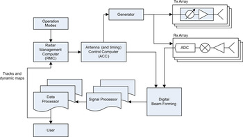
Fig. 11. General block diagram of the d-Radar.

The management of the radar resources is performed by the radar management computer (RMC), which has in its input each operational mode as defined by the operator, and the scenario information (tracks, clutter, and jammer maps) as provided by the data processor. Accordingly, the RMC, first of all, defines a list of activities to be executed, each one with its priority. Priorities are assigned using a multi-criteria procedure: for tracking activities, aimed to fire control or missile control, criteria are based on the threatening of each target, while for surveillance activities, criteria depend on their “relevance” (e.g. the distance from the radar). The ensuing step consists in the definition of the azimuthal sectors in which the beams are aimed by the antenna control computer (depending on the azimuthal distribution of the targets) and in the scheduling of the various radar activities, in order to define the optimal time plan for each activity. The sectors definition and the scheduling are the main differences with respect to a fixed faces radar, in which separate activity scheduling for each face is needed, see Fig. 12.

Fig. 12. Activities management and scheduling; (a) fixed-faces MFAR, (b) conformal MFAR (d-Radar) – The input “op. mode” is the operational mode set by the officer in charge.

It may happen that in a particular scenario (e.g. with many targets under dedicated tracking) the available time is not sufficient to allocate all the activities, and the scheduling algorithm has to perform a forward/backward shift of the activities starting from those with less priority. Scheduling optimization is a well-known field of research, with a wide literature in the multifunction radar context, inter alia: in [Reference Miranda, Baker, Woodbridge and Griffiths27] a comparison between scheduling algorithms is shown, in [Reference Mir and Guitoni28] a scheduling algorithm is proposed with a short description of the state of the art, in [Reference Stromberg and Grahn29–Reference Mir and Abdelaziz34] different scheduling methods are treated. Also in this respect, the d-Radar enables new opportunities with the respect to fixed-faces MFAR: the variable number of simultaneous transmission beams in azimuth (i.e. sectors, between four and ~30), permits to exploit parallel tasks in different sectorsFootnote ² . Moreover, each antenna azimuthal sector can be divided into vertical sections to form many beams at the same azimuth and different elevations. Finally, against pop-up targets, or in general, short range threats, the transmitting array can be moved toward the omnidirectional (staring) mode approaching the ubiquitous radar concept as described previously.

The d-Radar's inherent flexibility, while increasing the operational capacity as compared with more traditional radar architectures, calls for innovative Radar Management algorithms aimed to solve multi-dimensional optimization problems. The scheduling is their core: it has to allocate in a time-frame (e.g. in 6 s) all the radar tasks repeated with their correct update intervals, maximizing the parallel execution of tasks. The number of sectors, M, in which the antenna is divided influences the maximum number of parallel tasks, with some hypothesis and definitions being assumed in the following. We define a task as a basic radar activity composed by the transmission and reception of a waveform in a given direction. Each task belongs to a specific radar function (i.e. close range search, long-range search, detection confirmation, tracking for anti-aircraft artillery or missile guidance etc.) and has its own dwell-time, including the necessary transmission-wait-reception intervals which depend on the distance of the target. In this paper, for the sake of simplicity, a dwell-time is intended to contain all the whole group of n transmitted and received pulses, n being defined according to the processing needs. The update interval equals the repetition time of the task, depending on the requirements of the function to which the task belongs: typically for search purposes the update interval can be of the order of seconds (e.g. 2 s for short range search, 6 s for long-range search) and for dedicated tracking activities it can be of the order of hundreds of milliseconds (e.g. 100 ms for the anti-aircraft artillery function and 1 s for missile guidance).

Tasks belonging to the same radar function have the same update interval. A radar function is composed by several tasks: in surveillance, as many tasks as the number of pointing directions are necessary to cover all the search solid angle; for the tracking functions, the number of tasks is equal to the number of tracked targets; finally, the number of plot confirmation tasks depends on the number of new detections to be confirmed. Each task is defined by its dwell-time, d, its update interval, u, and its pointing direction, θ and ϕ (azimuth and elevation). As described before, an azimuth direction is defined using a particular subset of antenna columns, and the elevation is obtained with the proper phase-shift between the columns elements. So, we denote the pointing direction with an identifier, i.e. an integer number s, which uniquely defines the subarray needed for transmission and reception in the desired θ-direction (no info about elevation is added here since it has no effects on the following). We can assume that, at any time, the radar management computer generates a list of tasks to be executed, and the scheduling method attempts to deliver the optimal timeline solution. If the attempt fails, some tasks must be shifted in time (increasing or decreasing the update interval) or the search tasks dwell-time must be reduced (the obvious consequence being a range reduction). Then, a prioritization ordering is necessary to know the tasks to which the tuning (update interval and dwell-time) can applied first. Moreover, a scenario evaluation is needed to choose the optimal number of antenna sectors (M).

The algorithm method starts after the prioritization and antenna-into-sectors division, so we can assume to have a list of tasks with assigned priorities and all the known parameters (d, u, and s).

An optimization model has been developed [Reference Mir and Wilkinson31], but it falls into the mixed-integer problem category, with a NP-hard solution and a great computational load. In the following, a heuristic solution is proposed in order to obtain a solution to the scheduling problem with the hypothesis that the radar management computer provides a list of tasks each one with its own priority and with the optimal number of antenna sectors M as derived from the evaluation of the scenario. The additional assumption holds of a priori definition about the priority list among the radar functions, for example: if at a given time the active radar functions are long-range search, tracking and plots confirmation, then the inter-functions priority is: (1) tracking, (2) plots confirmation, and (3) long-range search. Therefore, the resulting prioritized queue contains all the tasks. It is necessary to set the time sequence on which the tasks are allocated and to decide to which tasks the update interval and dwell-time adjustments are first applicable. The iterative method starts by allocating the tasks belonging to the function with the highest priority and allocating the repetition of the highest priority task, allowing parallel execution of other suitable tasks, i.e. those with non-overlapping subarrays and equal dwell-time. This operation is iterated with all the lower and lower priority tasks of the first function. Once all the tasks are allocated, the same method is applied to the tasks of the second lower priority function and so on. If at any time one or more repetitions of a task are not allocable due to an overlapping with another task execution, the algorithm attempts to adjust the interval update by shifting forward or backward the starting time. If the task is still not allocable, the algorithm attempts to reduce its dwell-time, otherwise the task is dropped. The update interval and dwell-time adjustments are limited to comply with the pertaining maximum allowed values. By a proper setting of these values one can obtain a feasible time scheduling for a given function. For example, if the dedicated tracking has some hard time constraint, its maximum adjustments values will be set equal to zero, and its function priority level will be the highest, with the consequence that the time resources will be balanced by a range reduction of the surveillance function.

In the following scheme the steps of the method are shown.

In the following section, a typical test of the method with different scenarios is described, varying the number of targets (i.e. the number of dedicated tracking tasks to be scheduled) with a given set of active radar functions and related properties.

A) A study case

The performance of the proposed scheduling method has been evaluated versus the burden posed by a typical operational scenario, determining the maximum number of targets which saturates the radar resources. The simulation trials were carried out considering the following radar functions: long range surveillance up to a range of 70 km (and an elevation up to 25 km, from 0° to 70°), dedicated tracking up to a range of 40 km and, finally, plot confirmation. A function applied to a particular target corresponds to one or more tasks; in turn, each task is made up by a number of looks, each one aimed to a given direction and with a given dwell time. The following hypotheses are assumed for the simulation trials: (i) parallel tasks are permitted only if they belong to the same radar function and have equal dwell-times; (ii) parallel tasks can be exploited using only equal-characteristics and simultaneously non-overlapping subarrays.

Moreover, it is assumed that (i) the Tx antenna is divided into four sectors; (ii) the radar operates without range ambiguities; (iii) the surveillance update time is 6 s with variable dwell-times depending on the elevation direction; and (iv) the dedicated tracking update-time is 100 ms (needed for artillery guidance). The number of “looks” to cover all the search solid angle is equal to 950 (i.e. 780 at low elevation, 0°–20°, and 170 at high elevation, 20°–70°). The time needed to execute the search in the whole solid angle (with dwell-times t _d1 = 20 and t _d2 = 10 ms in low and high elevation, respectively) is:

$${t_s} = \displaystyle{{780} \over 4}{t_{d1}} + \displaystyle{{170} \over 4}{t_{d2}}.$$

The dedicated tracking tasks are scheduled first, having highest priority and a dwell time of 10 ms. After them, with lower priority, are scheduled the plot confirmation tasks. Finally the surveillance tasks are scheduled exploiting the remaining time.

First trials were implemented running the scheduling procedure on the scenario under test and evaluating the number of the dropped tracking tasks. The scenario was modified varying the number of targets to be tracked with dedicated tracking from 10 to 70, assuming a random uniform distribution in azimuth and in range.

Note that every target is managed without any off-boresight beam steering, because the beam is always generated from a sector of the Tx antenna “centerd” on the target direction. Moreover, if the targets in the same beam are more than one, then they are considered all scheduled, thanks to the capability of d-Radar to manage more than one target in the same Tx beam.

One hundred runs of the simulation for each value of the number of targets were done to obtain a reasonable statistical significance of the results. Figure 13 shows some first results concerning the comparison with a classical four-planar-faces phased array radar.

Fig. 13. Percentage of dropped tracking tasks versus the number of targets.

In the case of the four-face phased array the dwell-time changes with the azimuth angle to compensate for the loss in the antenna gain due to the off boresight pointing, starting from the minimum value of 10 ms at the boresight. The corresponding loss explains the distance between both curves in Fig. 13.

V. D-RADAR: CAPABILITIES AND PERSPECTIVES

The d-Radar, based on a bistatic architecture (separated transmitting and receiving conical phased arrays antennas) with and digital beam forming, presents significant advantages with respect to a planar phased array radar when a full 360° coverage is required. This architecture, together with an enhanced usage of the time-energy resources, allows the implementation of simultaneous radar functions, including long-range and close-range surveillance and tracking of multiple targets, and is open to other applications such as air traffic and weather surveillance. The dynamic partitioning of the Tx antenna into subarrays permits the choice of the appropriate number of transmitting beams thus adapting the radar operation to the environment and to the threat. The conical array made up by “columns” symmetrically operating at zero off-boresight angle in azimuth is intrinsically wide-band (measured bandwidths were over 20% and up to 40% of the carrier frequency) permitting frequency agility and diversity with no need to compensate squint errors nor to use true time delay techniques. The absence of any beam revolution during the dwell-time, coupled with the possibility to increase the dwell-time as much as needed, permits a micro-Doppler analysis of targets [35] and, more important in surveillance and defense applications, grants a high correlation of the clutter echoes, especially those from land, with the possibility of a larger improvement factor and a better clutter suppression with respect to scanning radars and to short-dwell time, single beam-per-face phased array radars. This feature is particularly interesting, among others, in (a) air target detection and track-while-scan in the presence of wind farms [Reference Perry and Biss36], and (b) “dry” (i.e. without precipitation) wind shear [Reference Menitt, Klingle-Wilson and Campbell37] monitoring and alerting in airports where the ground clutter is often the limiting factor. In the civil sector, the multifunction capability of the d-Radar architecture potentially satisfies, with a single radar set in X band, the requirements (Damiano Neri (ENAV), Private Communication, Jan. 27th, 2016) of the following applications, today exploited with five different types of radar:

1. (a) Medium range (up to 90 km) and medium elevation (up to 3 km): Air traffic and weather surveillance in the Approach sectors.

2. (b) Short range (up to 9 km) and low elevation (up to circa 150 m): Surveillance of Airport movements (surface movements radar), of wind shear and of bird strike phenomena.

Concerning the d-Radar method of operation, many research and development topics remain to be investigated. To mention a few:

• – Interference between simultaneous beams, and related mitigation means.

• – DBF.

• – Ubiquitous radar mode: practical feasibility with respect to the decorrelation of the target echo during the integration time and the range-cell migration, potential for track-before-detect, advantages in one or more radar activities.

• – Waveform design, including continuous wave, noisy or noise-like waveforms.

• – SIMO and MIMO operations.

• – Low probability of intercept performance.

• – Performance against disturbance due to wind turbines.

• – Wind shear detection and monitoring.

Further possible studies and the feasibility analysis include: (i) defining M simultaneous antenna sectors with different number of columns; (ii) varying M into a single time-frame; (iii) scheduling parallel tasks belonging to different radar functions; (iv) vertical partitioning of the sectors (for dealing with targets at the same azimuth but at different height); (v) operation, in clear and in clutter, with weak and distributed (volumetric) targets such as the tracers (dust, insects [Reference Alistair Drake and Reynolds38], etc.) of the wind shear phenomenon; (vi) wind farms interference suppression. Moreover, future study could consider the d-Radar behavior when a simultaneous azimuthal coverage is achieved by using a high number of antenna sectors (ubiquitous radar), analyzing the benefits and the related optimal resource management and scheduling.