NOMENCLATURE
- a ∞
-
free-stream speed of sound [m/s]
- c
-
blade root chord [m]
-
 $C_p = \frac{p}{\frac{1}{2}\rho _\infty V_\infty ^2}$
-
pressure coefficient [-]
- D
-
propeller diameter [m]
- f
-
frequency [Hz]
- IX, IY
-
TF points indeces [-]
-
$J=\frac{V_\infty }{n \cdot D}$
-
propeller advance ratio [-]
-
$\text{M}_{h,{{\it TIP}}} = \sqrt{\text{M}_{{\it TIP}}^2 + \text{M}_\infty ^2}$
-
tip helical Mach number [-]
-
$\text{M}_{{\it TIP}} = \frac{V_{{\it TIP}}}{a_\infty }$
-
tip Mach number [-]
-
$\text{M}_\infty = \frac{V_\infty }{a_\infty }$
-
free-stream Mach number [-]
-
$n=\frac{{\it RPM}}{60}$
-
propeller angular velocity [rounds/s]
- N
-
propeller geometric periodicity index [-]
- N b
-
propeller number of blades [-]
- p(x)
-
pressure field [Pa]
- p(x, t)
-
pressure time signal [Pa]
- p′(x, t)
-
unsteady pressure time signal [Pa]
- p ref
-
acoustic pressure reference for the SPL [Pa]
- r
-
blade radial coordinate [m]
- R
-
propeller radius [m]
-
$\text{Re}_{{\it TIP}} = \frac{V_{{\it TIP}} \cdot c \cdot \rho _\infty }{\mu }$
-
tip Reynolds number [-]
- V TIP
-
propeller tip speed velocity [m/s]
- V ∞
-
free-stream velocity [m/s]
- x
-
vector position
- x, y, z
-
spacial coordinates [m]
- x w , y w , z w
-
wing spacial coordinates [m]
- z f
-
fuselage longitudinal coordinate [m]
- Δ(·)
-
variation of (·)
- Θ
-
fuselage azimuthal coordinate [deg]
- μ
-
viscosity [Pa·s]
- ρ∞
-
free-stream density [kg/m3]
- ψ b
-
blade azimuthal position [deg]
- ASPL
-
A-weighted SPL
- BPF
-
Blade Passing Frequency
- CFD
-
Computation Fluid Dynamics
- FFT
-
Fast Fourier Transform
- FWH
-
Ffowcs Williams-Hawkings
- OASPL
-
Overall A-weighted SPL
- OSPL
-
Overall SPL
- PSD
-
Power Spectral Density
- RPM
-
Revolutions Per Minute
- SPL
-
Sound Pressure Level
- TF
-
Transfer Function
- TL
-
Transmission Loss
- (·) max
-
Maximum value of (·)
- (·) rms
-
Root Mean Square of (·)
-
$\widehat{(\cdot)}$
-
Fourier transform of (·)
-
$\overline{(\cdot)}$
-
Time average of (·)


Greek Symbol
Acronyms
Subscript and Superscript


1.0 INTRODUCTION
1.1 Motivation and objectives
The aviation industry aims for safer, cleaner and quieter aircraft. For example, the European targets for 2050(Reference Argüelles1-Reference Darecki, Edelstenne, Enders, Fernandez, Hartman, Herteman, Kerkloh, King, Ky, Mathieu, Orsi, Schotman, Smith and Wörner3) are setting reductions in CO 2 and NO x emissions per passenger per kilometre by 75% and 90%, respectively, as well as a cut in the perceived acoustic emissions of flying aircraft by 50% by 2020(Reference Argüelles1), achieving a total noise abatement of 65% by 2050(Reference Darecki, Edelstenne, Enders, Fernandez, Hartman, Herteman, Kerkloh, King, Ky, Mathieu, Orsi, Schotman, Smith and Wörner3). Due to their high propulsive efficiency, propeller-driven aircraft are ideal for economic short and medium range flights, which represent up to 95% of the routes in the European market. Generating thrust from a larger mass flow, propellers allow up to 30% savings in fuel burn with respect to an equivalent turbofan engine, nowadays achieving a similar speed. Moreover, turboprops need shorter take-off/landing lengths and climb time, making them preferable for operations from smaller regional airports and inner city airports with a short runway.
Under the ongoing economic and environmental pressure, the challenge is to find a propeller design that emits lower noise, without a high penalty on performance. For these reasons, Dowty Propellers launched the IMPACTA project(4) (IMproving the Propulsion Aerodynamics and aCoustics of Turboprop Aircraft), in collaboration with the Aircraft Research Association (ARA), the Netherlands Aerospace Centre (NLR), and the University of Glasgow. Innovative blade geometries and hub configurations were studied with the main aim of reducing and/or modifying the acoustic spectra generated by the whole propulsion system. During the project, numerical simulations and scaled wind-tunnel tests were performed to analyse the different propellers in isolation as well as installed by including an engine nacelle and a stub wing.
This paper describes a first part of the work carried out by the CFD Laboratory of the University of Glasgow within the IMPACTA project, focusing on the numerical analysis of the propeller near-field tonal noise in isolated configuration. Reynolds-Averaged Navier-Stokes (RANS) simulations were employed to estimate both the noise incident on the fuselage and the noise perceived inside the cabin, globally evaluating the acoustics of a turboprop aircraft at a low computational cost. Contrary to the Heidmann technique(Reference Heidmann5), which is currently used for aircraft design noise prediction tools (see Ref. 6 for a review of these methods), RANS allow to capture the characteristic acoustic features of different propeller geometries, thus enabling their assessment on the emitted sound spectra and the overall noise level radiated, early in the design stage.
1.2 Propeller noise: Physics and methods
Propeller noise is composed of several tones and a broadband part. The tonal components are related to the Blade Passing Frequency (BPF), at which the highest noise level occurs, and its harmonics. An almost linear decreasing trend is observed in the sound pressure level, with increasing harmonic order(Reference Müller and Möser7). Additional sub-harmonics arise in the noise spectra if there are asymmetries in the blade geometry and/or in the azimuthal blade spacing, thus making the spectra more continuous. At subsonic tip speeds, tonal noise is generated by (i) the periodic flow displacement caused by the finite thickness of the blades and (ii) the periodic variation of blade aerodynamic forces with respect to a fixed observer position. The helical blade-tip Mach number (M h, TIP ) is the main propeller operating parameter for tonal noise. Increasing M h, TIP results in a rapid increase of higher harmonic noise levels. Up to around 0.6–0.7 M h, TIP , for a typical general aviation propeller, the loading noise is the dominant noise generation mechanism, while at higher M h, TIP the thickness noise usually prevails(Reference Müller and Möser7). Loading noise can be described by an acoustic dipole, with its radiation lobes directed forward and backward of the blade disk plane. Directivity peaks of thickness noise, represented by a monopole source, are instead in proximity of the rotational axis, along which no rotational noise is radiated assuming perfectly uniform axial inflow conditions. Broadband noise results from the interaction between the propeller blades and turbulent flow, as well as from blade trailing-edge noise. It can be modelled as an acoustic dipole whose axis is perpendicular to the blade chord, thus its contribution in the total aircraft noise signature is not significant for a horizontal flyover(Reference Müller and Möser7), at least in the near field. Under non-uniform and/or unsteady inflow conditions (e.g. climb or disturbed flow due to installation effects), the noise increases and its directivity pattern and dependence on the tip Mach number differ from the ideal inflow case. By means of a spectral conditioning technique, it was recently shown that the tonal noise can vary by up to 8 dB as a consequence of unsteady loading and that this effect is stronger in the upstream than in the downstream direction(Reference Carley and Fitzpatrick8). The periodic non-uniform rotational motion of piston engines also causes unsteady flow conditions over the propeller blades. This results in a modulation of the noise spectra if there is coincidence between BPF tones and the engine crank frequency, or in additional harmonics in the case of no interference between the two frequencies(Reference Yin, Ahmed and Dobrzynski9).
Most of the currently used propeller acoustic prediction techniques deal only with the tonal component of the noise. A first analytical expression of radiated sound energy and directional properties for the lower propeller harmonics, under static conditions, was derived by Gutin(Reference Gutin10) in 1936. In the following years, extensions of Gutin’s work were made to include higher harmonic noise(Reference Deming11), blade thickness, thrust and torque contributions(Reference Deming12) and forward flight conditions(Reference Garrick and Watkins13). In the early 1950s, Lighthill published the ‘Acoustic Analogy’(Reference Lighthill14,Reference Lighthill15) , base of most modern aeroacoustic theories, including the Ffowcs Williams-Hawkings (FWH) equation(Reference Williams and Hawkings16) presented in 1969 and nowadays still employed for rotor and propeller farfield noise predictions, in the time domain following Farassat’s formulations(Reference Farassat17) or in the frequency domain(Reference Hanson18,Reference Hanson and Parzych19) . Because of the computational requirements and the related issues of computational aeroacoustics (see Refs 20–22 for a detailed description), the direct noise computation for propellers is still excessively expensive and time-consuming; thus, the current approach is to couple a CFD method in the nearfield with an acoustic solver to propagate the noise in the domain far-field. Single-blade RANS and DES computations were used by De Gennaro et al(Reference De Gennaro, Caridi and Pourkashanian23,Reference De Gennaro, Caridi and De Nicola24) and Tan and Alderton(Reference Tan, Voo, Siauw, Alderton, Boudjir and Mendonça25), respectively, coupled with Brentner and Farassat’s formulation of the FWH equation(Reference Williams and Hawkings16,Reference Brentner and Farassat26) , to predict tonal noise of the NASA SR2 blade(Reference Dittmar and Lasagna27,Reference Whitfield, Gliebe, Mani and Mungur28) . Good agreement with experimental data was found with both methods, the second improving the accuracy at rear locations. RANS were also proved a succesful tool in optimising the propeller blade shape as shown in the research of Marinus et al(Reference Marinus, Roger and Van de Braembussche29,Reference Marinus30) . Finally, RANS simulations are also employed to compute contra-rotating open rotors (e.g. Refs 31–33) and marine propellers (e.g. Ref. 34).
Regarding the broadband noise, a general and global model is not yet reported and thus scaling noise laws(Reference Skvortsov, Gaylor, Norwood, Anderson and Chen35) and semiempirical approaches based on specific source mechanisms (e.g. Proudman’s method(Reference Proudman36,Reference Lilley37) or models derived from exact solutions of flat-plate acoustic scattering problems(Reference Amiet38-Reference Rozenberg42)) are usually adopted (see, e.g. the approaches used in Refs 43 or 44). In this work, the broadband noise contribution is not modelled.
1.3 Paper outline
In the following, first the CFD solver, used in this work, is described and validated for flow around propellers (Section 2). The IMPACTA propeller geometries are then presented in Section 3, together with a description of the computational grids and of the test cases. In Section 4, the acoustic analysis of the different designs is carried out. Overall Sound Pressure Level (OSPL) and Sound Pressure Level (SPL) spectra in the frequency domain are first compared. After that, an evaluation of the noise inside the cabin is performed through the application of transfer functions. Finally, Section 5 provides some conclusions of this work and presents future developments of the research.
2.0 CFD FLOW SOLVER HMB3
Numerical simulations were performed using the in-house parallel CFD solver Helicopter Multi Block (HMB3)(Reference Barakos, Steijl, Badcock and Brocklehurst45,Reference Steijl, Barakos and Badcock46) . HMB solves the 3D Navier-Stokes equations in dimensionless integral form using the Arbitrary Lagrangian Eulerian (ALE) formulation for time-dependent domains with moving boundaries:
 $$\begin{equation}
\frac{d}{dt}\int _{V(t)}\mathbf {w} dV + \int _{\partial V(t)}(\mathbf {F}_i (\mathbf {w}) - \mathbf {F}_v (\mathbf {w})) \cdot \mathbf {n} dS = \mathbf {S},
\end{equation}$$
$$\begin{equation}
\frac{d}{dt}\int _{V(t)}\mathbf {w} dV + \int _{\partial V(t)}(\mathbf {F}_i (\mathbf {w}) - \mathbf {F}_v (\mathbf {w})) \cdot \mathbf {n} dS = \mathbf {S},
\end{equation}$$
where V(t) is the time dependent control volume, ∂V(t) its boundary, w is the vector of the conservative variables (ρ, ρu, ρv, ρw, ρE) T , F i and F v are the inviscid and viscous fluxes, respectively, and S is the source term.
The viscous stress tensor is approximated using the Boussinesq hypothesis(Reference Boussinesq47,Reference Pope48) and several turbulence closure models are implemented, among which the k − ω(Reference Wilcox49) and the k − ω SST(Reference Menter50) that are used in this work. The Navier-Stokes equations are discretised using a cell-centered finite-volume approach. A curvilinear co-ordinate system is adopted to simplify the formulation of the discretised terms, since body-conforming grids are adopted. The system of equations that has to be solved is then:
 $$\begin{equation}
\frac{d}{dt}\left(\mathbf {w}_{i,j,k} {\cal {V}}_{i,j,k}\right)+\mathbf {R}_{i,j,k} = 0,
\end{equation}$$
$$\begin{equation}
\frac{d}{dt}\left(\mathbf {w}_{i,j,k} {\cal {V}}_{i,j,k}\right)+\mathbf {R}_{i,j,k} = 0,
\end{equation}$$
where w
i, j, k
is the vector of conserved variables in each cell,
 ${\cal {V}}_{i,j,k}$
denotes the cell volume and R
i, j, k
represents the flux residual. Osher’s upwind scheme(Reference Osher and Chakravarthy51) is used for the convective fluxes because of its robustness, accuracy and stability properties. The Monotone Upstream-centered Schemes for Conservation Laws (MUSCL) variable extrapolation method(Reference van Leer52) is employed to provide second-order accuracy. Spurious oscillations across shock waves are removed with the use of the van Albada limiter(Reference van Albada, van Leer and Roberts53). The integration in time is performed with an implicit dual-time method to achieve fast convergence. The linear system is solved using a Krylov subspace algorithm, the generalised conjugate gradient method, with a block incomplete lower-upper (BILU)(Reference Axelsson54) factorisation as a pre-conditioner. Boundary conditions are set by using ghost cells on the exterior of the computational domain. To obtain an efficient parallel method based on domain decomposition, different methods are applied to the flow solver(Reference Lawson, Woodgate, Steijl and Barakos55) and the Message Passing Interface (MPI) tool is used for the communication between the processors.
${\cal {V}}_{i,j,k}$
denotes the cell volume and R
i, j, k
represents the flux residual. Osher’s upwind scheme(Reference Osher and Chakravarthy51) is used for the convective fluxes because of its robustness, accuracy and stability properties. The Monotone Upstream-centered Schemes for Conservation Laws (MUSCL) variable extrapolation method(Reference van Leer52) is employed to provide second-order accuracy. Spurious oscillations across shock waves are removed with the use of the van Albada limiter(Reference van Albada, van Leer and Roberts53). The integration in time is performed with an implicit dual-time method to achieve fast convergence. The linear system is solved using a Krylov subspace algorithm, the generalised conjugate gradient method, with a block incomplete lower-upper (BILU)(Reference Axelsson54) factorisation as a pre-conditioner. Boundary conditions are set by using ghost cells on the exterior of the computational domain. To obtain an efficient parallel method based on domain decomposition, different methods are applied to the flow solver(Reference Lawson, Woodgate, Steijl and Barakos55) and the Message Passing Interface (MPI) tool is used for the communication between the processors.
An isolated rotor in axial flight conditions is simulated as a steady flow problem, assuming the shed wake steady, and the flow periodic in space and time. Besides, the azimuthal periodicity of the flow is used to resolve only one segment of the computational domain, applying periodic boundary conditions, thus further reducing the computational effort. The problem is formulated in a non-inertial frame of reference, modifying the ALE formulation (1) to account for the centripetal and Coriolis acceleration terms appearing via a mesh velocity, which corresponds to a solid-body rotation of the grid in the direction of the rotor rotation ω, and a momentum source term(Reference Steijl, Barakos and Badcock46). Two different approaches are used in HMB to apply the far-field boundary conditions. A linear extrapolation in the normal direction on the inflow and outflow boundaries is adopted where the computational domain is extended sufficiently far away from the propeller to avoid the presence of numerical flow re-circulation if free-stream boundary conditions are imposed. Froude’s ‘potential sink/source’ approach is employed elsewhere(Reference Biava and Vigevano56).
2.1 HMB3 validation for propellers
HMB3 has been validated for propeller flows, using the Joint Open Rotor Program (JORP)(Reference Scrase and Maina57) and the IMPACTA(4,Reference Gomariz-Sancha, Maina and Peace58) wind-tunnel data. The JORP database allows a comparison of blade pressure distribution in a propeller isolated configuration. The IMPACTA measurements instead, enable an aerodynamic and acoustic validation for an installed case with a wing behind the propeller.
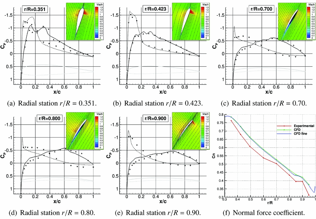
The JORP model was a single row, six-bladed propeller, mounted on a minimum interference spinner, representative of a high-speed design of the late 1980s. Simple unswept and moderately swept blade planforms were tested, with a relatively large tip chord. Using the axial flight formulation, RANS simulations of the unswept JORP at fixed pitch were performed, with the k-ω turbulence model(Reference Wilcox49). The single-blade computational domain was extended up to the far-field and the hub was modelled as a cylinder to have a faster convergence of the steady-state simulation. Blade parameters and test conditions are reported in Table 1. Figure 1 shows the pressure coefficient distribution at different radial positions along the blade. A visualisation of the flowfield around the different profiles, with streamlines and Mach colour iso-levels, is also reported in the same figure. Some small discrepancies are visible in Fig. 1, specially regarding the suction peak. This is believed to be due on one hand to the uncertainty in the experimental pitch angle and on the other hand to the fully turbulent CFD model adopted, whereas small laminar regions were observed on the blades during the tests. Nevertheless, the trend of the normal force coefficient along the blade is well-captured. Validation results for this case are more extensively reported in Ref. Reference Barakos and Johnson59.

Figure 1. Pressure coefficient distribution along different stations of the unswept version of the JORP propeller: comparison between numerical results of HMB3 and experimental data(Reference Scrase and Maina57) (triangular points).
Table 1 HMB3 validation: Propeller parameters and test conditions

The IMPACTA wind-tunnel model is a 1 to 4.83 scale model of an installed turboprop power-plant and comprises propeller, nacelle, intake, and part of the wing. The model was tested in the Transonic Wind Tunnel of ARA. The model was mounted upside down in the tunnel section as shown in Fig. 2(a). Figure 2(a) shows the geometry and dimensions of the model (the propeller radius was 0.4572 m). The propeller angular rotation was clockwise, as viewed from the rear, and the axis of rotation, coincident with the grid x axis, which is inclined by −2° with respect to the fuselage axis. The wing pitch angle was 5.3° with respect to the propeller thrust axis. The propeller parameters and test conditions are summarised in Table 1. The structured multi-block CFD grid was built by assembling five separate components (see Fig. 2(b)): the propeller drum, the inflow, the front part of the model, the back part of the model, and the outflow. The sliding plane technique(Reference Steijl and Barakos60) was employed to exchange flow information between the different grids. This allowed (i) the relative motion between the propeller and the rest of the model, (ii) the possibility to change the propeller design without modifying the rest of the grid, and (iii) grid topology simplifications and/or the reduction of the number of cells in different parts of the computational domain. To have a perfectly symmetric computational domain, the propeller drum was generated by copying and rotating a single-blade mesh and all other grid components were mirrored about the y = 0 plane. An ‘O’ grid topology surrounds the whole model and a computational mesh spacing that ensures y + ⩽ 1 was adopted, by using a hyperbolic mesh point distribution and a wall grid stretching ratio ranging from 1.1 to 1.15. All geometric details of the wind-tunnel model were represented in the mesh. The wind-tunnel walls were not modelled in the CFD simulations and the far-field boundaries have been extended with respect to the wind-tunnel test thus to apply far-field boundary conditions. This was the case since the experimental data was corrected to take into account the effect of the acoustic liner employed during the tests (refer to Ref. 58 for a short description of the adopted correction procedure).
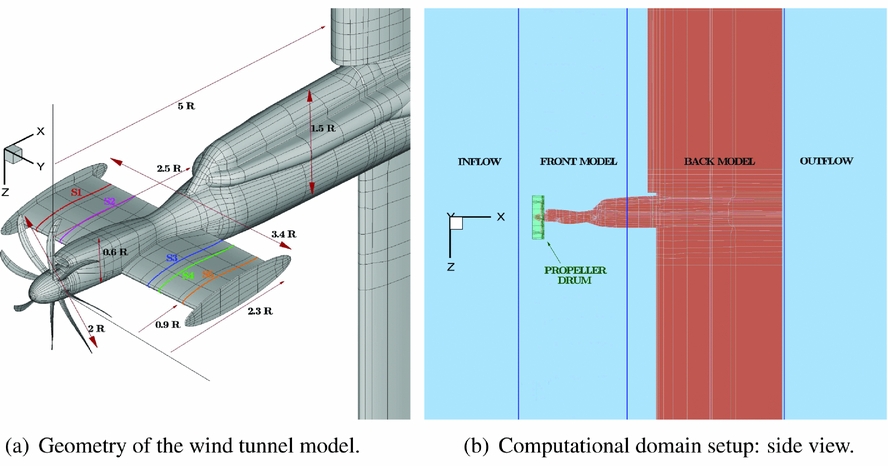
Figure 2. IMPACTA wind-tunnel scaled model with the Baseline propeller design.
k − ω SST(Reference Menter50) unsteady RANS (URANS) computations were performed with a temporal resolution of 360 steps per propeller revolution, i.e. one unsteady step corresponded to 1° of propeller azimuth. The simulations started from undisturbed free-stream flow conditions and four propeller revolutions were needed to obtain statistically time-invariant flow predictions. A coarse grid of 20.1 million cells and a finer grid, with a spatial resolution doubled in all directions, giving a total of about 161.3 million cells, were used. Numerical probes were introduced in the simulations at the cell centres nearest to the position of the unsteady pressure sensors to record the pressure evolution in time and to allow a comparison of the noise spectra.
Average pressure coefficient distributions on the IMPACTA model and a comparison against experimental data provided by ARA for some sections on the wing are shown in Fig. 3. Measurements of the steady pressure sensors were taken on runs of 15 seconds, i.e. ~1,000 propeller revolutions; numerical data were averaged over one revolution. Good agreement between the HMB3 URANS averaged solutions and experimental measurements can be observed, at all stations, and the effect of the propeller slipstream on the wing loading is captured by CFD (see differences in the chord-wise C p distribution between correspondent wing sections on the port and starboard sides). No significant difference is observed between the coarse and the fine grid predictions; thus, it is concluded that, regarding the wing loads, the resolution of the coarse grid is adequate. Figure 4 shows the propeller wake, visualised using the Q-criterion, and the unsteady pressure field, comparing results from coarse and fine grids. Unlike loading predictions, differences in the propeller wake and unsteady pressure field resolution between coarse and fine grids are significant. The coarse grid is still able to preserve the propeller wake at least until it encounters the wing (Fig. 4(a)). However, the fine mesh, as shown in Fig. 4(b), resolves smaller vortical structures and preserves them longer; it also results in tighter vortex cores. The same is noted for the unsteady pressure field: although the coarse mesh (see Figs 4(c) and (e)) shows the differences between the starboard and port sides of the model, dissipation is seen in the propagation of the acoustic waves, which is considerably reduced in the fine mesh (Figs 4(d) and (f)). Finally, a comparison of the SPL spectra against the ARA experimental data for four locations on the wing is reported in Fig. 5. Since the signal length significantly influences the frequency study, only one revolution was considered in the analysis of the signal from the Kulites as the stored numerical signal spans one propeller revolution only. Moreover, the experimental signal was filtered at the CFD Nyquist frequency using a 4th order Butterworth filter(Reference Butterworth61). Some differences between the coarse and the fine grid results are evident. The coarse grid captures up to the second harmonic, while the fine mesh up to the third, with averaged discrepancies of up to 3 dB. However, sensible discrepancies of CFD results are noted for some Kulite, in particular, on the starboard upper wing side. Globally, it is concluded that HMB3 results capture the dominant tones of the near-field acoustics.

Figure 3. Pressure coefficient distribution along different stations of the wing of the IMPACTA Baseline scaled model: comparison between numerical results of HMB3 and experimental data(Reference Gomariz-Sancha, Maina and Peace58) (rectangular points). Please refer to Fig. 2 for the exact location of the different sections.

Figure 4. Flow-field instantaneous visualisation of the IMPACTA wind-tunnel scaled model. Comparison between numerical results of the coarse grid (on the left) and of the fine grid (on the right).

Figure 5. SPL spectra on the IMPACTA wind-tunnel model: comparison between HMB3 numerical results and Kulite measurements(Reference Gomariz-Sancha, Maina and Peace58). In the measurements, broadband as well as tonal sources of pressure fluctuation are included.
3.0 COMPUTATIONAL SETUP
3.1 IMPACTA propellers design
The IMPACTA propeller is a new-generation design, aiming for high efficiency at high speeds. It has eight blades with a radius r of 2.209 m and a chord c of 0.213 m. The sections of the blades are thin, highly twisted and swept back (~50° at 0.7r), and are designed to operate at high loading.
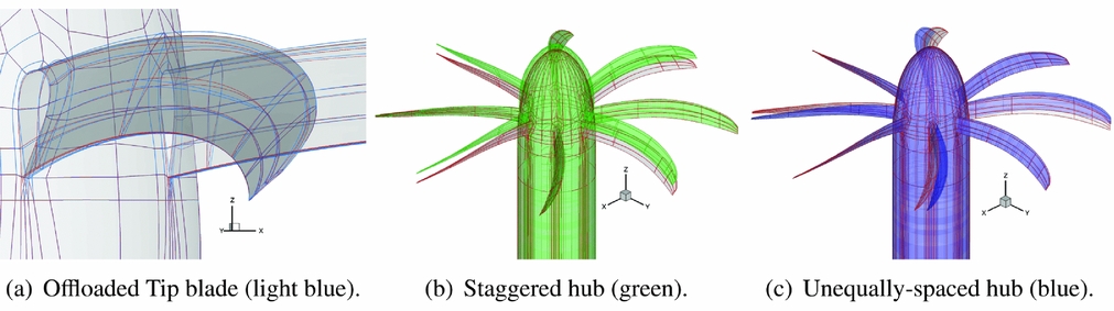
Besides the Baseline propeller, three different propeller designs were considered: an Offloaded-Tip blade, a Staggered hub and an Unequally Spaced hub. The modified geometries, against the Baseline design, are shown in Fig. 6. The three propellers are designed to deliver the same thrust. The Offloaded-Tip blade is characterised by less tip twist and runs at a slightly higher pitch angle than the Baseline design, thus to move the peak of the blade loading inboards. As can be predicted from a simple semi-empirical analysis(Reference Müller and Möser7), this should yield a noise reduction. Moreover, to achieve the same thrust, the Offloaded Tip blade operates at a lower RPM, i.e. at a higher advance ratio, further increasing the blade pitch. Therefore, this design will also benefit from the decrease in the tip Mach number, which results in a significant propeller noise reduction (refer to Refs 62 and 63 that report wind-tunnel or in-flight experimental data showing a decrease in the noise levels of the first tones with decreasing tip speed). The main idea behind the different hub designs is instead a modulation of the noise spectra by changing the geometric periodicity of the propeller to redistribute the acoustic energy on more frequencies. This should result in a more pleasant sound to the human ear. In particular, the Staggered hub has four blades offset towards the spinner tip by 2/3 of the root chord, while the Unequally Spaced hub has the space between the blades modified by ±4°. The Staggered hub is expected to be more efficient and noisier than the Baseline due to the different inflow conditions seen from the second row of propeller blades. The higher efficiency provides also an opportunity to reduce the propeller hub and the spinner diameters for a lower drag installation. Asymmetric blade-spacing was instead shown to yield to noise reduction in some radiation direction(Reference Dobrzynski64) because of interference among the sound emitted from the individual blades.

Figure 6. IMPACTA modified propeller geometries vs Baseline design (grey and red).
The operating cruise conditions for the IMPACTA propellers are reported in Table 2. Note that the Offloaded Tip design will exhibit a lower fundamental frequency because of the lower operating RPM.
Table 2 Cruise operating conditions for the IMPACTA blades
3.2 Test cases
All IMPACTA designs were numerically studied in isolated configuration. Steady RANS simulations were therefore performed, employing the axial flight formulation described earlier. The k − ω SST turbulence model(Reference Menter50) was used to close the RANS equations. From a steady computation, it is not possible to directly capture the broadband noise content, therefore the acoustic analysis will be focused only on the tonal noise. The test cases are summarised in Table 3.
Table 3 Computational test cases
3.3 Computational grids
Multi-block structured grids were generated using the ANSYS-Hexa™ meshing software(65) and a classic ‘C−H’ block topology was employed around the blades. Using the axial flight formulation, only 1/N of the domain was represented, where N is the geometric periodicity index of the propeller. Therefore, N = 8 for the baseline hub configuration (Baseline and Offloaded Tip blades - grids G1 and G2, respectively) and N = 4 for the modified hub configurations (Unequally Spaced and Staggered designs - grids G3 and G4, respectively). The computational domain and the spinner were extended downstream to apply free-stream boundary conditions on the far-field boundaries, accommodating two propeller revolutions with the wake resolved over more that 180°. Figure 7 shows the computational domain, the grid topology, and the surface mesh details of the IMPACTA Baseline design. The different grids were built as similar as possible for all propeller designs, thus to limit the influence of the computational grid on the numerical predictions. Details of the grid dimensions and properties are reported in Table 4. The spacial resolution of the computational grids was chosen on the base of the results of the grid convergence study of the JORP case(Reference Scrase and Maina57,Reference Barakos and Johnson59) . The wall spacing was chosen to ensure a y + ~ 0.5 on average along the blade and values slightly higher than one towards the spinner junction. The grids are quite regular in the area of interest, with stretched cells only in the boundary layer, to perform wall-resolved Navier-Stokes computations, and in the far-field, where a fine spatial resolution is not needed. Mesh quality indices reported in Table 4 are related to the whole grid, including boundary layer and far-field cells.
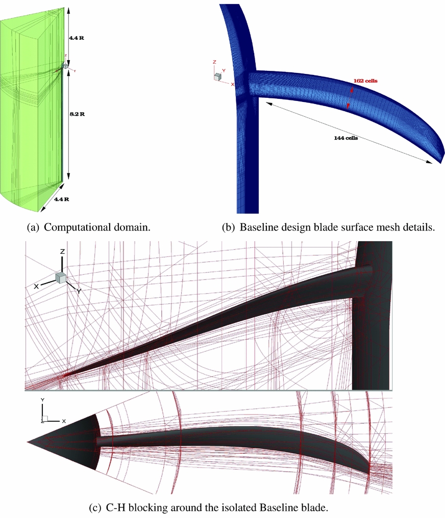
Figure 7. Computational grids for the isolated propeller computations.
Table 4 Dimensions and properties(66) of the IMPACTA isolated blade(s) computational grids.
a Worst values over the whole grid
4.0 DISCUSSION OF THE RESULTS
4.1 Aerodynamic and performance results
Since the aerodynamic characteristics of the different propellers are not the prime focus of this work, it is only noted here that the flow is mostly attached on the whole blade for all the designs. As it can be seen in Fig. 8 for the Baseline blade, the flow separates only in a very small area (Zone A) on the blade root suction side. Because of the propeller noise generation mechanism, it is important to look at the span-wise load distribution. Figure 9 shows the pressure coefficient distribution at three different blade stations for the modified propeller designs with respect to the Baseline. It can be seen that significant differences are predicted only for the Offloaded Tip blade. As expected from the geometric characteristics of this design, the peak loading is moved inboards (see Figs 9(a)–(c)). The modifications of the hub configuration did not lead to any notable effects on the span-wise load distribution. Small differences are seen only towards the blade root.
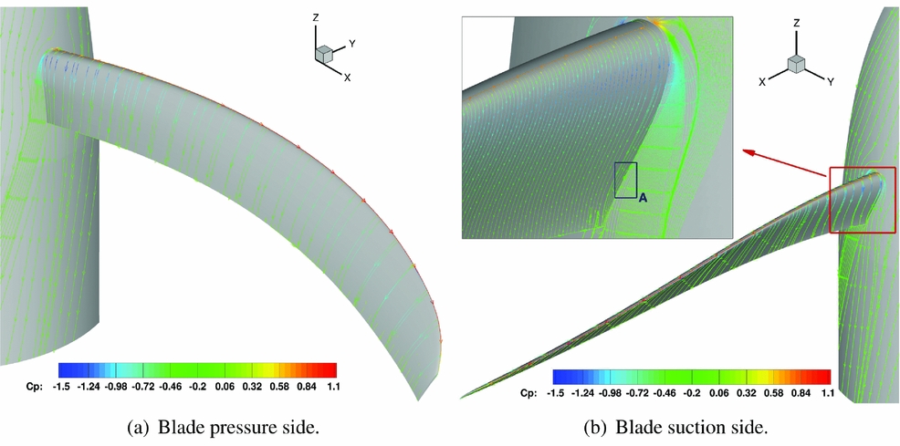
Figure 8. Baseline IMPACTA propeller at cruise conditions: flow visualisation of the propeller through friction, coloured by pressure coefficient.

Figure 9. Chord-wise pressure coefficient distribution at different blade radial stations for the modified IMPACTA designs compared to the Baseline.
It is observed that, at the simulated conditions with fixed pitch, the modified designs provide a different thrust with respect to the Baseline design (see Table 5). Therefore, the noise levels of the different propellers were corrected via semi-empirical approaches to account for the different blade loadings and compare the acoustics at the same thrust. In particular, the procedure described in Ref. 7 based on Ref. 67 was used for the overall A-weighted noise level, while the ESDU method derived from Gutin’s theory(Reference Gutin10,68) was applied to correct the SPL of the various harmonics. Table 5 reports the magnitude of the corrections adopted.
Table 5 IMPACTA propellers thrust with respect to the Baseline design and correspondent noise levels corrections
4.2 Acoustic analysis
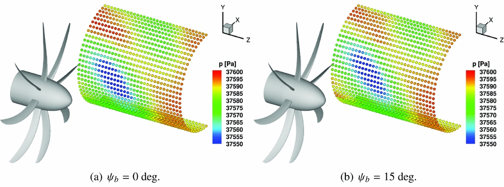
An idealised fuselage representative of a high-wing aircraft was modelled to investigate the noise characteristics of the different designs. An array of virtual microphones, or monitoring points, were arranged in a 32 × 33 matrix of a half cylinder, located approximately 5 chord lengths away from the blade tip and extended 11.5 chord lengths in front and 4 chords behind the propeller rotational plane (see Fig. 10). Figure 11 shows as an example the incident pressure field p(x) on the idealised fuselage for the Baseline design. Two azimuthal blade positions relative to the fuselage were considered, i.e. at two different instances of the equivalent unsteady simulation. To estimate the noise at each selected point, an equivalent one revolution long unsteady pressure signal p(x, t) was reconstructed from the steady CFD solution using a time sampling corresponding to 0.25° of propeller rotation, i.e. according to Nyquist’s theorem(Reference Jerri69), the maximum captured frequency will be about 10 kHz. Overall Sound Pressure and Sound Pressure Levels as functions of the frequency are then computed as follows:
 $$\begin{equation}
OSPL &=& 10 \log _{10}\left(\frac{{p^ \prime _{{\it rms}}}^2}{{p_{{\it ref}}}^2}\right) \text{ dB,}
\end{equation}$$\\
$$\begin{equation}
OSPL &=& 10 \log _{10}\left(\frac{{p^ \prime _{{\it rms}}}^2}{{p_{{\it ref}}}^2}\right) \text{ dB,}
\end{equation}$$\\
 $$\begin{equation}
SPL(f) &=& 10 \log _{10}\left(\frac{PSD(p^ \prime)}{{p_{ref}}^2}\right) \text{ dB,}
\end{equation}$$
$$\begin{equation}
SPL(f) &=& 10 \log _{10}\left(\frac{PSD(p^ \prime)}{{p_{ref}}^2}\right) \text{ dB,}
\end{equation}$$
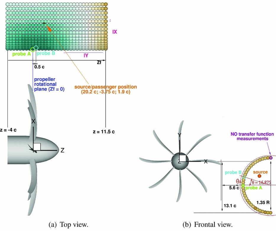
Figure 10. Acoustic analysis setup: idealised fuselage representative of a high-wing narrow-body commercial aircraft.

Figure 11. Baseline IMPACTA propeller: instantaneous incident pressure distribution on the idealised fuselage.
To take into account the hearing sensitivity of the human ear, the A-weighting filter was also applied to the sound pressure estimates. According to standards from Refs 70 and 71, the A-weighted SPL (ASPL) was determined as
 $$\begin{equation}
ASPL(f) = SPL(f) + 20 \log _{10}\left(G_A(f)\right) + 2 \text{ dB}_A\text{,}
\end{equation}$$
$$\begin{equation}
ASPL(f) = SPL(f) + 20 \log _{10}\left(G_A(f)\right) + 2 \text{ dB}_A\text{,}
\end{equation}$$
where G A (f) is the frequency-dependent filter gain
 $$\begin{equation}
G_A(f) = \frac{12200^2 \cdot f^4}{(f^2 + 20.6^2)(f^2 + 12200^2)\sqrt{f^2 + 107.7^2}\sqrt{f^2 + 737.9^2}}\text{ dB.}
\end{equation}$$
$$\begin{equation}
G_A(f) = \frac{12200^2 \cdot f^4}{(f^2 + 20.6^2)(f^2 + 12200^2)\sqrt{f^2 + 107.7^2}\sqrt{f^2 + 737.9^2}}\text{ dB.}
\end{equation}$$
Finally, the Overall A-weighted SPL (OASPL) was computed, considering the contribution of the first five harmonics.
The overall sound pressure levels on the idealised fuselage at cruise operating conditions, and the corresponding OASPL value, are presented in Fig. 12 for all the designs. No substantial differences are seen regarding the trend in the OSPL distribution. The higher noise levels on the idealised fuselage are observed in the proximity of the propeller rotational plane, at about 17° of azimuthal position. There, as it can also be partly seen in Fig. 11, the largest fluctuations of pressure occur. Moving away from this region, in the longitudinal and in the azimuthal directions, the distance from the noise sources increases and the OSPL decreases. In particular, the OSPL peak for the Baseline design is predicted 0.5 chords in front of the propeller rotational plane (probe B in Fig. 10). The Offloaded-Tip blade and the Unequally Spaced hub also show the OSPL maximum at the same position. The Staggered hub design instead exhibits the maximum noise level 0.5c further ahead because of the translation of the first blade-row. The A-weighting filter yields lower noise levels. This is because the filter gains are negative for frequencies below 1 kHz, thus for all the first eight harmonics of the IMPACTA propellers. Moreover, the noise reduction due to the A-weight filter for the Offloaded Tip blade is higher in magnitude than for the other designs because its harmonics are at lower frequencies. With the exception of the Offload Tip design, it is observed that the point of maximum OASPL is found at a fuselage station behind the one where the peak of OSPL is predicted. Regarding the noise levels, the Offloaded Tip blade shows an acoustic footprint significantly quieter than the Baseline design with OASPL max, Offload 6.2 dB A less than OASPL max, Baseline. Both Staggered and Unequally Spaced designs, instead, yield slightly higher noise levels with respect to the Baseline IMPACTA propeller (OASPL max, Staggered = +1.98 dBA, OASPL max, Unequal = +2.31 dBA). It can be noticed that, unlike the OSPL, the OASPL of the Staggered hub is lower than the Unequally Spaced for a big part of the fuselage because of the different distribution of the acoustic energy over the frequencies. This can be better understood looking at the noise spectra.

Figure 12. OSPL and OASPL value up to the fifth harmonic on the idealised fuselage for the different IMPACTA propeller designs. The colour scale range is equal to 30 dB.
Figure 13 shows, as an example, the constant bandwidth SPL spectrum of the Baseline propeller at the nearest point of the idealised fuselage to the blade tip. Tones at the blade passing frequency (BPF = 114.152 Hz) and its multiples are clearly visible, up to the eighth harmonic. The expected linear decay typical of ideal inflow conditions is also observed. The predicted SPL values are in good agreement with estimates provided by the designer(72), with a maximum discrepancy of less then 1.5 dB for the first few tones.
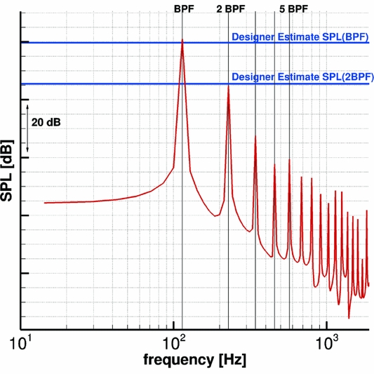
Figure 13. Baseline design at cruise conditions: SPL spectrum at the closest point of the idealised fuselage to the blade tip (z f = 0c, Θ = 16.875).
A comparison between the spectra of the different designs at probe B (see Fig. 10) is reported in Fig. 14. Table 6 reports the sound pressure levels of the first three BPF harmonics of the modified designs scaled by the Baseline propeller at the same location, together with the OASPL level considering up to the fifth harmonic. The Offloaded Tip blade, which, as already explained, shows tones at lower frequencies, is significantly quieter than the Baseline design, with an appreciable noise level reduction up to at least the fourth tone. Both Staggered and Unequally Spaced designs show tones also at multiples of BPFs/2 due to the different geometric periodicity. Their acoustic energy is thus spread over more frequencies, and, in total, they are slightly louder than the Baseline design. Differences in the frequency distribution of the acoustic energy between the Staggered and the Unequally Spaced hubs can be noted: the first has an SPL slightly higher than the second at BPFs tones but significantly lower at BPFs/2 tones, thus resulting in almost the same values of OASPL.

Figure 14. SPL at the point B of the idealised fuselage (z f = 0.5c, Θ = 16.875) for the different IMPACTA propeller designs.
Table 6 Differences in noise levels comparison between the modified designs and Baseline propeller at point B (z f = 0.5c, Θ = 16.875°)
Looking at the noise spectra at different locations on the fictitious fuselage, a sound directivity analysis was carried out. In particular, Figs 15 and 16 show the behaviour of the first three BPF tones along the fuselage axis z f and along the fuselage circumference (i.e. varying the fuselage azimuth Θ). Please refer to Fig. 10 for the locations considered. In general, it is shown that, moving longitudinally, the BPF tone has an almost symmetric behaviour with respect to the fuselage station where the maximum OSPL is registered. Therefore, at the same distance from the propeller plane, the SPL of the BPF is slightly noisier ahead of the propeller than aft. Regarding the second tone, a symmetric behaviour with respect to the propeller rotational plane is noted until about seven chord lengths away. The third tone shows a less clear trend, with a relative peak around the propeller rotational plane. Finally, it can be observed in Fig. 15 that the trends of the various tones are similar at different azimuthal positions. Moving along the fuselage azimuth, Fig. 16 shows that the maximum noise level at BPF and at 2 BPF is around 16–17°, which is the point of minimum distance from the propeller tip; while at 3 BPF, the maximum is at higher Θ values. It has to be noticed that, due to the hypothesis of steady and periodic flow, and the absence of the airframe in the simulation, points at the same radial distance from the propeller tip will show the same SPL. This is expected not to be the case in an installed configuration. Regarding the modified propeller designs, it is observed from Figs 15 and 16 that: (i) the Offloaded Tip blade shows lower noise levels at all positions on the fuselage. This blade produces the same trend as the Baseline design, moving along the fuselage axis, at BPF and a flatter trend at 2 BPF; (ii) with respect to the Baseline propeller, the BPF of the Staggered hub design has a slightly higher SPL in front of the propeller plane and lower SPL behind it, while the 2 BPF tone is quieter in the vicinity of the propeller plane and louder after three chord lengths; (iii) the Unequally Spaced hub BPF is almost identical in level to that of the Baseline design, while for the 2 BPF tone, small differences are seen and a similar trend to the Staggered hub is observed; (iv) both Staggered and Unequal designs show a significant difference in the SPL behaviour of the 2 BPF tone moving along the azimuth with respect to the other designs.

Figure 15. SPL contributions from the first three BPF tones analysis moving along the fuselage axis for the different IMPACTA propeller designs.
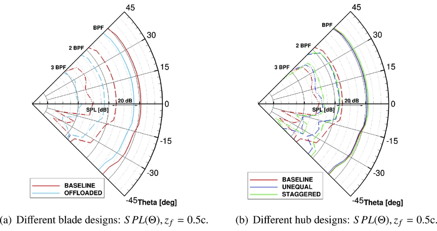
Figure 16. SPL contributions from the first three BPF tones analysis moving along the fuselage azimuth for the different IMPACTA propeller designs.
4.2.1 Cabin noise
To estimate the noise perceived by a passenger, a relation is needed that links the external pressure field to the sound pressure inside the cabin. Within the IMPACTA project, acoustic measurements were performed by NLR to experimentally determine a set of Transfer Functions (TF) describing the cabin noise response of a typical commercial aircraft(Reference Geurts73).
Tests were conducted on a Fokker 50 aircraft, inside a hangar, employing a reciprocal technique(Reference Lyamshev74) in combination with near-field acoustic holography to determine the normal particle velocity(Reference Williams75). The fuselage starboard region, where the propeller field normally impinges, was covered, for a total length of 3.10 m, extending 3/4 upstream and 1/4 downstream of the propeller rotation plane (refer to Figs 10 and 17). A linear michrophone array, mounted on a moving traversing mechanism, allowed to scan 32 × 32 points following the fuselage surface from the bottom middle line to the top, excluding the row exactly at the middle (see Fig. 10(b)). The strength of the sound source inside the cabin was measured simultaneously to the microphone data acquisitions, thus the TF contains information about both magnitude and phase. For comparing the designs, however, only the real part of the obtained pressure signal is used. Due to the monopole limitation of the uniform acoustic dodecahedron source employed, measurements were possible for frequencies between 100 Hz and 1250 Hz. Therefore, a second experiment was set up to extend the TF data to a frequency range between 57 Hz, i.e. f =
 $\frac{BPF}{2}$
, which appears in the spectra of modified hubs, and 10 kHz. At that time, a direct technique was adopted performing measurements with pure tone excitation using CFD computed signals as input for the speakers and transfer functions were determined by extrapolation. It is noted that the extrapolation method may give results of inferior accuracy than the reciprocal measurements (also because the measurements of the direct method contain the fuselage reflected field as well as the incident field) and thus introduce uncertainties; however, these results are used here for the relative evaluation of the different designs. Therefore, it is expected that these uncertainties do not significantly alter the conclusions.
$\frac{BPF}{2}$
, which appears in the spectra of modified hubs, and 10 kHz. At that time, a direct technique was adopted performing measurements with pure tone excitation using CFD computed signals as input for the speakers and transfer functions were determined by extrapolation. It is noted that the extrapolation method may give results of inferior accuracy than the reciprocal measurements (also because the measurements of the direct method contain the fuselage reflected field as well as the incident field) and thus introduce uncertainties; however, these results are used here for the relative evaluation of the different designs. Therefore, it is expected that these uncertainties do not significantly alter the conclusions.
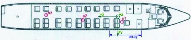
Figure 17. RNLAF Fokker 50 U-05 cabin layout and source and array positions(Reference Geurts73).
Different positions inside the cabin were considered, while the aircraft 28 seats laid out in a 2-1 configuration of Fig. 17 was kept fixed. The results presented here are representative of a passenger seated slightly ahead of the propeller plane, on the second seat away from the window (position S1 in Fig. 17). To visualise the aircraft response to the incoming pressure field, two Transmission Loss (TL) maps are presented in Fig. 18. The TL was defined as follows:
 $$\begin{equation}
TL = 20 \log _{10}\left(\frac{\vert TF \vert }{dS}\right) dB \text{,}
\end{equation}$$
$$\begin{equation}
TL = 20 \log _{10}\left(\frac{\vert TF \vert }{dS}\right) dB \text{,}
\end{equation}$$
dS being the surface covered by each microphone. As can be seen, in the transmission through the structure of the fuselage, the noise levels are reduced by more than 20 dB. The aircraft response is also shown to be non-uniform and highly dependent on the frequency of the incoming pressure field. Below 500 Hz, specific areas with low TL levels can be identified, probably in correspondence of specific structural components of the fuselage or windows. At higher frequencies, a more scattered response can be seen, with, in general, the top part of the fuselage providing a high attenuation and the bottom a reduction between 30 and 40 dB.
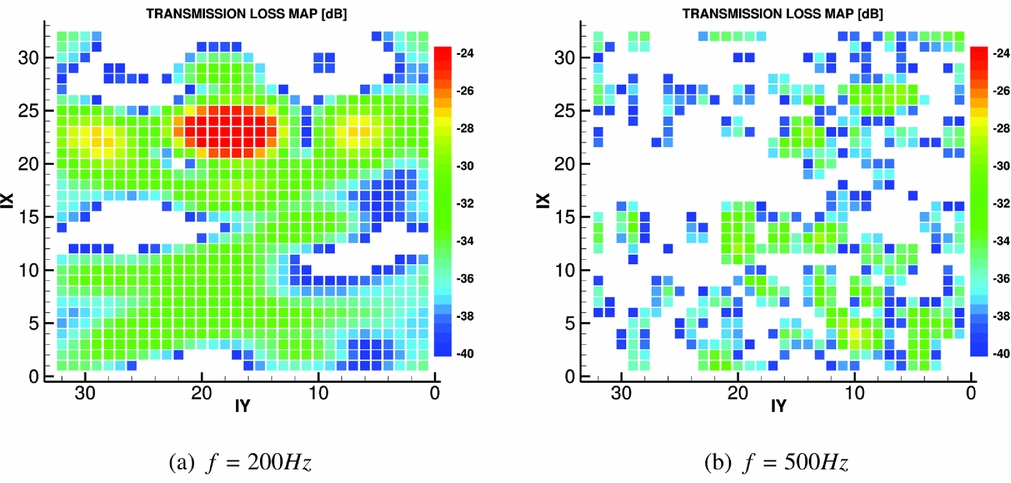
Figure 18. Transmission Loss maps: experimental measurements by NLR on a Fokker 50 aircraft(Reference Geurts73). IX and IY are the azimuthal and the longitudinal TF points indeces, starting from the lowest most forward corner of the idealised fuselage and increasing going, respectively, upstream and downstream, as shown in Fig. 10(a).
Knowing the transfer functions and given the pressure signals at the fuselage exterior, it is possible to estimate the acoustic pressure amplitude inside the cabin, and thus the pressure time history for the passenger considered. The procedure, which consists in a convolution between the pressure signals and the TF, is performed in the frequency domain via the following steps: (i) computation of the Discrete Fourier Transform of the unsteady pressure signals predicted on the fuselage external surface; (ii) multiplication of the complex Fourier coefficients from each signal by the complex TF value at the same frequency; (iii) summation of the contribution of all 32 × 32 positions; (iv) computation of the inverse Discrete Fourier Transform to have the acoustic pressure signal as function of time at the specified location inside the cabin. Some of the pressure amplitude maps (i.e.
 $\vert{\hat{p}^{\prime} (\mathbf {x},f)} \vert$
) on the external fuselage surface, and the corresponding maps inside the cabin after the TF application, are presented in Figs 19–21 for the different IMPACTA hub designs. Results are presented here using non-dimensional values based on
$\vert{\hat{p}^{\prime} (\mathbf {x},f)} \vert$
) on the external fuselage surface, and the corresponding maps inside the cabin after the TF application, are presented in Figs 19–21 for the different IMPACTA hub designs. Results are presented here using non-dimensional values based on
 $max \vert{\hat{p}^{\prime} (\mathbf{x} \text{,BPF})}\vert_{\rm Baseline}$
of the corresponding case. The magnitude of the pressure amplitude inside the cabin is considerably lower than outside. Moreover, the pressure distribution at the cabin interior differs significantly from the external one because of the non-uniform transmission characteristics of the structure of the fuselage. The energy content of the BPF tone is seen to be dominant, the 2 BPF having less than 30% and the 3 BPF having a maximum of 10% of the energy of the BPF. Because of the initial energy content combined with the high TL levels, the contribution of higher harmonics inside the cabin becomes negligible. Regarding the additional harmonics of the modified designs, only the content at f = 0.5BPF, and, to a lesser extent, the one at f = 1.5BPF, seem to be significant in the transmission through the aircraft fuselage. It is interesting to observe the different pressure distributions predicted from the Staggered hub design with respect to that from either the Baseline or the Unequally Spaced. The acoustic footprint of the two distinct rows of blades is clearly visible on the fuselage in Fig. 20.
$max \vert{\hat{p}^{\prime} (\mathbf{x} \text{,BPF})}\vert_{\rm Baseline}$
of the corresponding case. The magnitude of the pressure amplitude inside the cabin is considerably lower than outside. Moreover, the pressure distribution at the cabin interior differs significantly from the external one because of the non-uniform transmission characteristics of the structure of the fuselage. The energy content of the BPF tone is seen to be dominant, the 2 BPF having less than 30% and the 3 BPF having a maximum of 10% of the energy of the BPF. Because of the initial energy content combined with the high TL levels, the contribution of higher harmonics inside the cabin becomes negligible. Regarding the additional harmonics of the modified designs, only the content at f = 0.5BPF, and, to a lesser extent, the one at f = 1.5BPF, seem to be significant in the transmission through the aircraft fuselage. It is interesting to observe the different pressure distributions predicted from the Staggered hub design with respect to that from either the Baseline or the Unequally Spaced. The acoustic footprint of the two distinct rows of blades is clearly visible on the fuselage in Fig. 20.

Figure 19. Non-dimensional pressure fluctuations amplitude maps before (left) and after (right) the TF application: Baseline IMPACTA design. IX and IY are the azimuthal and the longitudinal TF points indeces, starting from the lowest most forward corner of the idealised fuselage and increasing going, respectively, upstream and downstream, as shown in Fig. 10(a).

Figure 20. Non-dimensional pressure fluctuations amplitude maps before (left) and after (right) the TF application: Staggered hub IMPACTA design. IX and IY are the azimuthal and the longitudinal TF points indeces, starting from the lowest most forward corner of the idealised fuselage and increasing going, respectively, upstream and downstream, as shown in Fig. 10(a).

Figure 21. Non-dimensional pressure fluctuations amplitude maps before (left) and after (right) the TF application: Unequally Spaced hub IMPACTA design. IX and IY are the azimuthal and the longitudinal TF points indeces, starting from the lowest most forward corner of the idealised fuselage and increasing, going, respectively, upstream and downstream, as shown in Fig. 10(a).
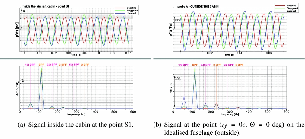
The resulting pressure signal at position S1 inside the fuselage is compared, as an example, with the one at point A on the exterior in Fig. 22. In the same figure, the spectral content of the two signals is also reported. Note that the shift in phase of the three signals is only due to the different azimuthal positions of the blades in the grid. Finally, Fig. 23 shows the sound pressure level inside the cabin and the corresponding A-weighted value. As can be seen, inside the cabin the differences between the modified hubs and the Baseline configuration are considerably reduced, but still visible.

Figure 22. Unsteady pressure signal inside (on the right) and outside (on the left) the cabin: comparison between Baseline and modified hub designs of the IMPACTA propeller.
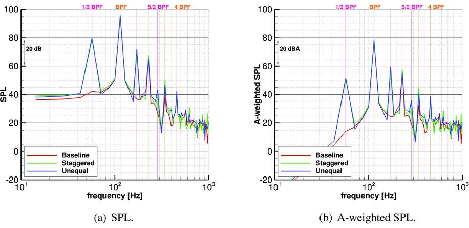
Figure 23. Sound pressure level inside the aircraft cabin at the point S1.
5.0 CONCLUDING REMARKS
The in-house CFD solver HMB3 has been validated for flows and acoustics of propellers. Subsequently, an acoustic analysis of different propeller designs in isolation (a Baseline blade, an Offloaded Tip blade, a Staggered hub and an Unequally Spaced hub) was performed using RANS simulations. OSPL and noise spectra were evaluated on an idealised high-wing aircraft fuselage and the interior cabin noise was assessed via experimental transfer functions.
The Offloaded Tip design is shown to be significantly quieter than the Baseline design because of the lower operating RPM and the load moved inboard. The Unequally Spaced hub design is shown to be slightly noisier than the Baseline design. The Staggered Hub design also yields to slightly higher noise levels, but the RPM could be further optimised. The modified hub designs exhibit a greater number of spectral peaks, leading to a spread of the acoustic energy over more frequencies. However, inside the cabin, these differences are significantly reduced and sound perception tests should be performed to evaluate if the advantages of a more continuous spectrum justify the extra manufacturing and structural complexities.
Future work will aim, on one hand, to estimate the broadband noise content using unsteady computations with lower turbulent viscosity than URANS as well as semi-empirical approaches in combination with RANS results, and on the other hand, to evaluate the propeller acoustics once installed on a turboprop aircraft. The TF will be further explored in future works where propeller installation effects are to be investigated.
ACKNOWLEDGEMENTS
This research is supported by Dowty Propellers(76). Results were obtained using the EPSRC funded ARCHIE-WeSt High Performance Computer (www.archie-west.ac.uk), that is gratefully acknowledged for the time allocated. The authors would also like to thank ARA and NLR for the use of the experimental data.