


Introduction
The rhynchonellide brachiopods, originating in the Early Ordovician, are geologically the oldest and phylogenetically most basal of the extant rhynchonelliforms (Carlson Reference Carlson2016). They survived all “big five” mass extinctions and still inhabit modern oceans (Savage et al. Reference Savage, Manceñido, Owen, Carlson, Grant, Dagys, Sun and Kaesler2002; Curry and Brunton Reference Curry, Brunton and Selden2007; Schreiber et al. Reference Schreiber, Bitner and Carlson2013, Reference Schreiber, Roopnarine and Carlson2014; Carlson Reference Carlson2016). One of the most important evolutionary changes occurred across the Permian/Triassic (P/Tr) boundary. Unlike some orders (e.g., Orthida, Productida, and Spiriferida) that went extinct during the crisis, the Rhynchonellida survived the P/Tr mass extinction and became the second most diverse order (after the Terebratulida) in the Mesozoic and Cenozoic (Lee Reference Lee2008; Carlson Reference Carlson2016); they, however, were generally a more minor component of brachiopod communities during the Paleozoic (Carlson Reference Carlson2016). When compared with the relatively better-known, cladistically based phylogenies of other orders within the Brachiopoda (Carlson Reference Carlson and Dudley1991a,Reference Carlson, MacKinnon, Lee and Campbellb, Reference Carlson1993, Reference Carlson1995; Alvarez et al. Reference Alvarez, Rong and Boucot1998; Carlson and Leighton Reference Carlson and Leighton2001; Jaecks and Carlson Reference Jaecks and Carlson2001; Carlson and Fitzgerald Reference Carlson and Fitzgerald2008; Harnik et al. Reference Harnik, Fitzgerald, Payne and Carlson2014; Congreve et al. Reference Congreve, Krug and Patzkowsky2015; Lee and Shi Reference Lee and Shi2016; Guo et al. Reference Guo, Chen and Harper2020b), the phylogenetic evolution of this successful group across the P/Tr transition still remains poorly understood. Xu (Reference Xu, MacKinnon, Lee and Campbell1990) published the first cladistic analysis of some Triassic genera, based on relatively few characters, and subsequent research confirmed that morphology-based phylogeny is a powerful tool revealing the evolution of this and other groups (Carlson Reference Carlson and Dudley1991a,Reference Carlson, MacKinnon, Lee and Campbellb, Reference Carlson1993, Reference Carlson1995; Carlson and Fitzgerald Reference Carlson and Fitzgerald2008; Congreve et al. Reference Congreve, Krug and Patzkowsky2015; Sclafani et al. Reference Sclafani, Congreve, Krug and Patzkowsky2018; Guo et al. Reference Guo, Chen and Harper2020b). Accordingly, phylogenetic analysis of Permian and Triassic rhynchonellides provides new insights into the successful evolutionary strategies of the Rhynchonellida across the P/Tr transition.
This paper aims to provide phylogenetic analyses of the late Permian to Triassic rhynchonellides at the genus level, coupled with morphologic analyses to investigate successful strategies and morphologic selectivity during their diversification following the P/Tr mass extinction. Shell size and ornamentation are two basic traits of brachiopods and other invertebrate shells that play important roles in the evolution of these animals (Payne Reference Payne2005; Vörös Reference Vörös2010; Zhang et al. Reference Zhang, Augustin and Payne2015; Schaal et al. Reference Schaal, Clapham, Rego, Wang and Payne2016; Wu et al. Reference Wu, Shi and Sun2019). Combining these characters and the trees generated, it is possible to investigate the role of heterochrony in the rhynchonellides during this critical period, which may provide useful information on the diversification dynamics of this clade (Gould Reference Gould1977; McNamara Reference McNamara2012; Schreiber et al. Reference Schreiber, Bitner and Carlson2013).
Traditionally, to reconstruct phylogenetic trees, morphologic characters are analyzed using maximum parsimony and all characters are weighted equally. Considering the homoplasy in data, some parsimony approaches that rescale characters in relation to their homoplasies have been developed (e.g., implied weighting; Goloboff Reference Goloboff1993; Goloboff et al. Reference Goloboff, Carpenter, Arias and Miranda-Esquivel2008). Recently, model-based methods, such as Bayesian analysis using the Mk model, have become increasingly popular for phylogenetic analysis and are also important approaches for evaluating biotic parallel or convergent evolution (Wagner and Marcot Reference Wagner and Marcot2010; Wagner Reference Wagner2012; Wright Reference Wright2017, Reference Wright2019). Some simulated studies have indicated that Bayesian inference provides more accurate trees than maximum parsimony (Wright and Hillis Reference Wright and Hillis2014; O'Reilly et al. Reference O'Reilly, Puttick, Parry, Tanner, Tarver, Fleming, Pisani and Donoghue2016, Reference O'Reilly, Puttick, Pisani and Donoghue2018; Puttick et al. Reference Puttick, O'Reilly, Tanner, Fleming, Clark, Holloway, Lozano-Fernandez, Parry, Tarver, Pisani and Donoghue2017, Reference Puttick, O'Reilly, Pisani and Donoghue2019), implying that this inference could be the default method for phylogenetic estimation from phenotype datasets (Puttick et al. Reference Puttick, O'Reilly, Tanner, Fleming, Clark, Holloway, Lozano-Fernandez, Parry, Tarver, Pisani and Donoghue2017). Despite many studies, the best method for phylogenetic analysis among those approaches is still not universally agreed upon (Wright and Hillis Reference Wright and Hillis2014; Congreve and Lamsdell Reference Congreve and Lamsdell2016; O'Reilly et al. Reference O'Reilly, Puttick, Parry, Tanner, Tarver, Fleming, Pisani and Donoghue2016, Reference O'Reilly, Puttick, Pisani and Donoghue2018; Puttick et al. Reference Puttick, O'Reilly, Tanner, Fleming, Clark, Holloway, Lozano-Fernandez, Parry, Tarver, Pisani and Donoghue2017, Reference Puttick, O'Reilly, Pisani and Donoghue2019; Goloboff et al. Reference Goloboff, Torres and Arias2018; Smith Reference Smith2019; Barido-Sottani et al. Reference Barido-Sottani, van Tiel, Hopkins, Wright, Stadler and Warnock2020; Keating et al. Reference Keating, Sansom, Sutton, Knight and Garwood2020; Mongiardino Koch et al. Reference Mongiardino Koch, Garwood and Parry2021).
Phylogenetic relationships and divergence times are critical for macroevolutionary studies of organisms. In the past, approaches to build time-calibrated trees involved estimating the topology and branch lengths in separate and sequential analyses (Bapst Reference Bapst2014; Bapst and Hopkins Reference Bapst and Hopkins2017). However, the temporal data of taxa include important information on the evolutionary dynamics of the group, and the traditional “node-dating” method may discard key information (Ronquist et al. Reference Ronquist, Klopfstein, Vilhelmsen, Schulmeister, Murray and Rasnitsyn2012a). By incorporating various sources of information from fossil records, the tip-dating method can deal with this problem and infer both the topology and divergence times simultaneously while accounting for their uncertainties in a coherent Bayesian statistical framework (Ronquist et al. Reference Ronquist, Klopfstein, Vilhelmsen, Schulmeister, Murray and Rasnitsyn2012a). This method has been successfully applied to many fossil groups (Bapst et al. Reference Bapst, Wright, Matzke and Lloyd2016; Matzke and Wright Reference Matzke and Wright2016; Wright Reference Wright2017; Zhang and Wang Reference Zhang and Wang2019; King and Beck Reference King and Beck2020) but has not been used for phylogenetic analysis of rhynchonellides. In addition, for analyzing morphologic and stratigraphic data simultaneously, tip-dating is an ideal tool to study the data that include the convergent evolution of taxa with temporal gaps (Lee and Yates Reference Lee and Yates2018; King and Beck Reference King and Beck2020). In the Rhynchonellida, homoplasy is common and the same external appearance can be repeated several times in the evolutionary history of the group (Ager et al. Reference Ager, Childs and Pearson1972; Cooper Reference Cooper1972; Manceñido and Owen Reference Manceñido, Owen, Brunton, Cocks and Long2001; Savage et al. Reference Savage, Manceñido, Owen, Carlson, Grant, Dagys, Sun and Kaesler2002). Therefore, in this study, tip-dated Bayesian (TB) analysis is employed to reconstruct phylogenetic trees for the late Permian and Triassic rhynchonellides. To investigate the effect of tip-dating on tree topology, the same data are also analyzed using other methods: equal-weighting parsimony (EW), implied-weighting parsimony (IW), and undated Bayesian (UB).
Data and Methods
Occurrence and Duration Data
The occurrence data and stratigraphic ranges of genera were downloaded from the Paleobiology Database (paleobiodb.org). Some doubtful records were amended or excluded. The generic durations based on original descriptive papers and recently published monographs were revised (Shen et al. Reference Shen, Jin, Zhang, Weldon, Rong, Jin, Shen and Zhan2017; Sun et al. Reference Sun, Xu, Qiao, Rong, Jin, Shen and Zhan2017). Some newly established genera, not included in Treatise on Invertebrate Paleontology were also added. In the following analysis, the stage bin was used for time intervals. When a genus occurred before and after a stage in the actual fossil record, then it was also assumed to be present within that stage.
Taxon Selection and Character Coding
Taxon Selection
Unlike higher-level phylogenetic analyses that usually involve a restricted number of taxa in each family/subfamily, the genus-level analysis includes more lower-rank morphologic variation and also helps test the reality and integrity of family-level groups. For late Permian rhynchonellides, the superfamily Lambdarinoidea is unique in both its external and internal characters when compared with other more “normal” rhynchonellides. Only one species of this superfamily was reported from the upper Permian (Grant Reference Grant1988; Baliński and Sun Reference Baliński and Sun2008); this superfamily therefore is excluded from the present analysis.
Previous studies have shown that a small number of characters selected from a large number of taxa may generate poorly resolved consensus trees (Puttick et al. Reference Puttick, O'Reilly, Tanner, Fleming, Clark, Holloway, Lozano-Fernandez, Parry, Tarver, Pisani and Donoghue2017; O'Reilly and Donoghue Reference O'Reilly and Donoghue2018; Schrago et al. Reference Schrago, Aguiar and Mello2018; Barido-Sottani et al. Reference Barido-Sottani, van Tiel, Hopkins, Wright, Stadler and Warnock2020). In addition, computation time may be greatly increased if too many taxa are included. Therefore, the genera whose internal characters (especially the crura, which is a very important structure in traditional classification of this group) are not well known were excluded from the present analyses. Coledium was also deleted, because the species (Coledium erugatum) that perfectly confirms the diagnosis of this genus occurs in the lower Carboniferous and has a large time gap between itself and other coded taxa. The Griesbachian (early Induan) genus Meishanorhynchia is one of the earliest representatives of Mesozoic-type rhynchonellides and is crucial in understanding the initial recovery of this clade after the P/Tr mass extinction, but the anterior parts of its crura remain poorly defined (Chen et al. Reference Chen, Shi and Kaiho2002). However, some newly obtained material from the type locality (in Meishan, eastern China) of the type species of Meishanorhynchia reveals that its crura are laterally compressed and almost straight anteriorly, typical of spinuliforms (Supplementary Fig. S1; see also Supplementary Text). A total of 71 genera (including Meishanorhynchia) were coded for analysis. The type species of most genera were coded based on original and updated taxonomic descriptions. Where some important characters are unknown in the type species, a well-described species that has the same generic affiliation was selected. The list of genera coded and uncoded is provided in the Supplementary Material.
Characters
The morphologic terms follow Williams et al. (Reference Williams, Brunton, MacKinnon and Kaesler1997) and Savage et al. (Reference Savage, Manceñido, Owen, Carlson, Grant, Dagys, Sun and Kaesler2002). Fifty-seven discrete characters were employed in the analysis (Supplementary Data). Of these, 24 characters describe the external appearance of shells, including outline, sulcus and fold, valve convexity, ornamentation, ventral umbo, pedicle opening, and stolidium. The remaining 33 are associated with internal structures and shell perforations; seven of them are related to crura. Characters could be binary or multistate and were treated as unordered in the analysis. Most characters adopted here are comparable with those used by Schreiber et al. (Reference Schreiber, Bitner and Carlson2013). However, some characters used in Schreiber et al. (Reference Schreiber, Bitner and Carlson2013) are not adopted in the present analysis. This is because the latter study is focused on living species, and some characters (e.g., sizes of muscle scars, shapes of teeth, development of socket ridges) can be observed directly from living shells, but these characters may not be observed in fossilized brachiopods whose internal structures are usually reconstructed by a means of serial sections.
Tip-dated Bayesian Inference Analyses
Ages of tips are very important information in these analyses, and the stratigraphic interval of each tip must therefore be determined before the analyses. Here we employed two approaches: “species-dating” and “genus-dating” to calibrate the tips (see Supplementary Data for tip dates used in this study), and the morphologic character data were analyzed using both approaches. In the first approach, a tip was dated based on stratigraphic occurrences of selected species from which the morphologic data were derived. For instance, the characters of Abrekia were summarized based on those of its type species Abrekia sulcata described by Dagys (Reference Dagys1974) from the Induan in the Russian Far East region, and the tip date of Abrekia therefore is 251.9 to 251.2 Ma, the occurrence range of A. sulcata. This method has the highest levels of accuracy and precision in estimating divergence times (Püschel et al. Reference Püschel, O'Reilly, Pisani and Donoghue2020), although this is not the main goal of our study. In the second tip-calibration approach, the species of a genus were assumed to have the same character states. The age of a tip was given based on the first geologic stage in the range of a genus, and the Wuchiapingian was treated as the tip date of late Permian taxa. For example, Abrekia has a range from the Induan to the Anisian, and it first appeared in the Induan; its tip age is therefore given as 251.9 to 251.2 Ma. Tip ages of a taxon are sometimes identical for these two methods (e.g., Abrekia), but they can be different as well. In both approaches, tip ages were assigned uniform priors over the range of uncertainty (Barido-Sottani et al. Reference Barido-Sottani, Aguirre-Fernández, Hopkins, Stadler and Warnock2019, Reference Barido-Sottani, van Tiel, Hopkins, Wright, Stadler and Warnock2020).
TB analysis was performed using BEAST v. 2.6.2 (Bouckaert et al. Reference Bouckaert, Vaughan, Barido-Sottani, Duchêne, Fourment, Gavryushkina, Heled, Jones, Kuhnert, De Maio, Matschiner, Mendes, Müller, Ogilvie, du Plessis, Popinga, Rambaut, Rasmussen, Siveroni, Suchard, Wu, Xie, Zhang, Stadler and Drummond2019). The Mk model (Lewis Reference Lewis2001) was used, with a gamma distribution to account for rate variation across sites. Characters were partitioned according to the number of character states. The clock model was an uncorrelated lognormal clock (Drummond et al. Reference Drummond, Ho, Phillips and Rambaut2006), and the tree prior was a sampled-ancestor fossilized birth–death model (Gavryushkina et al. Reference Gavryushkina, Welch, Stadler and Drummond2014). Because the evolutionary history of the rhynchonellide brachiopods is poorly studied, the parameters thus varied within a relatively wide range; the distributions of parameters are listed in Supplementary Text. The analysis was run for 800 million generations, sampling every 200,000, saving 4001 trees. The first 50% of trees (2000 trees) were discarded as burn-in to ensure that the chains had reached a stationary condition. Convergence of four independent runs was assessed based on effective sample size values >200 and confirmed in Tracer v. 1.7 (Rambaut et al. Reference Rambaut, Drummond, Xie, Baele and Suchard2018) and the R package RWTY (Warren et al. Reference Warren, Geneva and Lanfear2017). The default maximum clade credibility (MCC) consensus tree method was applied to summarize the posterior sample of trees (there are four runs and 2001 trees are retained for every run, so the posterior sample has 8004 trees). Additionally, another consensus tree method, the 50% majority-rule consensus (MRC) tree was also deployed, using PAUP* v. 4.0a166 (Swofford Reference Swofford2003). Previous studies showed that the MCC tree is probably not a good method to summarize the results of Bayesian phylogenetic analyses of morphologic data, because it often includes more incorrect clades than the MRC tree (O'Reilly and Donoghue Reference O'Reilly and Donoghue2018). However, although the MRC tree has higher accuracy, it is usually poorly resolved (especially for small datasets like ours; Puttick et al. Reference Puttick, O'Reilly, Tanner, Fleming, Clark, Holloway, Lozano-Fernandez, Parry, Tarver, Pisani and Donoghue2017; Schrago et al. Reference Schrago, Aguiar and Mello2018), and it is almost impossible to capture much useful information if there are substantial polytomies that cannot be used in the character analysis. The fully resolved MCC tree has more incorrect nodes than the MRC tree, but at the same time, it possibly contains more correct nodes (O'Reilly and Donoghue Reference O'Reilly and Donoghue2018). In this study, many nodes recovered by the MCC tree are not well supported (see “Results”). To avoid utilizing the MCC tree as the only input in the following analysis, multiple posterior trees were also analyzed to account for the uncertainty of the tree topology and divergence times (Wright et al. Reference Wright, Lyons, Brandley and Hillis2015, Reference Wright, Wagner and Wright2021; Bapst et al. Reference Bapst, Wright, Matzke and Lloyd2016; Soul and Wright Reference Soul and Wright2021).
Lineage Richness
Although the trees generated by TB include information on branch lengths and divergence times, every taxon is considered as a point occurrence in time, and therefore, the trees do not display the stratigraphic range of the taxa (Bapst et al. Reference Bapst, Wright, Matzke and Lloyd2016). Also, during the analyses, the presence of mass extinction was not considered, and many Triassic lineages were dated back to the Permian (Supplementary Fig. S5). Previous studies on empirical datasets have shown that the tip-calibrated analyses tend to inaccurately recover old divergence-time estimates, and the dating approaches can affect the results of downstream analyses (Ronquist et al. Reference Ronquist, Klopfstein, Vilhelmsen, Schulmeister, Murray and Rasnitsyn2012a, Reference Ronquist, Lartillot and Phillips2016; Bapst Reference Bapst2014; O'Reilly et al. Reference O'Reilly, Dos Reis and Donoghue2015; Bapst et al. Reference Bapst, Wright, Matzke and Lloyd2016; Matzke and Wright Reference Matzke and Wright2016; Bapst and Hopkins Reference Bapst and Hopkins2017; Püschel et al. Reference Püschel, O'Reilly, Pisani and Donoghue2020; Simões et al. Reference Simões, Caldwell and Pierce2020). Therefore, to calculate lineage richness over time, we adopted the topology of the tip-dated trees and recalibrated them using the cal3 method (Bapst Reference Bapst2013) in the R package paleotree (Bapst Reference Bapst2012). This approach uses the probabilistic model of branching, extinction, and sampling processes to date samples of trees, and it stochastically draws divergence dates given a set of rates for those processes (Bapst Reference Bapst2013). Simulation studies imply that the cal3 method performs better than other posterior time-scaling methods (Bapst Reference Bapst2014; Bapst and Hopkins Reference Bapst and Hopkins2017). The three rates (branching, extinction, and sampling rates) needed in cal3 were calculated based on the BEAST2 posterior estimates, and their median values were selected. The time ranges of genera are in discrete stratigraphic intervals; therefore, the function bin_cal3TimePaleoPhy was used, and the first and last appearance dates of each taxon were placed within their first and last intervals under a uniform distribution. This method was applied to both species-dated and genus-dated trees, although the values input for the three rates for species-dated trees may be less accurate, as tip ages in the species-dated analysis are not identical to the first appearance of genera. One thousand dating replicates were performed for each of the two MCC trees, respectively, and one median curve for each tree was calculated. In addition, we also calculated lineage richness for all the posterior samples of trees (8004 trees) generated under both the tip-calibration methods (species-dating and genus-dating). Every tree was calibrated once, and all 8004 curves were plotted on the same figure.
Character Analysis
Shell Size
The shape of the rhynchonellide shell was approximated as an ellipsoid, so the formula 4π × 3−1 × (0.5L) × (0.5W) × (0.5T) was applied to calculate the shell volume of each genus, where L is the shell length, W the width, and T the thickness. For each coded species, the largest specimen in the original or emended descriptions was measured. Then, the shell volume data were normalized by log 10 transformation (Supplementary Data).
Ornamentation
The development of ornamentation was evaluated by the ornamentation index (OI). The product of “ornamentation length,” “ornamentation coarseness,” and “ornamentation strength” was used to describe the OI. The ornamentation length describes the distribution of ribs. A rib having a full length was given a value of 1, while a smooth shell was given a value of 0. A rib arising slightly anterior to the umbo, beginning at midlength, and confined to the anterior margin was given values of 0.8, 0.5, and 0.2, respectively. Ribs confined to the sulcus were coded as 0.5. The ornamentation coarseness is measured and coded as follows: coarse and fine plicae (number of ribs <20) possess a value of 1, and very fine ribs (number of ribs >20) are coded as 0.5. Antidichotomous ribs (fine costae that merge anteriorly to form coarse plicae) were treated as coarse plicae, and only the anteriorly coarse part was considered in the OI calculation. The ornamentation strength has three values: 0, 0.5, and 1, which represent absent, faint (e.g., Cyrolexis), and distinct ornamentation (e.g., Rhynchonelloidea), respectively. The OI values therefore range from 0 to 1 (Supplementary Data). To sum up, the longer, coarser, and stronger ribs have the greater OI values, and when ribs are absent, the OI value is 0. Although the OI has discrete values, it was treated as a continuous character in this analysis.
Evolutionary Trend of Shell Size and OI in Fossil Record
To investigate the evolutionary trends of size and OI, we calculated shell size and OI values for all genera from the upper Permian and Triassic based on their type species. Variations in these values were calculated for each stage from the late Permian to Triassic based on their durations from fossil records; the structures of trees are not considered in this analysis. For shell size, the Mann-Whitney test was applied to evaluate whether there is a significant change in shell size between two adjacent stages. The variation of ornamentation development was represented by the mean of the OI.
Ancestral-State Estimation
To investigate the distribution and evolution of size and OI on phylogenetic trees, ancestral-state reconstruction was performed using the fastAnc function in the R package phytools (Revell Reference Revell2012), which generates maximum-likelihood ancestral states assuming a Brownian motion model. The reconstructed ancestral states were plotted on the MCC trees using the contMap function. Moreover, we paid special attention to the character evolution of the Early and early Middle Triassic “small-sized taxa” (see “Results”). We compared the character states of the tips (i.e., the small-sized taxa) and those of their ancestral nodes. The most recent ancestral node of a tip was labeled as “AN1,” and the most recent ancestral node of AN1 was termed “AN2,” and so on. In total, character states of four groups of ancestral nodes (AN1 to AN4) were considered. As mentioned earlier, the branch length or the tree topology may affect the comparative analysis, and we conducted this analysis for both BEAST2-generated (not recalibrated) trees and cal3-recalibrated trees. For both cases, a thousand (1000) trees were randomly sampled from the posterior sample of trees, and the recovered character states of AN1–AN4 of the 1000 trees were recorded and displayed in box plots. In a very small number of trees, some genera do not have AN4 and/or AN3, and the states of those nodes were not considered. All calculations were performed using R (R Core Team 2020).
Phylogenetic Analyses Using Other Methods
Out-Group
In addition to tip-dated analyses, the same data were also analyzed using EW, IW, and UB. For these analyses, a camerelloid genus, Camerella was chosen as the out-group (Schreiber et al. Reference Schreiber, Bitner and Carlson2013). The Camerelloidea belongs to the Pentamerida, but that superfamily was closely allied to the Rhynchonellida (Carlson et al. Reference Carlson, Boucot, Rong and Blodgett2002; Schreiber et al. Reference Schreiber, Bitner and Carlson2013). Instead of the type species, another species, Camerella bella, was selected to be coded to represent Camerella following Schreiber et al. (Reference Schreiber, Bitner and Carlson2013).
IW and EW Analyses
IW can down-weight characters according to their homoplasy. The extent of down-weighting under IW is controlled by a concavity constant (k) (Farris Reference Farris1969; Goloboff Reference Goloboff1993). A very low k-value strongly penalizes the homoplastic characters, and IW begins to exhibit the undesirable properties of clique analysis. Nevertheless, when a k-value is very high, IW performs like EW (Goloboff et al. Reference Goloboff, Carpenter, Arias and Miranda-Esquivel2008, Reference Goloboff, Torres and Arias2018; Smith Reference Smith2019). In the present analysis, we applied the TNT script setk.run, written by Salvador Arias, to search for the appropriate value of k. The script returned a value of k = 12.63 of our data; that value was adopted in IW.
Parsimony analyses were performed using TNT v. 1.5 (Goloboff and Catalano Reference Goloboff and Catalano2016). For both EW and IW, heuristic searches were performed using traditional search algorithms. Ten thousand replicates were executed, saving 10 trees per replicate. The strict consensus trees were calculated for the most parsimonious trees (MPTs). Bootstrap values were calculated to examine the results of EW analysis, and symmetric resampling support values were calculated for the IW analysis.
UB Analysis
UB analysis was performed in MrBayes v. 3.2.6 (Huelsenbeck and Ronquist Reference Huelsenbeck and Ronquist2001; Ronquist and Huelsenbeck Reference Ronquist and Huelsenbeck2003; Ronquist et al. Reference Ronquist, Teslenko, van der Mark, Ayres, Darling, Höhna, Larget, Liu, Suchard and Huelsenbeck2012b). The Mk model (Lewis Reference Lewis2001) with gamma distribution priors for site rate variation was used for analysis. The prior on the gamma shape parameter was a uniform distribution between 0 and 10. The analysis was run for 80 million generations with four runs of four chains that sampled every 20,000. Convergence of the four runs was confirmed in Tracer v. 1.7 (Rambaut et al. Reference Rambaut, Drummond, Xie, Baele and Suchard2018) and standard deviation of split frequencies <0.01. The first 50% of trees were discarded as burn-in. The 50% MRC tree was constructed for the posterior sample of trees using the sumt function in MrBayes. Moreover, the MCC tree was also calculated using TreeAnnotator in BEAST v. 2.6.2 (Bouckaert et al. Reference Bouckaert, Vaughan, Barido-Sottani, Duchêne, Fourment, Gavryushkina, Heled, Jones, Kuhnert, De Maio, Matschiner, Mendes, Müller, Ogilvie, du Plessis, Popinga, Rambaut, Rasmussen, Siveroni, Suchard, Wu, Xie, Zhang, Stadler and Drummond2019). All consensus trees and the character–taxon matrix in Nexus format are provided in the Supplementary Material.
Results
Tree Topology
Tip-dated Bayesian Inference Analyses
For both calibration approaches, the 50% MRC trees are poorly resolved, as expected (Supplementary Fig. S2). Therefore, only the MCC trees are displayed here (Fig. 1). When tips are calibrated using the species-dating method, the members of the Paleozoic superfamily Stenoscismatoidea form a clade in the basal part of the tree (Fig. 1A). Other Paleozoic taxa and the Triassic genus Lissorhynchia are included in a monophyletic group, which is a sister group of the clade consisting of other Mesozoic taxa. In the larger Mesozoic group (from Homoeorhynchia to Caucasorhynchella), taxa are classified as two poorly supported clades. The smaller clade includes halorellids, wellerelloids, pugnacoids, some norelloids, and two raduliform genera: Caucasorhynchella and Aorhynchia. Although their crural types and superfamilial affiliations are variable (see Supplementary Data), they all lack developed septal plates and a dorsal septalium. Except halorellids and the two raduliform genera, all other members in this clade are grouped into three subclades: the Batongorhynchia–Laevirhynchia clade, which has weak ornamentation and lacks dental plates; the Austriellula–Trigonirhynchella clade, which features weak dental plates and weak ornamentation; and the Calcirhynchia–Veghirhychia clade, which is characterized by fully and densely costate shells. The other large monophyletic group in this tree consists of the raduliform (or variations thereof) genera and the Dimerellidae. Most of the genera in this group have developed dental plates, septal plates, and a dorsal septalium. Some monophyletic groups are also recognized in the tree, but many of them are not strongly supported.
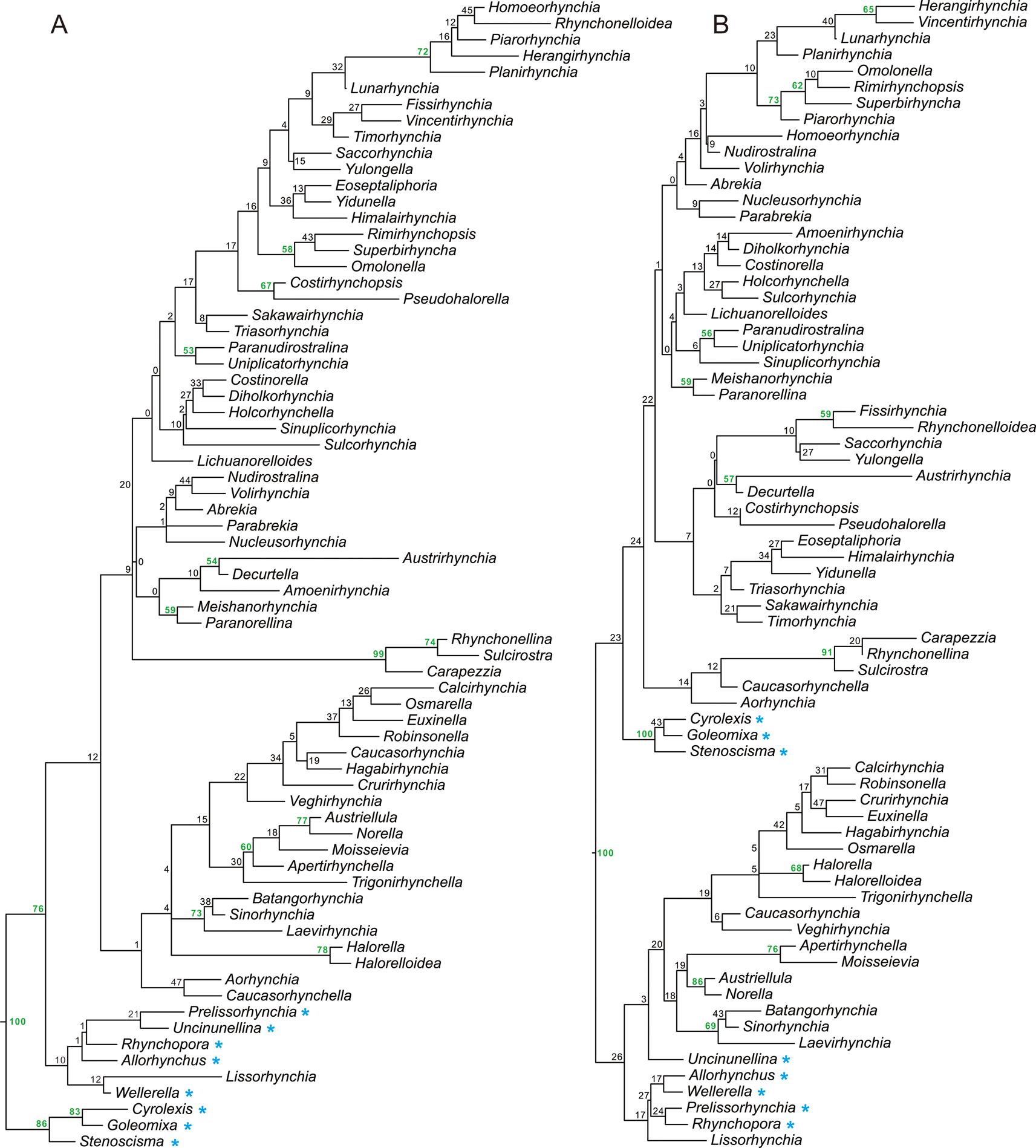
Figure 1. Maximum clade credibility (MCC) trees generated by “species-dated” (A) and “genus-dated” (B) analyses. The posterior probability of each clade is presented as a node label (as percentage). Values over 50 are in bold. Paleozoic genera are marked by asterisks.
The MCC tree generated using the genus-dating method displays two large clades (Fig. 1B). The lower one consists of wellerelloids, pugnacoids, some norelloids, and members of Halorellidae. Some Paleozoic members grouped in this clade are located in its basal parts. Some members of the Norelloidea (Norella, Austriellula, Batangothynchia, and Laevirhynchia) are grouped in a monophyletic group, together with three wellerelloid genera: Sinorhynchia, Apertirhynchella, and Moisseievia. The other large clade includes members of the Stenoscismatoidea, Dimerellidae, Rhynchonelloidea, Hemithiridoidea, and Rhynchotetradoidea, and some norelloids also appear in this group. Except for the Stenoscismatoidea, which is located in basal positions, three smaller clades are classified: the Carapezzia–Aorhynchia clade, which has variable internal structure and ornamentation; the Fissirhynchia–Timorhynchia clade, which is characterized by an entirely costate shell; and the Herangirhynchia–Paranorellina clade, which has a partially costate shell.
Other Analytical Methods
Consensus trees generated using the EW, IW, and UB are provided in the Supplementary Material. In all these trees (Supplementary Figs. S3, S4), the Stenoscismatoidea forms a clade in the basal part of the tree. Nevertheless, in contrast to the tip-dated MCC trees discussed earlier, many Paleozoic members are located in relatively derived positions. Raduliform (or variations thereof) genera are often reconstructed as paraphyletic associations (they are included in a monophyletic group in the MCC tree generated by UB; Supplementary Fig. S4), and the septifal and arcuiform members are included in a monophyletic group. Although topologies are different among these trees and many nodes are not strongly supported, the general pattern of taxonomic and character distributions is highly comparable: raduliform (or variations thereof) genera in the lower part, members of the Dimerelloidea (sensu Savage et al. Reference Savage, Manceñido, Owen, Carlson, Grant, Dagys, Sun and Kaesler2002) in the middle part, and septifal or arcuiform elements in the upper part.
Lineage Richness Variation
Generic richness of fossil data underwent a dramatic drop across the P/Tr boundary (Fig. 2A) and remained rather low during the Early Triassic (Induan–Olenekian). The Anisian (early Middle Triassic) saw the first increase in generic richness of Triassic rhynchonellides, with the number of genera exceeding pre-extinction levels. Then, generic richness experienced a gentle decline in the Ladinian, followed by a stepwise increase through the Ladinian to the Norian, with a pronounced peak in the Norian.
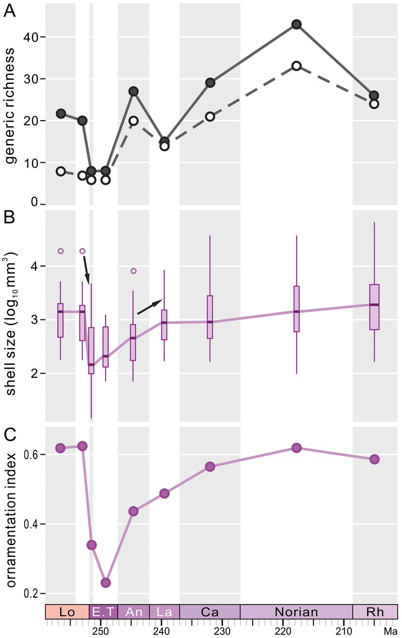
Figure 2. A, Numbers of genera in each stage from the upper Permian to Triassic. Black dot indicates the number of genera recorded in that bin, and open circle indicates taxa included in our phylogenetic analysis. B, Box plot of shell size through time. Open circles are outliers, and a solid line indicates variation of the median value. An arrow is labeled when the change of shell size between the two adjacent stages is significant (p < 0.05). C, Mean of ornamentation index (OI). These curves are based on fossil data, and phylogenetic structures are not considered. Lo, Lopingian; E.T, Early Triassic; An, Anisian; La, Ladinian; Ca, Carnian; Rh, Rhaetian.
The lineage diversities calculated based on the two MCC trees are shown in Supplementary Figure S5. Both curves show a gradual increase in lineage richness from the late middle Permian to the early Middle Triassic, although there are some minor fluctuations, and a small drop in lineage richness occurred in the late Permian on the curve based on the genus-dated MCC tree. From the Middle Triassic to the end of the Triassic, the lineage richness varied strongly, and there are several obvious losses and increases in lineage diversity.
The lineage richness calculated using raw tip-dated MCC trees does not consider the last appearances of genera. By contrast, the stratigraphic ranges were added by recalibrating trees using the cal3 method. The lineage richnesses calculated by cal3-calibrated trees are displayed in Figure 3. Although the trees generated using these two calibration approaches (genus-dated and species-dated) are not mutually consistent in topology, the lineage richness variations calculated based on these two methods are very close to one another (Fig. 3). In addition, the general trends of lineage richness outlined by posterior tree samples (8004 trees) and by MCC trees are comparable. Lineage richness derived from those two approaches shows no evident loss across the P/Tr boundary, which is expected, as many Changhsingian genera that disappeared in the P/Tr extinction, were not included in phylogenetic analyses. Instead, a pronounced increase in lineage richness occurred from the Early Triassic to the Anisian. Also, richness in the Anisian almost reached the highest level seen in the Triassic. After the Anisian, the richness in both lineages fluctuated slightly and maintained a high level until the middle Norian. The lineage richness, coupled with generic richness, declined markedly in the Rhaetian (Fig. 3).
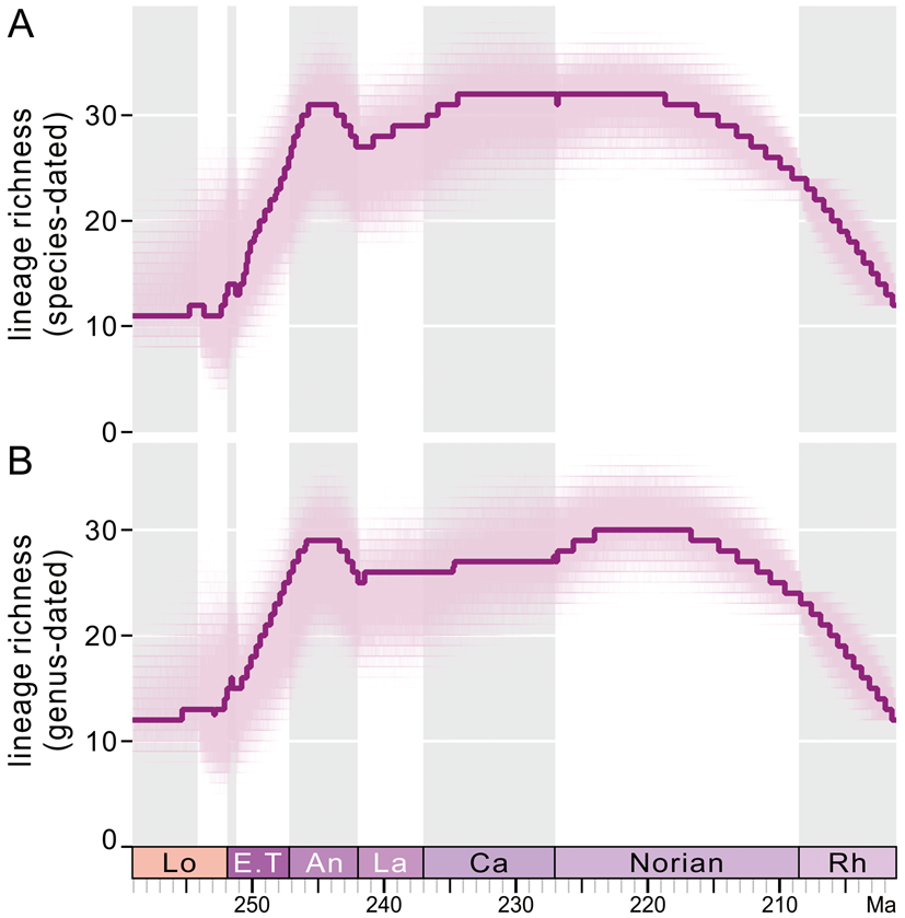
Figure 3. Lineage diversity calculated from cal3-recalibrated posterior samples of trees and maximum clade credibility (MCC) trees based on the “species-dated” method (A) and “genus-dated” method (B). Solid lines represent median diversities calculated from 1000 recalibrated MCC trees. In both A and B, the light clouds are composed of 8004 curves that are generated by recalibrations of 8004 trees of posterior samples; every tree was recalibrated once. Lo, Lopingian; E.T, Early Triassic; An, Anisian; La, Ladinian; Ca, Carnian; Rh, Rhaetian.
Shell Size Variation
Fossil records show that rhynchonellide shell sizes suffered a conspicuous reduction across the P/Tr boundary and reached their lowest values in the Induan (Fig. 2B). The rather low levels of body sizes through the Induan to Olenekian within the Early Triassic interval indicate the miniaturization of rhynchonellide brachiopods in the aftermath of the P/Tr extinction. Then, body sizes increased significantly in the Anisian, followed by a gentle, stepwise increase through the Middle–Late Triassic, but never returned to pre-extinction levels until the Norian (Fig. 2B).
After an estimation of ancestral states, shell sizes and the OI values are plotted on the MCC trees generated by TB analysis (Figs. 4, 5, Supplementary Figs. S6–S9). In both species-dated and genus-dated trees, there are some small-sized elements in the aftermath of the P/Tr extinction, and most are in the upper parts of the figures, such as Meishanorhynchia, Paranorellina, Nucleusorhynchia, Abrekia, Parabrekia, and Lichuanorelloides. They are not within a monophyletic group, but all appear to have close relationships with some members of the Rhynchonelloidea (sensu Savage et al. Reference Savage, Manceñido, Owen, Carlson, Grant, Dagys, Sun and Kaesler2002). In the following discussion, they are termed “small-sized taxa.” Their ancestral nodes usually have a darker color (i.e., larger size) than the small-sized taxa (see Fig. 4), suggesting that the small-sized shell is a derived state. Moreover, there are some taxa of distinctly larger size: Sulcirostra, Rhynchonellina, Carapezzia, Halorella, and Halorelloidea (“large-sized taxa” in the following discussion). These taxa belong to the Dimerelloidea (Dimerellidae and Halorellidae; sensu Savage et al. Reference Savage, Manceñido, Owen, Carlson, Grant, Dagys, Sun and Kaesler2002), but the latter is not a monophyletic group according to our results. In some parts of the trees, the descendant lineages seem to have larger shell sizes than their parent lineages. Although there are several exceptions, both the Homoeorhynchia–Paranorellina clade in the species-dated MCC tree and the Herangirhynchia–Paranorellina clade in the genus-dated MCC tree display an increasing trend in shell size along the lineages (Fig. 4, Supplementary Figs. S6, S7).
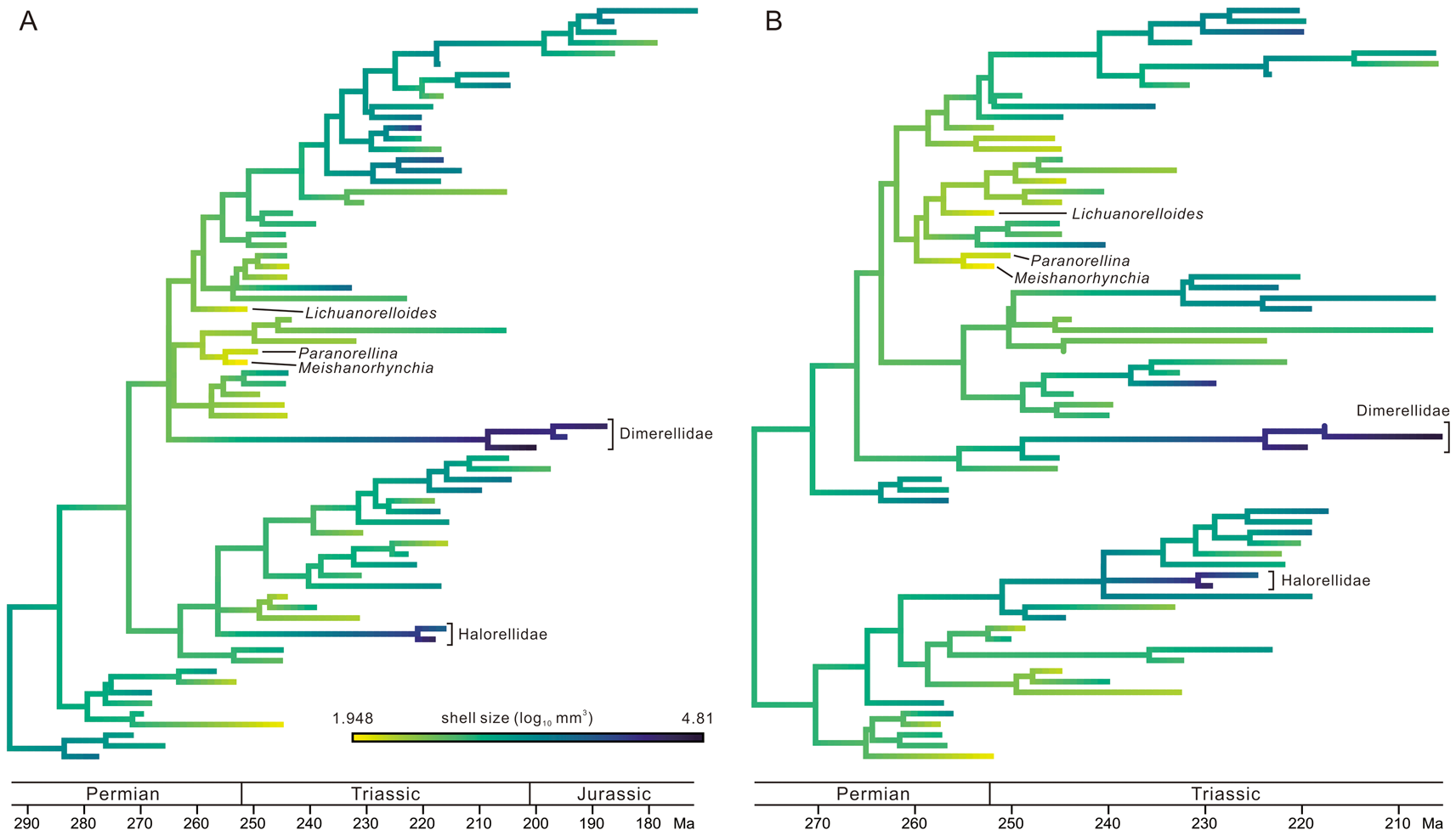
Figure 4. Ancestral-state reconstruction of shell size, plotted on the “species-dated” maximum clade credibility (MCC) tree (A) and the “genus-dated” MCC tree (B). Darker color means larger size (online version in color). See Supplementary Material for the same figure with all taxa labeled.

Figure 5. Ancestral-state reconstruction of ornamentation index (OI), plotted on the “species-dated” maximum clade credibility (MCC) tree (A) and the “genus-dated” MCC tree (B). Darker color means higher OI and more pronounced ornamentation (online version in color). See Supplementary Material for the same figure with all taxa labeled.
The character states of the ancestral nodes of the small-sized taxa were estimated across 1000 trees randomly selected from the posterior samples. The analytical results for genus-dated trees and species-dated trees (Fig. 6, Supplementary Fig. S10A,B) are almost identical to one another, so only the former is shown here. For all six genera, there is a downward trend in shell size from the AN4s to the tips in both tip-dated trees and recalibrated trees, and it is more obvious in the three Early Triassic genera Meishanorhynchia, Lichuanorelloides, and Paranorellina. The only exceptions are that in some cases, the sizes of Paranorellina and Abrekia are slightly larger than the median sizes of their respective AN1 and/or AN2.
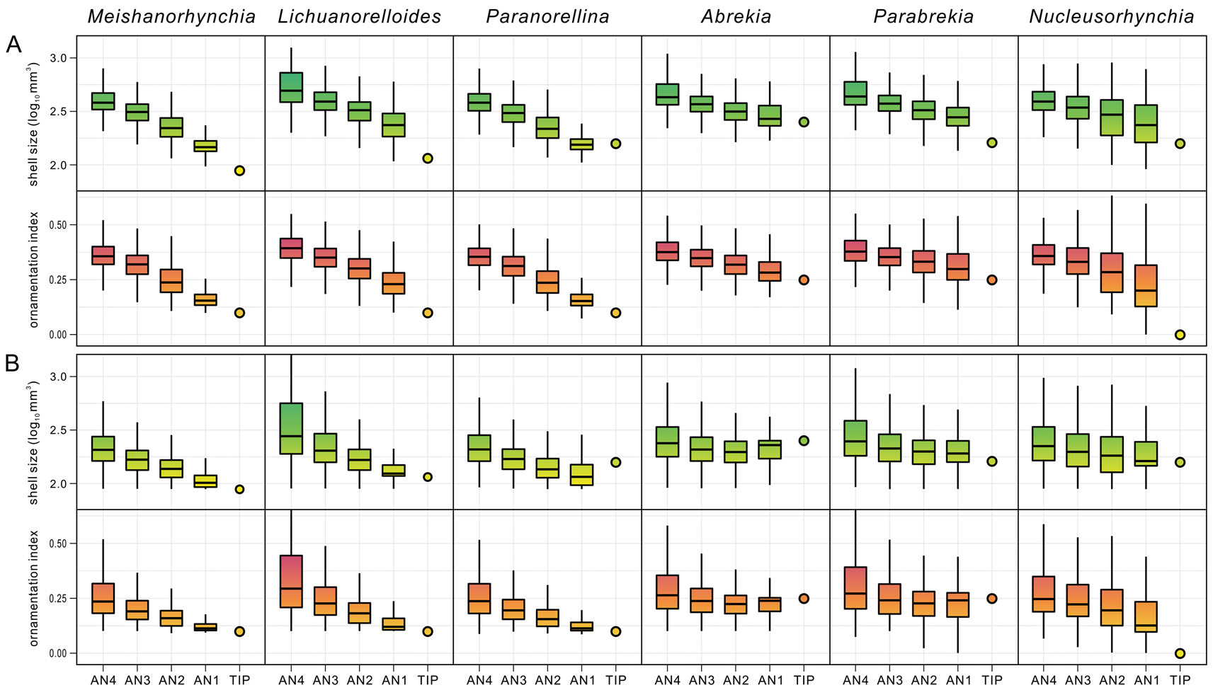
Figure 6. Estimates of character states of the “small-sized taxa” (tips) and their respective ancestral nodes (AN1–AN4) based on 1000 trees randomly selected from the posterior samples. A, Results calculated from non-recalibrated “genus-dated” trees. B, Results calculated from cal3-recalibrated “genus-dated” trees. Outliers are omitted.
Ornamentation Variation
The OI measures the development of ornamentation on shells. Clearly, the OI values also experienced a dramatic decline across the P/Tr boundary (Fig. 2C). This decline continued from the Induan to the Olenekian (Early Triassic). The same proxy increased rapidly in the Anisian, followed by a gentle, stepwise increase in the Middle–Late Triassic. The postextinction OI values eventually reached pre-extinction levels in the Late Triassic.
In our dataset, two large groups of taxa have the most prominent ornamentation: fully costate and raduliform elements (mostly hemithiridoids) and fully costate and septifal taxa (mostly wellerelloids and pungnacoids). In addition, there are two weakly ornamented groups: the semicostate and raduliform taxa (roughly equal to the small-sized taxa) and the smooth or slightly ribbed arcuiform and septifal genera (e.g., Norella, Austriellula, Batangorhynchia, Laevirhynchia, Sinorhynchia, and Trigonirhynchella). In the two MCC trees, neither increase nor decrease in OI is obvious in the “arcuiform and septifal groups,” but a trend of increasing OI is possibly present in the “semicostate and raduliform group” (Fig. 5, Supplementary Figs. S8, S9): the Early to Middle Triassic small-sized taxa have the weakest ornamentation within the semicostate group, and the later diversified clades have relatively higher OI values. As for shell size, the ancestral nodes of the small-sized taxa also have a darker color, indicating their ancestors may have had more developed costae (Fig. 5, Supplementary Figs. S8, S9). Similarly, the estimates of the states of their ancestral nodes across multiple trees exhibit a decreasing trend in OI from the AN4s to the tips as well (Fig. 6, Supplementary Fig. S10A,B), and again, this trend is rather prominent in Meishanorhynchia, Lichuanorelloides, and Paranorellina.
Discussion
Analytical Methods and Tree Topology
Traditionally, morphologic data are analyzed using parsimony methods. To diminish the effect of homoplasy, the IW approach was introduced (Goloboff Reference Goloboff1993; Goloboff et al. Reference Goloboff, Carpenter, Arias and Miranda-Esquivel2008). For our dataset, the external characters exhibit substantial homoplasy, and therefore, they were down-weighted more under IW. Several nodes in the consensus trees clearly indicate the effect of IW (Supplementary Fig. S3). For example, in the EW strict consensus tree, Laevirhynchia is grouped with Uniplicatorhynchia, because they are very similar in external appearance such as having smooth shells and a uniplicate commissure. Nevertheless, their internal characters are very different. Unlike Uniplicatorhynchia, Laevirhynchia lacks dental plates and a septalium and shows a closer relationship with Batangorhynchia and Sinorhynchia in the IW tree. The latter two genera also lack dental plates and a septalium. The 50% MRC tree generated by UB is poorly resolved (Supplementary Fig. S4). Even so, general patterns of taxa and character distribution in this tree are also comparable with those demonstrated in the IW and EW consensus trees, as stated earlier. Also, many clades in the MCC tree generated by UB are identical with those of the EW and IW consensus trees. Therefore, although topologies are not completely identical, trees generated using the three methods: EW, IW, and UB are broadly similar (King Reference King2020).
By incorporating stratigraphic information into phylogenetic analysis, TB generates quite different trees from the other three methods, and tip-dated MCC trees obviously have better stratigraphic congruence (King Reference King2020). In tip-dated MCC trees (Fig. 1), all the Paleozoic taxa are positioned in the basal part; nevertheless, many of them (mostly wellerelloids) are reconstructed in derived positions in EW, IW, and UB consensus trees (Supplementary Figs. S2–S4). This discordance of topology and stratigraphic position can be caused by a variety of factors (Carlson and Fitzgerald Reference Carlson and Fitzgerald2008). Intuitively, it is possible that the choice of out-group determines the position of those wellerelloids. The out-group taxon Camerella has external ornamentation and crura similar to those of the stenoscismatoids and Triassic semicostate rhynchonelloids. Consequently, these taxa are grouped in the basal part of the tree, and the wellerelloids, having very different characters from Camerella, migrated to relatively derived positions in the trees. Also, the earliest members of this group are not included in this study, and character states of the Triassic rhynchonellides may have appeared many times in the long history of this order. In this case, the choice of out-group will be challenging. TB, which does not need an out-group taxon, is more appropriate for the analysis of our data.
Although the IW method can lessen the effect of homoplasy, it does not consider the temporal disparity between taxa. If two species with a large stratigraphic gap develop very similar characters independently (convergent evolution), they will be grouped together in IW trees (e.g., the Late Triassic Himalairhynchia and the Paleozoic Rhynchopora; Supplementary Fig. S3). In contrast, taking account of the temporal gap between these two species, they are positioned in two mutually remote clades in the tip-dated trees (Fig. 1). Thus, for such groups as rhynchonellides, which have a limited number of characters and sometimes display homoplasy, our study indicates that TB maybe a better method than EW, IW, and UB to reconstruct the phylogenetic relationships. In this study, the evolutionary relationships of the rhynchonellides displayed in tip-dated MCC trees are much closer to their actual stratigraphic occurrences in the fossil record, and thus the relationships are more reliable, if we assume that the fossil records of this group are relatively complete and dependable.
However, this advantage of TB may also generate questionable relationships if the fossil records are incomplete. For instance, if two closely related species are discovered from two horizons with a large temporal gap and no comparable fossils are reported in this gap, the tree generated using TB may mistakenly place them in two different clades, especially when the character signal is weak (King Reference King2020). This can be reflected by trees generated by two different calibration approaches. In the genus-dated MCC tree, Nudirostralina and Homoeorhynchia are closely located (tip dates: Nudirostralina, Olenekian; Homoeorhynchia, Carnian), as well as in the EW, IW, and UB consensus trees (Fig. 1B, Supplementary Figs. S3, S4). However, in the species-dated MCC tree (Fig. 1A), they are far apart from one another, which is possibly caused by the large temporal gap between the coded species of the two genera (tip dates: Nudirostralina, Anisian; Homoeorhynchia, Pliensbachian). Another example is the different position of Norella. It has a long range from the Olenekian to the Rhaetian. In the species-dated tree (Fig. 1A), however, it was positioned in a relatively derived position, because its tip age was given as “Norian” in that analysis. The differences in topology between the genus-dated and species-dated MCC trees indicate that for some taxa, character signals can be overturned by temporal signals (King Reference King2020). Because the temporal gaps between genera are generally smaller in genus-dated analysis when compared with those used in species-dated analysis, character signals played relatively more important roles in the former. Therefore, the MCC tree generated by the genus-dated method is closer to traditional classifications that are proposed according to characters.
It is noticeable that in all the consensus trees (Fig. 1, Supplementary Figs. S3, S4), many nodes are not strongly supported. This is caused by the limitations of this morphologic dataset, which includes many genera with limited numbers of characters and character states, thus, it is difficult to generate consistent topologies for Bayesian or bootstrap analyses. As stated in “Data and Methods,” the MCC tree is not a recommended method to summarize a posterior sample of trees (O'Reilly and Donoghue Reference O'Reilly and Donoghue2018). However, the MCC tree is a tree with the greatest production of clade probabilities, and at least, it represents one of the most credible tree structures; moreover, it provides more valuable information than the MRC tree if the latter recovers rare nodes and clades. The low posterior support of nodes (i.e., highly variable topology) is not uncommon in empirical datasets (O'Reilly and Donoghue Reference O'Reilly and Donoghue2018; Barido-Sottani et al. Reference Barido-Sottani, van Tiel, Hopkins, Wright, Stadler and Warnock2020), and the tree topology and divergence times affect the results of phylogenetic comparative analysis (Bapst Reference Bapst2014; Bapst and Hopkins Reference Bapst and Hopkins2017). However, the downstream comparative analyses are not impossible if multiple trees, rather than a single point estimate of phylogeny, are analyzed (Wright et al. Reference Wright, Lyons, Brandley and Hillis2015; Bapst et al. Reference Bapst, Wright, Matzke and Lloyd2016; Soul and Wright Reference Soul and Wright2021).
Lineage Evolution of the P-Tr Rhynchonellides
The stratigraphic ranges of genera were treated differently in the raw tip-dated MCC tree and recalibrated trees (the last appearances were not considered in the former analysis). Thus, the lineage richness in the late Middle to Late Triassic cannot be compared directly, because many taxa that originated in the early Middle Triassic and persisted to the Late Triassic were not counted in the curves based on raw MCC trees. However, an outstanding discrepancy occurs between the “raw” and “recalibrated” lineage richness on the left parts of the curves. In the raw MCC trees, many nodes were dated back to the middle and late Permian, resulting in an increase in lineage richness at that time. By contrast, the nodes recalibrated by the cal3 method seem to have a relatively younger age, thus, the lineage diversity increased frequently in the Early and Middle Triassic. Considering that the P/Tr extinction is the most severe extinction event in Earth's history (Chen and Benton Reference Chen and Benton2012), many Paleozoic lineages were likely truncated across the P/Tr boundary, and most Triassic lineages diversified after the extinction. If this is true, the richness calculated by the cal3 method is more reliable. The tendency of tip-calibrated analyses to recover inaccurately old divergence-time estimates (or “deep root attraction”) has been observed in many datasets (Ronquist et al. Reference Ronquist, Klopfstein, Vilhelmsen, Schulmeister, Murray and Rasnitsyn2012a, Reference Ronquist, Lartillot and Phillips2016; O'Reilly et al. Reference O'Reilly, Dos Reis and Donoghue2015; Bapst et al. Reference Bapst, Wright, Matzke and Lloyd2016; Matzke and Wright Reference Matzke and Wright2016; Püschel et al. Reference Püschel, O'Reilly, Pisani and Donoghue2020; Simões et al. Reference Simões, Caldwell and Pierce2020). Many factors may have caused the deep root attraction, such as an inadequate model of morphologic evolution and the prior distributions of the parameters (Ronquist et al. Reference Ronquist, Klopfstein, Vilhelmsen, Schulmeister, Murray and Rasnitsyn2012a, Reference Ronquist, Lartillot and Phillips2016; Püschel et al. Reference Püschel, O'Reilly, Pisani and Donoghue2020). Maybe more sophisticated models or carefully constrained values of parameters are needed to deal with it (Ronquist et al. Reference Ronquist, Lartillot and Phillips2016; Simões et al. Reference Simões, Caldwell and Pierce2020).
All the calculated lineage richnesses show an evident increase in the Early and early Middle Triassic and reach the highest level in Anisian. In contrast, generic diversity peaked in the Norian. The lineage diversification of the rhynchonellides in the Early and early Middle Triassic is partially consistent with taxonomic diversification in fossil records. The small-sized taxa appeared early in the ocean after the P/Tr mass extinction (Chen et al. Reference Chen, Shi and Kaiho2002, Reference Chen, Kaiho and George2005a, Reference Chen, Kaiho and Georgeb, Reference Chen, Tong, Kaiho and Kawahata2007; Wang et al. Reference Wang, Chen, Dai and Song2017; Wu et al. Reference Wu, Zhang and Sun2021), and they represent the earliest Mesozoic-type rhynchonellides. In the Olenekian, in addition to the raduliform (or variations thereof) genera, there are other newly originated genera such as the arcuiform Norella and Lissorhynchia. The Anisian also witnessed a great biodiversification of rhynchonellides (Yang and Xu Reference Yang and Xu1966; Dagys Reference Dagys1974; Pálfy Reference Pálfy2003; Chen et al. Reference Chen, Kaiho and George2005a, Reference Chen, Zhao, Wang, Luo and Guo2018; Guo et al. Reference Guo, Chen and Harper2020a). The Anisian taxa developed a variety of external and internal structures, for example, smooth or semicostate or fully costate shells, possession or lack of dental plates, a septalium and dorsal median septum, and occurrences of various types of crura. Many higher-level classification units in the traditional classification schemes therefore have already appeared in the Anisian. All these data indicate that the diversity and morphologic complexity of rhynchonellides recovered in the Anisian and even exceeded the pre-extinction levels.
Moreover, lineage richness of cal3-calibrated trees decreased gradually from the late Norian to the Rhaetian probably due to the “Signor-Lipps effect” (Signor and Lipps Reference Signor and Lipps1982; Wagner Reference Wagner2019). Because the last appearances of genera are uniformly distributed through their last stratigraphic intervals, generic extinctions occur before the end-Rhaetian and gradually increase in frequency toward the Triassic/Jurassic boundary, resulting in a gradual loss in lineage richness. Similarly, the diversification in the Early and early Middle Triassic also may be biased by the “Jaanusson effect” (i.e., the first appearances of genera may be younger than their true origin time, making the pattern of very rapid diversification appear to be gradual; Jaanusson Reference Jaanusson and Bassett1976) to some extent, which usually delays the recovery of diversity. Regardless, these results indicate that the lineage richness reached almost the highest level before the end-Anisian.
It is noteworthy that we used the relatively simple fossilized birth–death model in this study. However, it is highly possible that the evolutionary dynamics of the rhynchonellides differ during the extinction, radiation, and background intervals. Therefore, further efforts based on more complicated models (such as the skyline model; Stadler et al. Reference Stadler, Kühnert, Bonhoeffer and Drummond2013; Gavryushkina et al. Reference Gavryushkina, Welch, Stadler and Drummond2014) and informative priors should be made in the future (Simões et al. Reference Simões, Caldwell and Pierce2020; Wright et al. Reference Wright, Wagner and Wright2021). Stratigraphic range data of taxa may also be retained in analyses with the uncertainties of ages considered (Stadler et al. Reference Stadler, Gavryushkina, Warnock, Drummond and Heath2018; Barido-Sottani et al. Reference Barido-Sottani, Aguirre-Fernández, Hopkins, Stadler and Warnock2019, Reference Barido-Sottani, van Tiel, Hopkins, Wright, Stadler and Warnock2020). If the divergence times are properly estimated, there will be no need to recalibrate trees using posterior approaches, which is the original goal of this method.
Shell Size and Ornamentation Evolutions
Shell size was not included in the phylogenetic analysis, and its distribution on trees therefore is not predicted by the tree topology. As stated earlier, some genera are conspicuous in all consensus trees in terms of shell sizes (Fig. 4, Supplementary Figs. S6, S7). Of these, the large-sized brachiopods belong to the Dimerelloidea (sensu Savage et al. Reference Savage, Manceñido, Owen, Carlson, Grant, Dagys, Sun and Kaesler2002); they are not a monophyletic group on our trees. These taxa are unusual and were thought to have inhabited hydrocarbon seeps and hydrothermal vents (Campbell and Bottjer Reference Campbell and Bottjer1995; Peckmann et al. Reference Peckmann, Campbell, Walliser and Reitner2007, Reference Peckmann, Kiel, Sandy, Taylor and Goedert2011, Reference Peckmann, Sandy, Taylor, Gier and Bach2013; Sandy Reference Sandy and Kiel2010; Kiel et al. Reference Kiel, Glodny, Birgel, Bulot, Campbell, Gaillard, Graziano, Kaim, Lazǎr, Sandy and Peckmann2014). The specialized hydrothermal habitats offered sufficient nutrients for dimerelloids to grow large (Kiel et al. Reference Kiel, Glodny, Birgel, Bulot, Campbell, Gaillard, Graziano, Kaim, Lazǎr, Sandy and Peckmann2014). The apparent miniaturization of shell size in Early Triassic was accentuated by the disappearance of the large Permian genera and the diversification of small-sized individuals (Fig. 4). Some parts of the MCC trees also show the increasing shell sizes along lineages, as noted in the “Results” (Fig. 4, Supplementary Figs. S6, S7), but the mechanism of enlargement is poorly understood.
With respect to the variation of ornamentation, a sharp drop in OI coincided with the P/Tr extinction (Fig. 2C). Within the Early Triassic, most of the newly originated elements (e.g., Abrekia, Laevorhynchia, Lichuanorelloides, and Meishanorhynchia) have smooth or semicostate shells that are lower in OI compared with fully costate genera, which resulted in the low OI value in the Early Triassic. The reason why the Induan saw a slightly higher OI than that in the Olenekian is that a Permian fully ribbed taxon (Terebratuloidea) temporarily survived the P/Tr extinction (Chen et al. Reference Chen, Tong, Zhang, Yang, Liao, Song and Chen2009) and increased the mean OI of the Induan. For some completely smooth or costate groups, closely related taxa may have very different ornamentation (e.g., ribbed Halorella vs. smooth Halorelloidea, capillate Rhynchonellina vs. ribbed Sulcirosta; Fig. 5); the development of ornamentation does not correlate significantly with shell size. For semicostate groups, however, it is suggested that the development of ornamentation varies during ontogeny, with larger individuals often having longer and more prominent plications than smaller ones (Cooper and Grant Reference Cooper and Grant1976; Wang et al. Reference Wang, Chen, Dai and Song2017; Fig. 7). This is also observed on our trees: the variations of shell size and OI of the superfamily Rhynchonelloidea and its affinities are highly mutually consistent (Figs. 4, 5). Brachiopod ornamentation is thought to have prevented predation (Leighton Reference Leighton1999; Vörös Reference Vörös2010). Strong external sculpture is an important protective mechanism for Mesozoic brachiopods, and the escalation of predators was also reflected by the increased ornamentation of brachiopod clades during the Mesozoic marine revolution (Vörös Reference Vörös2010). However, considering the different patterns of ornamentation development in various clades, more detailed studies are needed to investigate the relationships between OI and predation pressure.
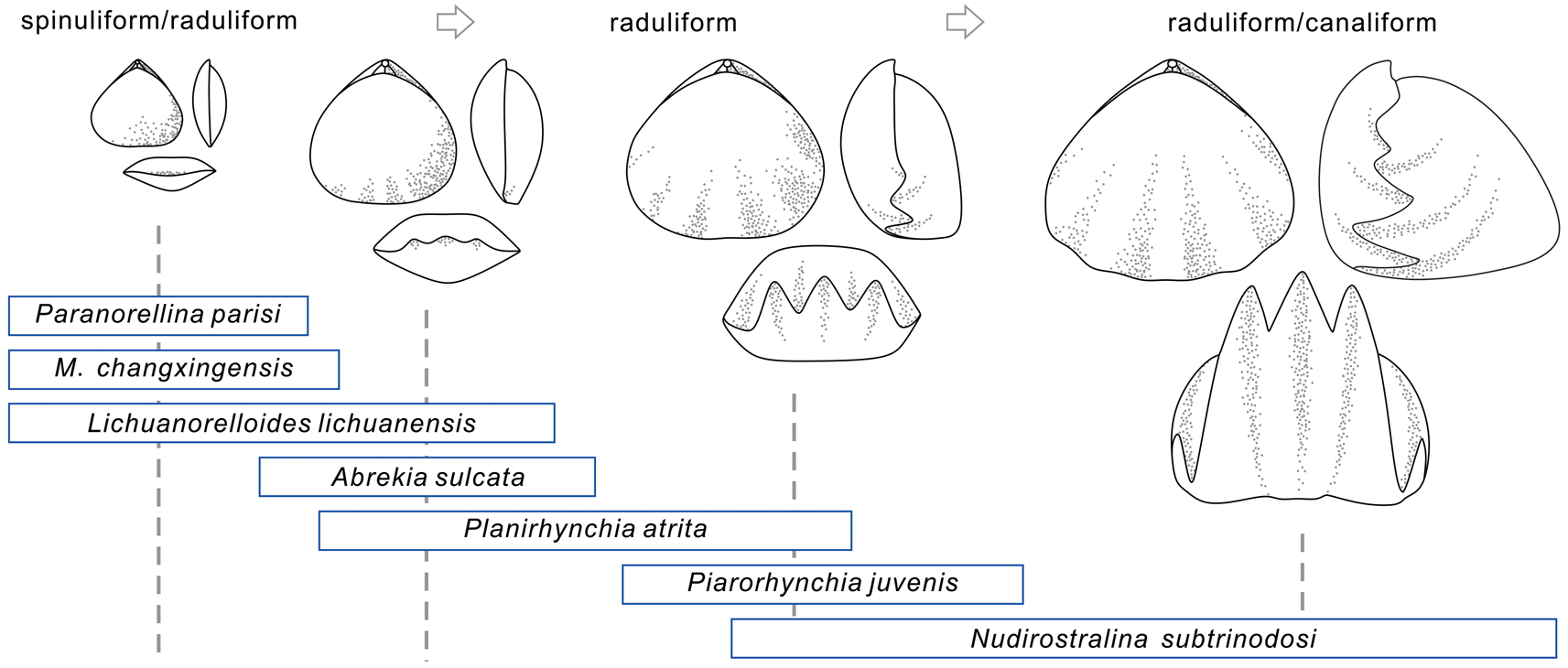
Figure 7. Possible ontogeny of members or close relatives of the Rhynchonelloidea. Some species are listed here, and the rectangular shape indicates ontogenetic stages observed in the fossil record (Ager Reference Ager1962; Dagys Reference Dagys1968, Reference Dagys1974; Chen et al. Reference Chen, Shi and Kaiho2002; Wang et al. Reference Wang, Chen, Dai and Song2017; Guo et al. Reference Guo, Chen and Harper2020a). Note that not every species undergoes all these developmental stages. M., Meishanorhynchia.
Paedomorphosis in the Small-sized Taxa
Paedomorphosis is a pattern of heterochrony wherein growth is retarded during ontogeny in descendants, compared with their ancestors, and is common among extinct and extant animals, including brachiopods (Gould Reference Gould1977; MacKinnon Reference MacKinnon, Brunton, Cocks and Long2001; McNamara Reference McNamara2012; Bitner et al. Reference Bitner, Melnik and Zezina2013). The occurrence of the small and smooth Meishanorhynchia in the aftermath of the P/Tr extinction was assumed to be an example of paedomorphosis because of its small size and spinuliform crura (Manceñido and Motchurova-Dekova Reference Manceñido and Motchurova-Dekova2010). In fact, in addition to Meishanorhynchia, other small-sized taxa are also possibly paedomorphic taxa. These taxa were traditionally assigned to two superfamilies: the Rhynchonelloidea and Norelloidea. Our analysis does not support a monophyletic group, but they appear to be closely related to some members of the Rhynchonelloidea (sensu Savage et al. Reference Savage, Manceñido, Owen, Carlson, Grant, Dagys, Sun and Kaesler2002). As members or close relatives of the Rhynchonelloidea, the small-sized taxa display a smaller size and weaker ornamentation compared with larger relatives. The estimated ancestral states show that in general, the ancestors of the small-sized taxa have a relatively larger size and more pronounced ornamentation than their descendants, with these features being more prominent in the Induan Meishanorhynchia and Lichuanorelloides (Figs. 4–6). As mentioned earlier, Paranorellina may have slightly larger size than its AN1. This is because it is always recovered as a sister taxon of Meishanorhynchia, which has a smaller size than Paranorellina, but appeared earlier than the latter. The estimated size of their AN1 (they have the same AN1) therefore is closer to that of Meishanorhynchia and smaller than that of Paranorellina. In addition to a small size and weak ornamentation, all these taxa have a depressed profile, a low fold and shallow sulcus, low convexity, and spinuliform to incipiently raduliform crura, which are often regarded as features of the juveniles of some strongly convex rhynchonellide genera (Ager Reference Ager1962; Dagys Reference Dagys1968; Wang et al. Reference Wang, Chen, Dai and Song2017; Fig. 7). These characters, together with the reconstructed ancestral states for shell size and OI, imply paedomorphic origins for the small-sized taxa among the Triassic rhynchonellides.
Paedomorphosis is induced by progenesis, postdisplacement, and neoteny (McKinney and McNamara Reference McKinney and McNamara1991; McNamara Reference McNamara2012). Any one of these processes or their combinations can result in paedomorphosis. Usually, only when life histories of taxa are well known and compared, can a specific cause be detected (McKinney and McNamara Reference McKinney and McNamara1991; Jaecks and Carlson Reference Jaecks and Carlson2001). Nevertheless, for many fossil taxa such as rhynchonellide brachiopods, it is not easy to judge which process has played the most important role in the formation of the heterochronic pattern due to the incompleteness of fossil preservation. Paedomorphosis can be stimulated by many extrinsic factors, for example, temperature, predation pressure, habitats, and nutrient supply (McNamara Reference McNamara1983; McKinney and McNamara Reference McKinney and McNamara1991). Meishanorhynchia appeared rapidly in the aftermath of the P/Tr extinction (Chen et al. Reference Chen, Shi and Kaiho2002, Reference Chen, Tong, Kaiho and Kawahata2007), and other small-sized taxa were already diverse in the Early and Middle Triassic. Accumulating evidence shows that some harmful factors, such as high seawater temperature, limited nutrition, low oxygen content, and microbial bloom associated with the P/Tr extinction, recurred in Early Triassic oceans (Erwin Reference Erwin2006; Knoll et al. Reference Knoll, Bambach, Payne, Pruss and Fischer2007; Chen and Benton Reference Chen and Benton2012; Sun et al. Reference Sun, Joachimski, Wignall, Yan, Chen, Jiang, Wang and Lai2012; Song et al. Reference Song, Wignall, Chu, Tong, Sun, Song, He and Tian2014; Chen et al. Reference Chen, Yang, Luo, Benton, Kaiho, Zhao, Huang, Zhang, Fang, Jiang, Qiu, Li, Tu, Shi, Zhang, Feng and Chen2015, Reference Chen, Tu, Pei, Ogg, Fang, Wu, Feng, Huang, Guo and Yang2019; Huang et al. Reference Huang, Chen, Wignall and Zhao2017, Reference Huang, Chen, Algeo, Zhao, Baud, Bhat, Zhang and Guo2019). For rhynchonellide brachiopods, lack of food, low oxygen, and low carbonate saturation in seawater may limit their ability to produce calcium carbonate to form shell substance, resulting in small-sized shells with weak ornamentation. To survive and develop in the inhospitable, unstable, and unpredictable environment of the Early Triassic, it is possible that these animals had to mature rapidly to reproduce and shorten their life spans, essentially in “r-selection” mode (Reznick et al. Reference Reznick, Bryant and Bashey2002). These processes also indicate that progenesis is probably the primary trigger of paedomorphosis in this group. More confident conclusions are possible if their “ancestors” are more fully sampled, and their life history can be more completely studied.
Conclusion
Phylogenetic analysis of the late Permian to Triassic rhynchonellide brachiopods was performed with four methods: EW, IW, UB, and TB. The results indicate that analytical methods have a significant effect on the topology of trees and any following analysis based on these trees. Compared with trees generated by EW, IW, and UB in which Permian and Triassic taxa are mixed together, tip-dated trees appear to be more reasonable and the revealed evolutionary relationships more consistent with the fossil record. Although the topology and branch lengths vary greatly among trees generated by different analytical approaches (species-dating vs. genus-dating, tip-dating vs. posterior rescaling), the downstream analyses based on multiple posterior trees generate some comparable results. According to the cal3-calibrated trees, the major increase in lineage richness occurred in the Early and early Middle Triassic and reached its highest level in the Anisian. The Anisian taxa evolved complex and diverse internal and external characters, implying the full recovery of this order. Both shell size and the strength of ornamentation diminished rapidly after the P/Tr extinction. The decline in these two measures was likely caused by the disappearance of larger and sculptured Permian genera and the radiation of minute and weakly ornamented taxa. Ancestral-state estimations of shell size and the development of ornamentation, along with comparisons of other characters, show that the Early to Middle Triassic small-sized taxa probably have characters displayed by juveniles of their ancestors, implying that paedomorphosis was a likely survival strategy that developed in the adverse environments after the P/Tr extinction.
In this study, we provide a preliminary tip-dated analysis for the late Permian and Triassic rhynchonellides using the relatively simple fossilized birth–death model. However, further efforts based on more complicated models and informative priors will be a key future line of enquiry. In addition, further paleontological studies on the Early Triassic rhynchonellides are needed to develop more persuasive conclusions for the paedomorphosis of the small-sized taxa. Directly sampling their ancestors and studying their ontogenies will provide tests for these hypotheses.
Acknowledgments
We sincerely thank A. M. Popov, B. Radulović, M. Siblík, and X. Guo for their help procuring some publications. We are very grateful to S. Arias for sharing his TNT script. T. L. Stubbs and M. J. Benton are acknowledged for helpful guidance on the analytical approaches. We thank M. Clapham, three anonymous reviewers, and associate editor J. Crampton for their critical comments and constructive suggestions that have improved greatly the quality of this paper. The contributors of the Paleobiology Database are also thanked for their provision of the taxonomic data for the database. This study was supported by three NSFC grants (41821001, 41930322, and 41772007), 111 Project of China (grant no. BP0820004), and the Fundamental Research Funds for National Universities, China University of Geosciences (Wuhan). This is a contribution to the IGCP 630: “Permian–Triassic Climatic and Environmental Extremes and Biotic Responses.”
Data Availability Statement
Data available from the Dryad Digital Repository: https://doi.org/10.5061/dryad.b5mkkwhdm.
Supplementary Text Contents: (1) List of genera that are not included in analyses. (2) Serial sections of Meishanorhynchia. (3) Characters applied in phylogenetic analyses. (4) Distributions and values of parameters for tip-dated analysis. (5) Other consensus trees generated by phylogenetic analyses. (6) Supplementary Figures S1–S10.
Supplementary Data Contents: (1) Character-taxon matrix and tip dates for phylogenetic analyses. (2) Shell size and OI of analyzed rhynchonellides. (3) Crural types of coded genera. (4) Familial and superfamilial attribution of analyzed taxa (based on Treatise on Invertebrate Paleontology; Savage et al. Reference Savage, Manceñido, Owen, Carlson, Grant, Dagys, Sun and Kaesler2002; Manceñido et al. Reference Manceñido, Owen, Sun and Selden2007).
Other Supplementary Files: Character-taxon matrix and consensus trees in Nexus format.


