


1. Introduction
A basic question arises about a practical method for simulating wall-bounded turbulent flow: Can a hybrid turbulence model – in the present case, detached eddy simulation – plausibly capture laminar-to-turbulent transition? The answer is far from obvious. Indeed, for many hybrid models, the answer is no. However, for solution adaptive models, it is a viable question and warrants enquiry.
In a direct numerical simulation of transition, a great deal of expense goes into capturing the very small scales of motion that are created by the breakdown mechanism. Often these are of less interest than the transition location, skin friction profile and other gross properties. So the challenge to hybrid simulation is to avoid small scales, and to capture the larger features of transition. The fundamental question is whether one can emulate transition without fully simulating the detailed breakdown mechanism.
Solution adaptation allows hybrid models to revert to laminar flow prior to transition; that occurs automatically, by suppressing the turbulent viscosity. Then the initial instabilities of a laminar boundary layer can be simulated. As these disturbances grow and start to break down, adaptivity causes the model to activate. In doing so, the eddy viscosity increases and damps the small-scale features, while the Reynolds-averaged Navier–Stokes (RANS) model adds Reynolds stresses. This is a fundamentally hybrid description. It contrasts with wall-resolved large eddy simulations (LES) of transition, in which small-scale features must be captured (Ham et al. Reference Ham, Lien, Wu, Wang and Durbin2000; Lardeau, Leschziner & Zaki Reference Lardeau, Leschziner and Zaki2012).
Hence, transition is a combination of resolving large-scale low-frequency precursors to transition, then activating the model as the flow starts to become turbulent. Activating a model is not the same as simulating transition mechanisms; but, if the adaptive method activates the model at the same location that transition would occur, it provides a prospect for applying hybrid simulation to transitional flows.
Laminar-to-turbulent transition can occur through several routes: orderly, bypass, separation-induced and shear layer impingement (Durbin Reference Durbin2017). Orderly transition usually starts with two-dimensional (2-D) Tollmien–Schlichting (TS) waves with spatially growing amplitudes. The TS waves develop three-dimensional (3-D) perturbations after they reach a certain critical amplitude. The 3-D disturbances develop into  $\Lambda$ vortices, which lift away from the wall. This is where nonlinear breakdown leads to sparse turbulent spots. The turbulent spots grow denser and larger, increase in frequency and merge to form the fully turbulent boundary layer.
Bypass transition usually happens under free-stream turbulence with an intensity of approximately 1 % or more. The boundary layer transitions from laminar to fully turbulent flow without the occurrence of TS waves, hence the term ‘bypass’. The precursors to transition are large-amplitude elongated streaks, termed Klebanoff modes. These streaks are created by low-frequency perturbations that penetrate from the free stream into the boundary layer, while transition is triggered by high-frequency non-penetrating disturbances interacting with the jet-like disturbances when they lift up to the upper part of the boundary layer (Zaki & Durbin Reference Zaki and Durbin2005).
The detached eddy simulation (DES) was first proposed in Spalart (Reference Spalart1997) as a hybrid RANS/LES method to solve the attached boundary layer using a Reynolds-averaged closure model and to resolve eddies where massive separation occurs. The formulation is straightforward: an upper limit is applied to the RANS length scale in a dissipation term. When the limiter is active, dissipation is enhanced, which reduces eddy viscosity, and allows large turbulent eddies to be resolved.
The initial formulation of DES suffers from some defects. The delayed detached eddy simulation (DDES; Spalart et al. Reference Spalart, Deck, Shur, Squires, Strelets and Travin2006) was introduced to overcome them. DDES shields the near-wall RANS region to prevent premature grid-induced separation. Later, the improved delayed detached eddy simulation (IDDES) was introduced so that DES could emulate wall-modelled LES, in which the nearly RANS region serves as a wall model. These developments are reviewed in Spalart (Reference Spalart2009).
An alternative formulation, the  $\ell ^2$–
 $\omega$ DDES model, was developed by Reddy, Ryon & Durbin (Reference Reddy, Ryon and Durbin2014) for the purpose of switching directly to subgrid viscosity, without relaxation in transport equations, and for mimicking the Smagorinsky subgrid viscosity in eddy-resolving regions. In this case, the length scale occurs in the production term of the
  $k$-equation.
These DES models contain a coefficient,  $C_{DES}$, in the length-scale limiter. In the original DES, DDES and IDDES, its value is a global constant. To allow the subgrid model to respond to the local flow, an adaptive procedure to compute
  $C_{DES}$ was developed for the
  $\ell ^2$–
 $\omega$ model (Yin, Reddy & Durbin Reference Yin, Reddy and Durbin2015; Yin & Durbin Reference Yin and Durbin2016). It was found that
  $C_{DES}$ determines not only the subgrid viscosity, but also the thickness of the shielded region. Careful formulation of the length-scale limiting function allows the adaptive DES model to achieve wall-resolved eddy simulation if the mesh resolution is adequate (Yin & Durbin Reference Yin and Durbin2016). The ability of the model to adjust to the mesh is why this is called ‘adaptive’.
In laminar regions, the dynamic evaluation of  $C_{DES}$ causes the subgrid model to vanish. This and the ability of adaptive DES to perform wall-resolved eddy simulation inspires an interest in using it to predict laminar-to-turbulent transition. Yin & Durbin (Reference Yin and Durbin2016) contains an initial assessment of transition capability for orderly (H-type and K-type), bypass and separation-induced transition. The adaptive
  $\ell ^2$–
 $\omega$ model was found to capture some of the transition mechanisms on particular meshes.
Efforts to apply hybrid RANS/LES methods to laminar-to-turbulent transition have previously been made by Walters & Cokljat (Reference Walters and Cokljat2008), Sørensen, Bechmann & Zahle (Reference Sørensen, Bechmann and Zahle2011), Alam, Walters & Thompson (Reference Alam, Walters and Thompson2013), Hodara & Smith (Reference Hodara and Smith2017) and Xiao et al. (Reference Xiao, Wang, Yang and Chen2019). In those cases, the hybrid formulation could not capture a laminar flow state. Hence, the ability to predict transition fell upon the underlying RANS model. An intermittency function, with its own transport equation, was introduced to suppress turbulent production in laminar regions.
Intermittency models have been used widely in RANS modelling of transition. They are based on suppressing turbulence, rather than promoting transition (Durbin Reference Durbin2017). What has been challenging to intermittency modelling is determining the supposed transition location: the underlying transition process (instability waves, Klebanoff modes) is not reflected by the ensemble-averaged field. So, empiricism is introduced via a data correlation for this purpose (Langtry & Menter Reference Langtry and Menter2005).
The current research answers the question: Is it feasible to formulate a hybrid RANS/LES method that can predict transition without the need for an intermittency correction to the baseline RANS model? In addition to addressing this theme, possible errors that occur in predicting transition by adaptive DES are explored. Since orderly transition induced by blowing and suction is already reported in Yin & Durbin (Reference Yin and Durbin2016), the current paper is restricted to transition under the influence of free-stream turbulence and pressure gradients.
The rest of the paper is organized as follows. Next, § 2 introduces the adaptive DES model and corresponding inflow generation method. Fundamental studies of how laminar-to-turbulent transition is captured by adaptive DES are presented in § 3. Then grid sensitivity and predictive accuracy are illustrated in § 4. Various test cases that enlarge on the transition capability are described in § 5. Finally, there is a discussion of the behaviour of the turbulence model (§ 6), followed by conclusions in § 7.
2. Simulation details
2.1. Turbulence model
First, the adaptive  $\ell ^2$–
 $\omega$ DES model (Yin & Durbin Reference Yin and Durbin2016) is briefly introduced. The transport equations are inherited from the
  $k$–
$k$– $\omega$ model of Wilcox (Reference Wilcox1998), written as
 \begin{gather} \frac{\textrm{D} k}{\textrm{D} t} = 2 {\nu_t} |S|^2 - C_\mu k \omega + \boldsymbol{\nabla}\boldsymbol{\cdot} \left[\left(\nu+\sigma_k \frac{k}{\omega}\right)\boldsymbol{\nabla} k\right], \end{gather}
 \begin{gather}\frac{\textrm{D}\omega}{\textrm{D} t} = 2C_{\omega 1} |S|^2 - C_{\omega 2} \omega^2 + \boldsymbol{\nabla} \boldsymbol{\cdot} \left[\left(\nu+\sigma_\omega \frac{k}{\omega}\right)\boldsymbol{\nabla} \omega\right]. \end{gather}
In the present case, the  $\nu _t$ term in (2.1) is represented by a length-scale formulation,
 \begin{equation} \nu_t = \ell_{DDES}^2 \omega, \end{equation}
where the definition of  $\ell _{DDES}$ follows the generic DDES formula (Spalart Reference Spalart1997),
 \begin{equation} \ell_{DDES} = \ell_{RANS} - f_d \max(0, \ell_{RANS} - \ell_{LES} ). \end{equation}
Here  $f_d$ is the shielding function,
 \begin{equation} \left.\begin{gathered} f_d = 1 - \tanh[ (8r_d)^3 ], \\ r_d = \frac{ k/\omega + \nu }{ \kappa^2 d_w^2 \sqrt{\mathsf{U}}_{i,j} {\mathsf{U}}_{i,j}} , \end{gathered}\right\} \end{equation}
with  $\nu$ the kinematic viscosity,
  $\kappa$ the von Kármán constant,
  $d_w$ the wall distance and
  $\mathsf{U}_{i,j}$ the velocity gradient tensor. The length scales are defined according to
 \begin{equation} \left.\begin{gathered} \ell_{RANS} = \sqrt{k}/\omega, \quad \ell_{LES} = C_{DES} \varDelta, \\ \varDelta = f_d V^{1/3} + (1-f_d)h_{max}. \end{gathered}\right\} \end{equation}
 Owing to (2.3), when  $\ell =\ell _{LES}$, the subgrid viscosity in the eddy-resolving region becomes
 \begin{equation} \nu_t = (C_{DES}\varDelta)^2 \omega . \end{equation}
In the  $\ell ^2$–
 $\omega$ formulation, it is straightforward to adopt the dynamic procedure (Lilly Reference Lilly1991),
 \begin{equation} \left.\begin{gathered} L_{ij} ={-} \widehat{\bar{u}_i \bar{u}_j} + \hat{\bar{u}}_i\hat{\bar{u}}_j, \\ M_{ij} = (\hat{\varDelta}^2\hat{\bar{\omega}}\hat{\bar{S}}_{ij}-\varDelta^2 \widehat{\bar{\omega}\bar{S}_{ij}}), \\ C_{dyn}^2 = 0.5\frac{L_{ij}M_{ij}}{M_{ij}M_{ij}}. \end{gathered}\right\} \end{equation}
 However, the dynamic procedure is only valid if the grid cutoff lies within the inertial range. On coarse DES grids, the inertial range may not be resolved. Hence, a lower bound  $C_{lim}(h_{max}/\eta )$, defined through
 \begin{align}
C_{DES} &= \max( C_{lim}, C_{dyn} ),
\end{align}
\begin{align}
C_{DES} &= \max( C_{lim}, C_{dyn} ),
\end{align} \begin{align}
C_{lim}(\xi) &= 0.06 \min(\max((\xi-23)/7,0),1) \nonumber\\
&\quad + 0.06 \min(\max((\xi-65)/25,0),1), \nonumber \\
\hbox{with} \quad \xi &= h_{max} / \eta, \quad \eta =
v^{3/4}\epsilon^{{-}1/4}, \quad \epsilon = C_{\mu} k \omega, \end{align}
\begin{align}
C_{lim}(\xi) &= 0.06 \min(\max((\xi-23)/7,0),1) \nonumber\\
&\quad + 0.06 \min(\max((\xi-65)/25,0),1), \nonumber \\
\hbox{with} \quad \xi &= h_{max} / \eta, \quad \eta =
v^{3/4}\epsilon^{{-}1/4}, \quad \epsilon = C_{\mu} k \omega, \end{align}
is introduced to prevent spurious behaviour on meshes too coarse for test filtering to be viable (Yin et al. Reference Yin, Reddy and Durbin2015; Yin & Durbin Reference Yin and Durbin2016). The particular function (2.10) is based, in part, on whether wall streaks can be resolved. If the mesh is coarse,  $C_{lim}$ forces
  $C_{DES}$ to the default value of 0.12. Conversely, on a sufficiently fine mesh,
  $C_{lim} = 0$, and the dynamic procedure is fully functional. In this sense,
  $C_{lim}$ adapts the model to the mesh. It will emerge that this plays a significant role in flows undergoing transition to turbulence.
It has been shown in Yin et al. (Reference Yin, Reddy and Durbin2015) and Yin & Durbin (Reference Yin and Durbin2016) that the adaptive DES model converges to wall-resolved dynamic LES on fine grids.
In a laminar boundary layer, adaptive DES becomes wall-resolved eddy simulation and the subgrid viscosity is nearly zero. Since the scale of disturbances in the laminar boundary layer is relatively large, it becomes a quasi-direct numerical simulation (DNS). After the boundary layer starts to break down to turbulence, the local grid resolution may not support wall-resolving simulation; then the adaptive DES activates a RANS component near the wall. It is our objective to explore this, herein. First, the simulation method is summarized.
2.2. Inflow synthesis
The velocity inflow condition follows LES practice: synthetic homogeneous isotropic turbulence (HIT) is introduced upstream of a leading edge. Compared to LES, two extra transport equations are needed, one for turbulent (subgrid) kinetic energy ( $k$) and one for eddy frequency (
 $\omega$).
The subgrid viscosity is relatively insensitive to the inflow value of  $\omega$, once the dynamic procedure becomes active. However,
  $k$ requires careful treatment. As
  $k$ enters into
  $\ell _{RANS}$, a too small value is likely to suppress the subgrid model and, more importantly, the subgrid production term. Conversely, a RANS-type
  $k$ would incorrectly activate the shielding function in the laminar region. It is more appropriate to let
  $k$ represent the unresolved component of the free-stream turbulence, as described below.
The random Fourier method (Bailly & Juve Reference Bailly and Juve1999) was chosen to synthesize HIT at the inflow. The spectral mode amplitudes are provided by a modified von Kármán energy spectrum,
 \begin{equation} \left.\begin{gathered} E(\kappa) = \alpha \frac{u_{rms}^2}{\kappa_e} \frac{(\kappa/\kappa_e)^4}{[1+(\kappa/\kappa_e)^2]^{17/6}}\,f_\eta, \\ f_\eta = \exp({-}2(\kappa/\kappa_{\eta})^2). \end{gathered}\right\} \end{equation}
Here  $u_{rms}$ is given by the prescribed turbulent intensity (
 $Tu$). The integral length is computed by
  $l_e = \sqrt {k}/(C_{\mu } \omega )$. A relation
  $\kappa _e \approx 0.747/l_e$ is suggested by Bailly & Juve (Reference Bailly and Juve1999). The lowest wavenumber,
  $\kappa _{min}$, is determined by
  $\kappa _e/p$, where the empirical constant
  $p = 16.0$ provides an adequate low frequency range. The high-wavenumber parameter,
  $\kappa _\eta$, is estimated as
  ${\rm \pi} /2\eta$, where
  $\eta$ is the Kolmogorov scale. The dissipation rate
  $\epsilon$ in
  $\eta = ({\nu ^3}/{\epsilon })^{1/4}$ was computed by
  $\epsilon =C_\mu k \omega$ at inflow. Once
  $Tu$ and
  $\omega$ are set, the spectrum shape is determined.
Unlike DNS, a typical DES or LES grid cannot resolve all scales. The full spectrum can be decomposed into the resolved part ( $E_{r}$) and the unresolved part (
 $E_{m}$),
 \begin{equation} \left.\begin{gathered} E_r(\kappa) = E(\kappa) f_{cut}, \\ E_m(\kappa) = E(\kappa) (1 - f_{cut}), \end{gathered}\right\} \end{equation}
where the cutoff function is defined as
 \begin{equation} f_{cut} = \exp({-}2(\kappa_{cut}/\kappa_{\eta})^2). \end{equation}
The grid cutoff wavenumber  $\kappa _{cut}$ is equated to
  $2{\rm \pi} /V^{1/3}$, where
  $V$ is the local cell volume. The resolved part
  $E_{r}$ is used to synthesize the HIT velocity field at inflow. Let the amplitude
  $\hat {u}_n$ be defined by
 \begin{equation} \hat{u}_n = \sqrt{E_r({\kappa_n})\Delta \kappa_n}. \end{equation}
To create temporal correlation, a time series is summed
 \begin{equation} \boldsymbol{u}_{HIT}(\boldsymbol{x},t) = 2\sum_{n=1}^{N} \hat{u}_n \cos[ \boldsymbol{\kappa}_n \boldsymbol{\cdot} (\boldsymbol{x} - t\boldsymbol{u}_\infty) + \psi_n + \omega_n t ] \boldsymbol{\sigma}_n \end{equation}
(Bailly & Juve Reference Bailly and Juve1999). Here  $\boldsymbol {\sigma }_n$ is a unit vector, perpendicular to
  $\boldsymbol {\kappa }_n$, to ensure incompressibility; and
  $\omega _n$ are random numbers uniformly distributed between 0 and
  ${\rm \pi}$. When comparing computations on different meshes, the same set of random numbers was used in each computation.
Thus, the large scales are synthesized at inflow. The unresolved part of the spectrum is represented by the subgrid kinetic energy, and is computed by
 \begin{equation} k_{inflow} = \sum_{n=1}^{N} E_m(\kappa_n)\Delta \kappa_n. \end{equation}
 To validate the inflow boundary conditions, spatially decaying HIT was simulated, corresponding to the free-stream condition for the T3A experiment (Roach & Brierley Reference Roach and Brierley1992). The domain size is set to  $L_x \times L_y \times L_z = 1.52\ \textrm {m} \times 0.1\ \textrm {m} \times 0.1\ \textrm {m}$. The meshes used in the simulations are nearly isotropic. Mesh 1 has
  $300\times 24\times 24$ cells, and mesh 2 has
  $600\times 48 \times 48$ cells. The outflow has a fixed value for pressure and a zero-gradient condition for the other variables. On the other planes, periodic conditions were used.
Figure 1 shows the time-averaged turbulent intensity variation in the streamwise direction. The solid lines represent the total turbulent intensity ( $Tu_t$), which is computed from the resolved component (
 $Tu_r$) and the subgrid component. The turbulent intensities are computed by
 \begin{equation} \left.\begin{gathered} Tu_{t} = \sqrt{\tfrac{1}{3}(u'^2+v'^2+w'^2 + 2k)}/U_\infty, \\ Tu_{r} = \sqrt{\tfrac{1}{3}(u'^2+v'^2+w'^2)}/U_\infty. \end{gathered}\right\} \end{equation}
The total turbulent intensity matches the experiment data well, with acceptable grid sensitivity. It is seen that the inflow generation method adjusts the resolved and modelled components according to grid resolution.

Figure 1. Total (modelled  $+$ resolved) and resolved turbulent intensity decay.
2.3. Numerics
The open-source computational fluid dynamics (CFD) toolbox OpenFOAM v.1912 (Jasak, Jemcov & Tukovic Reference Jasak, Jemcov and Tukovic2007) is used here as the simulation tool. It is an unstructured finite-volume code. The momentum convection scheme is filtered central linear – which removes unwanted fluctuations in laminar flow, but is not overly dissipative. Central linear with the Sweby limiter is used for convection of turbulence variables to ensure boundedness. The Laplacian operator uses central linear for interpolating face values, and Gauss’s theorem for surface integration. The time discretization is second-order implicit Euler. The simulation time-step size adjusted automatically to ensure that the maximum Courant–Friedrichs–Lewy (CFL) number is no larger than 0.5. The pressure equation is converged by a multi-grid solver. The rest of the transport equations are solved with a preconditioned biconjugate gradient method. Statistics are acquired by averaging in time and the spanwise direction.
3. Transition prediction mechanism
Prediction of transition, using the adaptive model, relies heavily on its adaptive feature. The predictive mechanism is neither the detailed resolution of transition physics, as in LES and DNS, nor the empirical suppression of turbulence production, as in intermittency RANS models. Transition occurs via partially resolved physics, which trigger the model.
To gain insights into the transition mechanism in the adaptive model, instantaneous flow quantities on the finest mesh (3-d-i) at  $Re_y=720$ are provided in figure 2. The flow conditions, simulation set-up and other detailed results for T3A can be found below, in § 4. The normalized instantaneous wall-normal velocity, in figure 2(a), indicates the occurrence of ‘part-span Kelvin–Helmholtz structures’ and the following ‘turbulence spots’, near the central
  $x$-location. However, downstream of a turbulent spot, the flow does not return to a laminar state, as is observed in DNS (Jacobs & Durbin Reference Jacobs and Durbin2001). Instead, turbulent spots lead to activation of the shielding function, as shown in figure 2(b);
  $f_{d}=0$ enforces a near-wall RANS region.

Figure 2. Contours of instantaneous flow quantities at  $Re_y=720$ for mesh 3-d-i.
Figures 2(c) to 2(g) help explain why the breakup of streaks leads to activation of the shielded RANS layer. In the streaky laminar region, both  $L_{ij}M_{ij}$ and
  $M_{ij}M_{ij}$ (2.8) have bright zones that are consistent with streak locations. Streak breakup leads to sudden increase of
  $L_{ij}M_{ij}$ and changes the distribution of
  $M_{ij}M_{ij}$. After switching to the RANS branch,
  $L_{ij}M_{ij}$ and
  $M_{ij}M_{ij}$ damp out, downstream.
Although  $C_{dyn}$ increases, following
  $L_{ij}M_{ij}$, the level of increased
  $C_{dyn}$ is much lower than the actual
  $C_{DES}$ value. This is because the limiter in (2.9) is activated by the streak breakup. The limiter is determined by the ratio between grid spacing and a Kolmogorov scale, which is estimated using
  $\epsilon = C_{\mu }k\omega$ (Yin & Durbin Reference Yin and Durbin2016). The increased dissipation level, shown in figure 2(g), begins to answer the following question: How is a model that does not resolve breakdown able to capture the correct location of transition? As turbulent spots begin to form, dissipation rises, and the adaptive method keys on that.
Following activation of the shielded RANS region, the modelled viscosity increases. This occurs right after the appearance of turbulent spots, as is seen in figure 2(h).
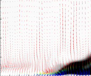
Figure 3 captures the essence of hybrid transition. Velocity perturbation vectors ( $u', v'$ components) are plotted and coloured with the DES shielding function
  $f_d$. The grey-scale contour is the normalized modelled Reynolds stress (
 $-R_{xy}/U_\infty ^2$). It is clear that the perturbations, in the laminar region, are low-frequency ‘jet’-like structures. Although there is a very thin
  $f_d=0$ layer near the wall, as long as it stays within the viscous layer, where the modelled viscosity and Reynolds stresses are nearly zero, the laminar boundary layer is maintained. Then after the breakup of long streamwise streaks, smaller-scale structures are observed, around
  $Re_{x}=1.6\times 10^{5}$. That leads to increase of the shielded region thickness (blue vectors), and increase of modelled Reynolds stress (dark contours). The modelled Reynolds stress adds a RANS component to the representation of turbulence. Small-scale features are damped by the increased subgrid viscosity, but the near-wall perturbations gradually return to a streaky form – a typical behaviour of hybrid simulation.

Figure 3. Velocity perturbation vector (x, y components) coloured by  $f_d$, superimposed on Reynolds shear stress (
 $-R_{xy}/U_\infty ^2$) contour. All quantities are instantaneous.
The evolution of simulation quantities, at the height  $Re_y = 720$ in figure 3, is plotted in figure 4. Figure 4(a) confirms the existence of long large-scale streaks, which lead to small-scale motions after breakup. The appearance of small structures is accompanied by the amplification of fluctuation magnitude. A very distinctive feature in the current simulation is the quick dissipation of small structures where
  $C_{DES}$ rises.

Figure 4. Instantaneous fields along sample line at  $Re_y=720$ on figure 3.
The evolution of the off-diagonal components of test filter quantities  $L_{ij}$ and
  $M_{ij}$ is given in figures 4(c,d). The initial near-zero value, and the later spiking of
  $L_{ij}$, confirm the emergence of small-scale structures. Figures 4(e–h) then explain the fast decrease of
  $L_{ij}$ after transition, i.e. why small scales are dissipated. The modelled kinetic energy and viscosity rise by approximately three orders of magnitude from the laminar to the fully turbulent level. During the climb of the modelled kinetic energy, the shielding function
  $f_d$ decreases from 1 to 0, and the magnitude of the modelled Reynolds shear stress exceeds the resolved part. Note that
  $C_{lim}$ is zero in the laminar region, and then rises to force the length
  $\ell _{LES}$ to exceed
  $\ell _{RANS}$. The DDES formulation switches to the RANS branch if
  $\ell _{LES} > \ell _{RANS}$.
The rise of  $C_{lim}$ is signalled by the grid resolution gauge (2.10), which compares the grid spacing with the estimated
  $\eta$, as shown in figure 4(f). Hence, the switch from nearly wall-resolved LES to hybrid simulation of the turbulent boundary layer (i.e. the modelled transition) is triggered at the location of the physical transition process.
4. Grid sensitivity
Up to this point, the fundamental processes of hybrid transition have been described. Quantitatively, they depend on the grid resolution; as in the case of LES, the model is explicitly a function of the grid. The T3A simulation will be used to demonstrate the grid sensitivity and predictive accuracy. The computational domain and mesh stretching are shown in figure 5. The flat plate starts at  $x=0$ m and is
  $1.5$ m long. The outflow plane is at
  $x=1.5$ m. The inflow plane is at
  $x=-0.05$ m. A zero-gradient condition is placed at the top,
  $y=0.8$ m. The spanwise domain width is
  $0.12$ m.

Figure 5. Computational domain and mesh 0-a-i for T3A.
The various grid resolutions are given in table 1. At the least, a DES simulation should use a mesh that has reached grid convergence for RANS. For that reason, the baseline mesh 1-a-i has the same streamwise and wall-normal resolution as the RANS grid of Ge, Arolla & Durbin (Reference Ge, Arolla and Durbin2014). In the streamwise direction, it has 10 cells before the leading edge (LE in the tables), and another 150 on the plate. The number of cells in the spanwise direction is set to 24, corresponding to an averaged cell aspect ratio of 2. The resolutions of the other cases are adjusted from the baseline mesh. Each mesh name consists of an arabic number, a letter and a roman numeral, to represent different streamwise, spanwise and wall-normal resolutions, respectively.
Table 1. Computational grids for the T3A case.

Figure 6 shows the normalized instantaneous streamwise velocity fluctuation ( $u'/U_\infty$) on the
  $Re_y=1800$ plane (
 $y=0.005$ m). From top to bottom are three typical meshes: 1-b-i, 1-d-i and 3-d-i. All three meshes allow elongated streaks to be captured in the laminar region, though small details are limited by grid cutoff. Refining grid resolution leads to significant increase in resolved flow structure, after the perturbations become nonlinear. For meshes 1-b-i and 1-d-i, detailed structures after transition are missing, but blurry, large, bright (high-velocity) zones are readily apparent in the transition region. For mesh 3-d-i, much richer turbulent structures are resolved after transition.

Figure 6. Normalized instantaneous streamwise velocity fluctuation ( $u'/U_\infty$) for the T3A case on
  $Re_y=180$ (
 $y=0.005$ m) plane. From top to bottom are meshes 1-b-i, 1-d-i and 3-d-i.
Although figure 2 has shown instantaneous flow quantities on a fine mesh, it is informative to consider the same quantities on a coarser grid, mesh 1-b-i, but one that still captures transition. Figure 7 shows the same quantities as figure 2, at  $Re_y=720$, and at the same physical time. The initial phase angles and random vectors of Fourier modes (2.15) are the same as for mesh 3-d-i, so that direct comparison can be made. Figures 7(a) to 7(g) are like low-resolution versions of those in figure 2, but the detailed transition physics is not clearly resolved. Although resolved turbulent spots are missing, bright elongated spots are seen in plots of instantaneous wall-normal velocity, at the location where they would occur. The bright spots, circled in figure 7(a), are close to the location where turbulent spots are seen at finer mesh resolution.

Figure 7. Contours of instantaneous flow quantities at  $Re_y=720$ for mesh 1-b-i.
Without the turbulent spots,  $L_{ij}M_{ij}$ and
  $M_{ij}M_{ij}$ do not change much until the RANS branch is activated to damp them out. Figures 7(e) to 7(g) clearly suggest that the transition prediction mechanism is still tightly associated with the limiting process of (2.9).
Although the flow structure that activates the shielded DES model is poorly resolved on coarse meshes (e.g. 1-b-i), it can be concluded that hybrid simulation makes a plausible prediction of transition, as long as the mesh is not capable of supporting wall-resolved simulation in the fully turbulent region. Essentially, transition is captured because a RANS region becomes established near the wall.
Another perspective on the evolution from resolved Klebanoff modes to turbulent flow is provided by the split between resolved and modelled kinetic energy. Figure 8 plots the mean streamwise evolution of  $\frac 12(u'^2+v'^2+w'^2)$ and modelled turbulent kinetic energy,
  $k$, at
  $Re_y=720$. In the streaky, laminar region, the kinetic energy of resolved fluctuations increases almost linearly with
  $x$ Reynolds number. The modelled kinetic energy remains zero until the transition occurs. Once transition begins, the resolved fluctuation starts to decrease, being partially replaced by modelled kinetic energy. The peak modelled kinetic energy occurs where skin friction also reaches a maximum. In the fully turbulent region, the resolved fluctuations do not become zero, even this near to the wall, which confirms that the adaptive DES model operates as a wall-modelled eddy-resolving simulation.

Figure 8. Streamwise evolution of resolved and modelled turbulent kinetic energy at  $Re_y=720$ for meshes 1-b-i and 3-d-i, averaged in time and spanwise direction.
The time-averaged skin friction coefficient,  $C_f$, along the plate is plotted in figure 9(a). A laminar flow region is missing on mesh 0-a-i: this illustrates that insufficient mesh resolution – streamwise in this case – fails to capture a laminar region and the transition process. (This is also the behaviour that one finds with a fixed value for
  $C_{DES}$, although for a different reason.) It will be shown subsequently, and in § 6.3, that poor resolution locally, near the leading edge, creates a spurious patch of elevated
  $k$. This anomaly, rather than the overall number of grid points, preempts the laminar boundary layer on mesh 0-a-i. Mesh 0-a-i also confirms that the adaptive DES model eventually predicts a RANS boundary layer solution under mesh coarsening.

Figure 9. T3A results. (a) Time-averaged skin friction coefficient along the bottom wall. (b) Instantaneous skin friction coefficient along the bottom wall. (c) Instantaneous spanwise velocity component at  $Re_y\approx 10$. (d) Mesh resolution in plus units; red is streamwise and black spanwise.
On the other meshes, the adaptive DES model is able to correctly predict the skin friction in both laminar and fully turbulent regions. Slight differences exist in turbulent skin friction between meshes, which is related to the RANS–LES coupling along the wall-normal direction.
Meshes 1-a-i to 1-d-i have differing spanwise resolution. With spanwise refinement and increase of cell aspect ratio, the transition location moves upstream, away from the data. Because increasing grid resolution usually improves prediction accuracy, cell aspect ratio may be responsible for this contrary behaviour. To confirm this, streamwise resolution is gradually refined from mesh 1-d-i to meshes 2-d-i and 3-d-i. The mean cell aspect ratios between meshes 1-a-i and 3-d-i are the same, as are meshes 1-b-i and 2-d-i. Mean skin friction predictions on those pairs show that refining the mesh, while keeping the cell aspect ratio fixed, improves agreement with experimental data. An optimal mean aspect ratio is approximately 2, and increasing it may cause an early predicted transition location.
Instantaneous skin friction coefficient ( $C_f$) distributions along the bottom wall, at the same time step, are shown in figure 9(b). Mesh 0-a-i starts in RANS mode immediately at the leading edge, and the fluctuations damp out very quickly. The mesh 1 family shows strong oscillations near the transition location and then the oscillations damp out quickly. Thus, the Reynolds-averaged solution quickly replaces the eddy-resolving simulation after transition, on these meshes. With better streamwise resolution, the oscillation amplitude in the turbulent region becomes stronger (e.g. mesh 3-d-i), which reflects the fact that, after transition, the thickness of the RANS region next to the wall depends on the mesh. This is consistent with an earlier observation that the adaptive DES model approaches the wall-resolved eddy simulation, if mesh resolution is adequate (Yin & Durbin Reference Yin and Durbin2016).
Normalized instantaneous spanwise velocity fluctuation ( $w'/U_\infty$) at the same instant is shown in figure 9(c). The initial low-frequency disturbances in the laminar region are very similar across different mesh resolutions – except for mesh 0-a-i. Mesh 0-a-i shows the earliest deviation from the others, while the rest start to differ only where the
  $C_f$ curves are about to rise. This implies that correct capture of initial disturbances is crucial for predicting a reasonable transition location. The spanwise oscillation amplitude for mesh 3-d-i is considerably larger than the others, which is the same as the observation for skin friction oscillations.
A more general meshing guideline for transition simulation can be concluded from figure 9(d). The local streamwise and spanwise grid resolution in plus units are computed using time-averaged skin friction. The mesh stretching ratios in the streamwise direction are the same, so the only differences are the number of cells and the resulting cell spacing. Looking at the low- $Re_{x}$ range, one sees that the maximum cell spacing to maintain wall-resolved eddy simulation, which is critical in predicting a laminar flow state, is approximately 100 plus units in the streamwise direction, which is violated by 0-a-i. A coarsest spanwise grid spacing is approximately 50 plus units to roughly distinguish the low-frequency disturbances. Figure 9(d) demonstrates that, in the turbulent region, DES allows a much coarser resolution than that in wall-resolved LES, yet maintains a correct turbulent skin friction level. For a practical simulation, it is recommended to limit the streamwise and spanwise grid spacings in regions suspected to be laminar, and perform a mesh convergence study to ensure the correct capture of transition location. Then the mesh can be stretched once the flow becomes turbulent, to achieve an optimal balance between accuracy and efficiency.
5. Test cases
The T3A simulation was used to explain the adaptive DES transition prediction mechanism, and its predictive accuracy in terms of mesh resolution. The simulations in this section illustrate a variety of hybrid simulations of transition. The guiding principle is that the grid and time step should be adequate to resolve the dominant structure of perturbations in the laminar region. The grids have approximately two orders of magnitude fewer points than is needed to fully capture transition, and the subsequent turbulent boundary layer.
Simulations of flat-plate transition corresponding to the rest of the T3 cases are performed, as is the separated flow case of Lardeau et al. (Reference Lardeau, Leschziner and Zaki2012). The inflow parameters for the T3 series are listed in table 2. Most of the  $\omega$ values are adopted from reported RANS simulations (Langtry & Menter Reference Langtry and Menter2005; Ge et al. Reference Ge, Arolla and Durbin2014), for the purpose of bridging the gap between a RANS transition simulation and the current method. The free-stream turbulence decay rate may differ from RANS. As long as the initial low-frequency disturbances are correctly captured, the influence of the
  $\omega$ value on transition location is relatively minor, as will be discussed in § 6.1.
Table 2. Summary of inlet conditions for the T3 flat-plate cases.

5.1. T3B
T3B has approximately twice the inlet turbulent intensity of T3A, as summarized in table 2. The streamwise and wall-normal computational domain size for the T3B simulation is the same as for T3A. Keeping the spanwise cell number fixed required the spanwise length to be reduced nearly by half (0.068 m), in order to capture the Klebanoff streaks. Grid stretching in the wall-normal direction is also adjusted to make sure that  $y^+$ is below 0.8 based on the time-averaged field in the turbulent region. Three meshes at various streamwise resolutions and the same mesh stretching ratio are tested, as listed in table 3.
Table 3. Computational grids for the T3B case.

The time-averaged skin friction coefficient along the streamwise direction is shown in figure 10(a). Mesh 1 is clearly under-resolved, so a near-wall RANS region is active near the leading edge, and physical transition is not captured. Improved streamwise resolution, either mesh 2 or 3, allows a laminar region to occur. Mesh 3 has reached grid convergence; the predicted transition location is slightly delayed and the peak in skin friction is also underestimated, when compared to experiment. Figure 10(b) shows the instantaneous skin friction distribution, which, again, indicates that the amplitude of the resolved fluctuation increases with grid resolution.

Figure 10. T3B results. (a) Time-averaged and (b) instantaneous skin friction coefficient ( $C_f$) along the bottom wall.
5.2. T3A-
T3A- has much lower turbulent intensity (0.874 %) than T3A and T3B, and thus transition is delayed to higher Reynolds number. The computational domain size is  $L_x \times L_y \times L_z = 2.05\ \textrm {m} \times 0.8\ \textrm {m} \times 0.05\ \textrm {m}$. The spanwise length is reduced compared to T3A, so that the spanwise mesh resolution in plus units is at a similar level. The inflow plane is placed at 0.05 m before the leading edge. Table 4 lists the number of grid points in each direction of the tested meshes.
Table 4. Computational grids for the T3A- case.

Again, the mean and instantaneous skin friction coefficient distributions are given in figure 11. The transition location shows a strong dependence on physical time. This causes the instantaneous skin friction to have a much steeper rise at the transition location than the mean curve. Because the inflow turbulent intensity is low for T3A-, the laminar region is very long, which significantly increases the total number of grid points needed to capture the transition location correctly.

Figure 11. T3A- results. (a) Time-averaged and (b) instantaneous skin friction coefficient ( $C_f$) along the bottom wall.
5.3. T3C
The T3C series are flat-plate boundary layers under a pressure gradient. The pressure gradient is created by the contour of the upper boundary and the Reynolds number (table 2). An explicit formula for the upper boundary is given by Suluksna, Dechaumphai & Juntasaro (Reference Suluksna, Dechaumphai and Juntasaro2009). The computational domains of T3C1, T3C2, T3C3 and T3C5 are the same, while T3C4 has an extended region, due to flow separation near the outflow. The spanwise length of the computational domain is 0.1 m. Figure 12 shows the computational domain and the grid point distribution for the T3C1 simulation. Grid stretching in the streamwise direction is adjusted for each case, especially near the leading edge, to avoid spurious activation of shielded RANS at the leading edge. Three mesh resolutions were simulated; table 5 lists the number of grid points in each direction for those meshes.

Figure 12. Computational domain and mesh 1 for T3C1; every other grid point is shown.
Table 5. Computational grids for T3C cases.

Figure 13 shows the mean skin friction coefficient along the bottom wall for all of the T3C family. For T3C1, where transition happens under a favourable pressure gradient, mesh 1 fails to support a laminar region. After refinement of the spanwise resolution, meshes 2 and 3 return correct transition locations and laminar skin friction. However, the turbulent skin friction after transition is underestimated. This underprediction was not observed in the zero-pressure-gradient cases. It is possible that pressure gradient has some negative influence on the grey-area RANS–LES coupling (Spalart et al. Reference Spalart, Deck, Shur, Squires, Strelets and Travin2006) in the wall-normal direction.

Figure 13. Time-averaged surface skin friction coefficient for T3C series. Circles represent experimental data.
The adaptive DES model predicts earlier transition for T3C2 than the experiment, on meshes 1 and 2. The peak of skin friction is therefore predicted too early. Although increased grid resolution in the streamwise direction did not fully capture the peak height of the skin friction curve, the transition location becomes correct.
An excellent match to the transition location and laminar skin friction is achieved for T3C3 on meshes 1 and 2, which is probably due to the grid resolution being better at this lower Reynolds number. Since the transition location is very close to the outflow plane, the skin friction drop right after transition may be a numerical anomaly.
T3C4 imposes difficulty to the turbulence model, as, in the experiment, transition is caused by separation. Since the laminar separation happens close to the outflow, the streamwise length of the computational domain is extended. Most of the plate is covered by laminar flow, which makes grid convergence easily achieved. Since the Reynolds number is lower than in other T3 cases, the same physical grid spacing makes it easier for the turbulence model to capture the right transition location. Although transition location is accurately captured, the skin friction is a bit higher than experiment.
T3C5 is the most challenging among the T3 family, due to it having the highest Reynolds number. Mesh 1 fails to predict the existence of a laminar boundary layer. Increasing spanwise resolution allows the prediction of a laminar region, but the transition location is not correctly predicted. Further increasing streamwise resolution helps in improving the transition length, but not much in the transition location.
Overall, with proper mesh resolution, the adaptive DES model is capable of predicting a laminar boundary layer and the transition location under the effect of pressure gradient. Insight into the grey-area coupling under an adverse pressure gradient may be required to explain the underestimated skin friction in the turbulent regions.
5.4. Flat plate with separation
Transition on a flat plate with separation was first studied by experiment (Lou & Hourmouziadis Reference Lou and Hourmouziadis2000), then by DNS (Wissink & Rodi Reference Wissink and Rodi2006) and LES (Lardeau et al. Reference Lardeau, Leschziner and Zaki2012). It is an idealized configuration of separation-induced transition under an adverse pressure gradient on turbomachinery blades. The LES study of Lardeau et al. (Reference Lardeau, Leschziner and Zaki2012) emphasized the influence of the subgrid model, and the free-stream turbulence intensity and spectrum, on the predicted transition location. It is a challenging case even for LES: the effect of subgrid modelling on separation bubble size is noticeable, even with fine LES resolution. In Yin & Durbin (Reference Yin and Durbin2016), two turbulent intensities (0 % and 1 %) were simulated for this geometry using a mesh resolution equivalent to LES (Lardeau et al. Reference Lardeau, Leschziner and Zaki2012). Good agreement with the dynamic Smagorinsky model was achieved. In order to assess grid sensitivity and requirements for adequate grid resolution, additional grid resolutions and turbulent intensities were tested in the current work. Comparisons are made to DNS (Wissink & Rodi Reference Wissink and Rodi2006) and dynamic Smagorinsky LES data (Lardeau et al. Reference Lardeau, Leschziner and Zaki2012).
The mesh is described in table 6. The geometry and mesh clustering are shown in figure 14. The inflow plane is placed at  $0.5L$ before the plate leading edge, where
  $L$ represents the chord length. The plate leading edge is placed at
  $x/L=0$. The outflow is at
  $1.5L$ downstream of the leading edge. The adverse pressure gradient that causes flow separation is created by the divergence of the upper slip wall.
Table 6. Computational grids for the flat-plate separation case. Meshes 1, 2, 3 and 4 share the same stretching ratio. Meshes 1-a and 2-a have more clustering placed near the leading edge.


Figure 14. Mesh 1 for the separated flat-plate case, showing every other grid line for the coarsest mesh.
Inflow conditions were created by the method mentioned in § 2.2. The parameter  $\kappa _e$ in (2.11) was fixed at
  $0.015/L$. Reference data are available from LES (Lardeau et al. Reference Lardeau, Leschziner and Zaki2012) for
  $Tu = 0$ % to 2 % and from DNS (Wissink & Rodi Reference Wissink and Rodi2006) for
  $Tu = 1$ %.
Good agreement with LES data is achieved at different turbulent intensities on mesh 4, as shown in figure 15(a). Since the adaptive DES model behaves like the dynamic Smagorinsky model in fully eddy simulation regions, it is expected that the evolution of turbulent intensity would match well with LES data. Figure 15(b) shows the streamwise turbulent intensity on various meshes; slight sensitivity to the grid resolution is observed. Note that the streamwise decay of turbulent intensity predicted in LES does not match with DNS (Lardeau et al. Reference Lardeau, Leschziner and Zaki2012). The current simulation, is targeted to matching LES data.

Figure 15. Resolved turbulent intensity profiles along the streamwise direction at  $y/L = 0.065$ on mesh 4: (a) at various targeted inflow turbulent intensities, compared with LES; and (b) at varying mesh resolution for the
  $Tu=1\,\%$ case using consistent boundary condition.
Figure 16 shows the skin friction coefficient along the bottom wall, and the shape of the separation bubble for  $Tu = 0\,\%$. The predicted transition to turbulence is not very sensitive to grid resolution. There is a remarkable resemblance in the shear layer prediction of figure 16(b) between meshes 3 and 4. A similar resemblance is also observed between meshes 1 and 2; this suggests that sensitivity to mesh resolution in the spanwise direction is less than in the streamwise direction. Thus, without inflow fluctuations, the development of the separated shear layer is not very sensitive to spanwise resolution. This is due to the flow structures during the initial development of Kelvin–Helmholtz instability being nearly two-dimensional. Meshes 1 and 2 predict an earlier breakup of the separated shear layer than meshes 3 and 4. Overall, the adaptive DES model predicts a smaller separation bubble than LES. Mesh 1 is the closest to LES data, and refining the resolution increases the deviation.

Figure 16.  $Tu = 0\,\%$ results: (a) skin friction coefficient on the bottom wall; and (b) separation bubble.
Similar plots are made for  $Tu = 1\,\%$ in figure 17. Note that the reference LES data using the dynamic Smagorinsky subgrid model predicts a much earlier reattachment than DNS. The predicted skin friction and separation bubble using adaptive DES on meshes 3 and 4 are in excellent agreement with LES data. Given that mesh 4 has the same number of grid points as the LES simulation, such behaviour suggests that the adaptive DES model converges to wall-resolved eddy simulation on fine meshes. Again, the predicted skin friction and separation bubble length on meshes 1 and 2 agree with DNS better than with LES. The height of the separation bubble is overestimated on meshes 1 and 2.

Figure 17.  $Tu = 1\,\%$ results: (a) skin friction coefficient on the bottom wall; and (b) separation bubble.
Simulations are also performed at  $Tu=2\,\%$, for which only LES data are available. Stronger turbulent intensity appears to increase grid sensitivity for the adaptive DES model. Meshes 1 and 2 fail to predict a laminar boundary layer before separation, as shown in figure 18(a). To show that the leading-edge spacing, where the boundary condition is discontinuous, causes this failure, two more meshes (1-a and 2-a) were created by adjusting the grid stretching of meshes 1 and 2. They have the same streamwise grid spacing at the leading edge as meshes 3 and 4. On those meshes, both the separated shear layer and the upstream boundary layer are laminar. Mesh clustering at the leading edge means coarser streamwise resolution in the separated flow region. Hence, the upstream region is correct, but the reattachment is too far downstream, in figure 18.

Figure 18.  $Tu = 2\,\%$ results: (a) skin friction coefficient on the bottom wall; and (b) separation bubble.
Figure 19 shows the isosurfaces of instantaneous velocity fluctuation on meshes 1-a and 4 with turbulent intensities of 1 % and 2 %. The mesh on the bottom wall is also shown, for reference. Note that the appearance and size of streaks at the upstream edge of the separated shear layer are correctly captured on both meshes. After the breakup of those streaks, mesh 4 is capable of resolving a much richer content of small-scale structures than mesh 1-a. The discrepancy in instantaneous flow structures is more obvious at higher turbulent intensity. The isosurfaces suggest that resolving the small scales, inside the separated shear layer, might be critical for capturing the correct size of the separation bubble. So, the issue here is not so much predicting transition as capturing mixing in the separated layer, which is responsible for reattachment.

Figure 19. Isosurfaces of  $u'=\pm 0.2U_\infty$ on meshes 1-a (lower) and 4 (upper) for (a)
  $Tu = 1\,\%$ and (b)
  $Tu = 2\,\%$.
6. Discussion
6.1. Sensitivity to inflow conditions
The choice of inflow conditions in the previous test cases is one of a few possible combinations. In the current simulation, the inflow velocity and turbulent kinetic energy (TKE) boundary conditions rely on the assumption that the velocity field contains the resolved turbulent fluctuations, and the kinetic energy represents the unresolved part. So the resolved part is synthesized and the unresolved part is represented by  $k$ (as the
  $k$ in
  $k$–
$k$– $\omega$ transport equations). However, the T3A simulation shows that the correct capture of initial low-frequency disturbances inside the laminar boundary layer may determine the transition location – the ability of low frequencies to penetrate the boundary layer has been explained by theory (Zaki & Durbin Reference Zaki and Durbin2005). Thus, modelling the high-frequency motions in the free stream may not be critical. Although the meshes have coarser resolution than DNS, they are still capable of correctly resolving the low-frequency motions. So another option is to put all the energy in the resolved inflow spectrum, and let the modelled kinetic energy be zero. To compare the two options, a T3A simulation using an inflow with a full velocity spectrum, and zero modelled
  $k$, is performed on mesh 1-b-i. It is shown by the green dash-dotted line in figure 20(a). The difference from the original method is minimal. Thus, modelling the high-frequency motions at the inflow is unnecessary for this case; the present inflow velocity and
  $k$ condition are only aimed at a better physical representation. The blue and red curves in figure 20(a) show the sensitivity of transition location to the total
  $k$ at inflow, which is consistent with higher free-stream TKE leading to earlier transition.

Figure 20. Sensitivity with inflow condition of skin friction: (a) total (resolved  $+$ modelled) TKE; and (b) eddy frequency.
The current simulations use an  $\omega$ value estimated from the energy spectrum (integral scale). Another way of setting
  $\omega$ at inflow is to estimate it from its transport equation: the equilibrium solution of (2.2) is
 \begin{equation} \omega^2 = \frac{2 C_{\omega 1}}{C_{\omega 2}} |S|^2. \end{equation}
T3A simulations on mesh 1-b-i are performed to examine the sensitivity to the  $\omega$ inflow value. The predicted skin friction curves are shown in figure 20(b). Switching to the equilibrium value (black line) results in a very similar skin friction curve to the original value (red dashed and double dotted line). Increasing
  $\omega$ postpones transition, which is also reported in RANS simulations (Ge et al. Reference Ge, Arolla and Durbin2014). However, reducing its value has almost no effect on the transition location. Overall, the sensitivity of transition location to
  $\omega$ is not as strong as that observed in RANS simulations (Ge et al. Reference Ge, Arolla and Durbin2014).
6.2. The role of  $C_{dyn}$ and $C_{lim}$


Earlier, in § 3, the dominant role of  $C_{lim}$ (2.9) in predicting transition was noted. However, the role of
  $C_{dyn}$ in the same equation is still unclear. To explore the effect of
  $C_{dyn}$, the T3A simulation on mesh 3-d-i was re-run, with (2.9) replaced by
 \begin{equation} C_{DES} = \max( 0, C_{lim} ) = C_{lim} . \end{equation}
This is equivalent to setting  $C_{dyn}=0$. The statistical average is again performed in both time (
 $0.4$ s, unchanged) and span (48 layers). A comparison is made in figure 21. The skin friction in the turbulent region is more oscillatory when (6.2) is used. In well-resolved simulations,
  $C_{dyn}>C_{lim}$. When that is true in the fully turbulent region, (6.2) reduces the subgrid viscosity. The earlier transition when
  $C_{dyn}=0$ shows that there are places in the transition zone where
  $C_{dyn}$ is determining
  $C_{DES}$ and is damping fluctuations. Nevertheless,
  $C_{lim}$ plays a major role in how the model captures transition.

Figure 21. Skin friction predicted on mesh 3-d-i of T3A, with dynamic procedure or just forced  $C_{lim}$.
6.3. Leading-edge grid spacing
The T3A simulations on the coarsest mesh, 0-a-i, failed to capture a laminar boundary layer at the leading edge; the same behaviour was observed on mesh 1 in § 5.4, where it was resolved by refining the leading-edge resolution (mesh 1-a).
An explanation of the spurious behaviour on coarse grids is provided by figure 22. This compares contours of time-averaged modelled TKE ( $k/U_\infty ^2$) near the leading edge for meshes 0-a-i and 1-b-i: note that figure 22 is a zoomed view; the whole domain is
  $-0.05<x<1.5$. Numerical tests were performed with initial conditions of stationary flow, uniform free-stream laminar flow and a converged fully turbulent RANS solution. This spurious behaviour of the modelled turbulent kinetic energy persists on the coarsest mesh, regardless of initial condition.

Figure 22. Normalized modelled TKE ( $k/U_\infty ^2$) at the leading edge on meshes 0-a-i and 1-b-i for T3A.
The two cases have low modelled  $k$ in the free stream. However, near the leading edge, their behaviours are quite different. On mesh 0-a-i, where leading-edge spacing is larger, and there are fewer points upstream of the leading edge, spurious TKE is found to accumulate just upstream of the leading edge. This appears to be an anomaly of the underlying
  $k$–
$k$– $\omega$ model, similar to the well-known stagnation point anomaly. This spurious modelled
  $k$ then enters into the boundary layer. The boundary layer is immediately turbulent and the RANS branch is activated. By contrast, the modelled TKE on mesh 1-b-i is low in the vicinity of the leading edge. The newly formed boundary layer has near-zero TKE and is laminar.
As a general rule for simulating transitional flow, the leading-edge grid must be fine enough to avoid spurious  $k$, so that a laminar boundary layer can be captured. The cause of failure is readily apparent and can be fixed.
7. Conclusion
The current research explores the capability of the adaptive  $\ell ^2$–
 $\omega$ DES model to predict laminar-to-turbulent transition with free-stream turbulence and pressure gradients. Test cases include bypass transition at zero and varying pressure gradients, and separation-induced transition. Comparisons with data show that the adaptive model is capable of predicting transition without the help of intermittency functions or data correlations. Adaptivity based on resolved physics plays an important role: low-frequency precursors in the incident laminar boundary layer are captured because the model computes a value of
  $C_{DES}$ that is nearly zero when the perturbations are well resolved. The transition location is captured by simulation of the initial breakdown of these perturbations. It need not be highly resolved.
Transition is emulated, as the model computes a higher value of  $C_{DES}$. This is caused by velocity gradients that produce
  $k$. Then, assuming the mesh cannot resolve near-wall turbulence, a shielded RANS wall layer is activated during the transition process. This causes the skin friction to increase. The adaptive DES model automatically balances the resolved and unresolved portions in the turbulent region.
For laminar separation followed by transition in the shear layer, the adaptive DES acts as a subgrid model, to capture the separated shear layer. Flow structures inside the laminar shear layer and their breakup are physically resolved, if the mesh supports it. At the same time, mesh sensitivity studies show that the separation bubble size is sensitive to mesh resolution in both the streamwise and spanwise directions, which is related to capturing mixing in the separated shear layer, rather than transition.
Acknowledgements
The numerical computations were performed using  ${\rm \pi}$ 2.0 at the Center for High Performance Computing, Shanghai Jiao Tong University.
Funding
The authors gratefully acknowledge financial support from the National Natural Science Foundation of China (no. 12002210).
Declaration of interests
The authors report no conflict of interest.


