
Introduction
Despite judicial independence being one of the principles embraced in most democratic constitutions, recent studies of judicial politics have made it clear that it is inadequately established in most of these countries. Although the concept has several aspects, ‘[i]ndependence of the judiciary means: (1) that every judge is free to decide matters … without any improper influences … (2) that the judiciary is independent of the executive and legislature’.Footnote 1 This definition seems to reflect consensus among scholars.Footnote 2 Putting aside the strategic behavior of the court vis-à-vis other branches of the government (Epstein and Knight, Reference Epstein and Knight1998), the principal-agent theory tells us that one of threats to judicial independence is appointment power. When the president, the prime minster, or legislators can hire and fire judges, the latter end up making decisions to please the former (Ramseyer and Rasmusen, Reference Ramseyer and Rasmusen2003; Ramseyer and Rosenbluth, Reference Ramseyer and Rosenbluth1993: chs. 8–9, Reference Ramseyer and Rosenbluth1998: ch. 6). Similarly, reappointment and promotion also matter. The ‘Universal Declaration on the Independence of Justice’ warns that ‘[t]he assignment of a judge to a post within the court to which he is appointed is an internal administrative function to be carried out by the judiciary’. Otherwise, ‘there is a danger of erosion of judicial independence by outside interference. It is vital that the court not make assignment as a result of any bias or prejudice or in response to external pressure’ (Shetreet and Deschênes, Reference Shetreet and Deschênes1985: 451). The typical test of judicial independence is whether judges of the same opinion as the executive are promoted more often than others (Maitra and Smyth, Reference Maitra and Smyth2004; Salzberger and Fenn, Reference Salzberger and Fenn1999).
The Japanese judicature is a good case with which to run this test because it is one of the allegedly-most dependent judiciary branches. On the one hand, Article 76 of the Japanese Constitution stipulates that all judges shall be independent in the exercise of their conscience and shall be bound only by the Constitution and the laws. On the other hand, Article 79 provides the Cabinet with the power to designate a Chief Supreme Court Judge (appointed by the Emperor) and to appoint other Supreme Court Judges. According to Article 80, the judges of the inferior courts shall be nominated by the Supreme Court and appointed by the Cabinet. Ramseyer and Rasmusen (Reference Ramseyer and Rasmusen2003) argue that the existence of Articles 79 and 80 (stipulating Cabinet control of judicial promotion) means that in practice, even though judicial independence is guaranteed by Article 76, Japanese judges routinely validate what the government has done.Footnote 3 Thus, judicial independence is questioned. They provide evidence for this claim by conducting a series of statistical tests, which indicate that judges with leftist preferences do worse in their careers. Their argument has been very influential and is frequently cited, not only in Japanese studies but also in the comparative (judicial) politics literature, which refers to the Japanese judicature as one of the least independent judiciaries (e.g. Ginsburg, Reference Ginsburg2003: 24; Hall, Reference Hall, Hall and McGuire2005: 76–7; Solomon, Reference Solomon2007: 127).
We suggest that their dataset is incorrect to hold up their argument, the statistical methods they use are in fact inadequate to assess whether or not Japanese judges are dependent, and their research design is not appropriate for their own research agenda in the first place.
Among their findings, we focus on their first evidence (Ramseyer and Rasmusen, Reference Ramseyer and Rasmusen2003: Table 2.6), that is, the analysis to suggest that a judge who once belonged to a leftist group will take longer to reach the position of ‘division chief’ (sokatsu in Japanese; a ‘moderately prestigious status’) during the period of conservative dominance of post-war Japan.Footnote 4 Their findings consist of an OLS model that regresses the time taken for a judge to become division chief on a dummy variable identifying whether the judge once belonged to a leftist group. On closer analysis, however, some of the judges in the dataset used had not yet reached the position of division chief and therefore have no value on the dependent variable. This problem is called censoring. Some retire or die without reaching this position; some are too young to reach this position, and others skip this position by taking an irregular career path. Ramseyer and Rasmusen (Reference Ramseyer and Rasmusen2003) either drop those judges from their data set, or keep them in the dataset with arbitrary values substituted. We suspect that this procedure of data manipulation causes bias in their estimates.
In this article, we use the statistical technique of survival analysis. This enables researchers to examine how independent variables affect dependent variables that may or may not be censored. To address the problem that some judges may never become division chiefs, we employ a split population model of survival analysis. We also attempt to deal with the issue of what happens when a judge takes an irregular career path by using left truncation. To our knowledge, for the first time, we propose a survival analysis model that deals simultaneously with the problems of split population and left truncation.
We also extend the causal inference literature to censored, time-to-event data. We match every leftist judge with her non-leftist counterpart so that most variables are controlled and omitted variable bias is unlikely. We estimate the average treatment effects on two dependent variables, Time and Event. In particular, in the case of Time, after matching, we drop not only judges whose time is censored but also their corresponding judges so that most variables continue to be controlled.
Our findings indicate that leftist judges are by no means discriminated in terms of the timing and occurrence of promotion, against the argument of Ramseyer and Rasmusen (Reference Ramseyer and Rasmusen2003). Note that this result can be interpreted as either judicial independence or dependence; both are observationally equivalent. We are simply unable to tell whether leftist judges behave as they do because they want to, or because they fear the punishment from the conservative government. Though Ramseyer and Rasmusen (Reference Ramseyer and Rasmusen2003) present other evidence that leftist judges or judges who issue rulings against the government are discriminated against in terms of promotion, this very fact is, against their argument, good evidence that the judiciary is independent of the executive. Judicial independence necessitates that the government acts to promote its followers and punishes those who protest its policies. On the contrary, in systems where government control of the judiciary is stronger, judges may not express any conflict with the executive branch. Therefore, the executive need not discriminate any judges for political reasons.
This article proceeds as follows. In the next section, the argument made by Ramseyer and Rasmusen (Reference Ramseyer and Rasmusen2003) is briefly reviewed and one of their regression analyses is replicated. The following section reconsiders how to analyze their data. To begin, survival analysis, left truncation, and split population models are explained. Then, we discuss the issue of causal inference and propose a new way to estimate average treatment effects on time and event. The subsequent section reanalyzes their data. First, their data are corrected. Second, we perform the matching procedure, check the balance of covariates and their interactions, and estimate average treatment effects on time and event. Third, we apply survival analysis to the matched data. The final section concludes with a summary of the findings and a brief discussion of judicial independence in general as well as other possible applications of our method.
Replication
Ramseyer and Rasmusen (Reference Ramseyer and Rasmusen2003) argue that judges with leftist preferences do worse in their careers. They suggest that Japanese courts use job postings as incentives and judges uphold the conservative positions of the longtime incumbent Liberal Democratic Party. Among various statistical analyses, Ramseyer and Rasmusen (Reference Ramseyer and Rasmusen2003) use the career data of 501 judges, and show that judges who once joined a leftist group were promoted more slowly than their peers. In this article, we begin by replicating the statistical analysis of judicial careers reported in Ramseyer and Rasmusen (Reference Ramseyer and Rasmusen2003: 41).
Ramseyer and Rasmusen (Reference Ramseyer and Rasmusen2003: 39) compiled judicial career data for all Japanese judges hired between 1959 and 1968 using a list that details all the posts held by these judges (Nihon Minshu Horitsuka Kyokai Shiho Seido Iinkai, 1998). Although it would be ideal to have salary information for these judges, there are no such data available. Instead, they focus on the time it takes for a judge to reach the status of division chief. This is somewhat justified as a substitution because it is not until judges become the chief judge that salaries among their cohort begin to differ. The dependent variable, Time_Chief, is defined as the year a judge first received a division chief appointment, less the year she graduated from the Legal Research and Training Institute.Footnote 5
Ramseyer and Rasmusen (Reference Ramseyer and Rasmusen2003) make two main adjustments. First, they drop those judges who held non-judicial postings (generally regarded as prestigious) in the two years before their first division chief posting (Ramseyer and Rasmusen Reference Ramseyer and Rasmusen2003 call them ‘stars’). In the rare cases where a judge served as court chief judge before serving as division chief judge, they treat this former position as the division chief posting, since such an appointment is unambiguously higher than division chief. Second, they drop the group of 164 judges who (i) never obtained a division chief appointment and (ii) quit or died before the mean Time_Chief for the rest of the group, which is 20.41 years (we call this group ‘dropouts’). This is because these judges have no value of Time_Chief. They kept, however, the 83 judges who quit or died after 20.41 years without an appointment to division chief and treated their death or resignation as their time of first division chief appointment (we call this group ‘losers’). Also, they treat the judges who did not have a division chief appointment as of 1997 (the last year the list of judges reports career data) as becoming a division chief in 1997. In addition to these adjustments, Ramseyer and Rasmusen (Reference Ramseyer and Rasmusen2003) drop judges who did not join the court within a year of graduating from the Legal Research and Training Institute (mostly, those who first became a prosecutor or attorney and later joined the court). Of 797 judges listed for the period between 1959 and 1968, 501 remain in the career data set.
To test for political discrimination, Ramseyer and Rasmusen (Reference Ramseyer and Rasmusen2003) introduce a key independent variable named Leftist, which takes the value 1 if a judge was a member of the communist-leaning Young Jurists League (YJL) in 1969 and 0 otherwise.Footnote 6 They hypothesize that leftist judges are discriminated against in salary, and expect that, in a regression model of Time_Chief, the coefficient for Leftist would be statistically significant and positive.
Judges may be promoted not because they are favored for political reasons, but because they are talented. In order to control for quality of judge, the authors use three control variables. Flunks is defined as the number of times a judge failed the entrance exam to the Legal Research and Training Institute, which is estimated from passage year and birth year.Footnote 7Elite_College takes the value 1 if a judge graduated from either the University of Tokyo or the University of Kyoto, two of the most prestigious national universities in Japan, and 0 otherwise.Footnote 81st_Tokyo takes the value 1 if a judge started at the Tokyo District Court and 0 otherwise, accounting for the fact that the most promising are generally assigned to the Tokyo District Court.Footnote 9
In order to control for unobservable differences among the cohorts, dummy variables indicating the year in which a judge finished her legal education are incorporated into estimation.Footnote 10
We replicate the OLS results in Ramseyer and Rasmusen (Reference Ramseyer and Rasmusen2003: 41) and display it in the left half of Table 1.Footnote 11 From their perspective, what is most notable is the coefficient of 0.919 for Leftist, which has a statistical significance of 0.088. This implies that judges who were members of the YJL in 1969 received their first division chief assignment roughly a year later than their non-YJL peers, controlling for these other factors.
Table 1. OLS results of Time to division chief
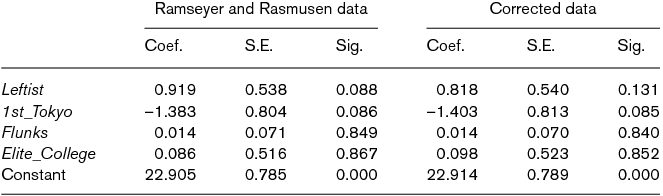
Note: N = 501. The coefficients for cohort dummies are not reported. Significance is based on a two-tailed test. For both models, adjusted R2 is 0.09.
Reconsideration
The way Ramseyer and Rasmusen (Reference Ramseyer and Rasmusen2003) handle and analyze the data, which we replicate above, have some problems, as we mentioned in the Introduction. To address these problems, we employ survival analysis, matching, and average treatment effects, which we elaborate on below.
Survival analysis
Latent time and censoring
We define latent time as the unobservable years a judge would have needed to receive a division chief appointment if the judge remained in the court until that moment. We say latent time is ‘censored’ if it ends without reaching a division chief post. Examples are ‘dropouts’ and ‘losers’ who quit or died early in their careers without obtaining a division chief appointment. If judges have not yet obtained a division chief appointment in 1997, the end year the data covers, their latent time is also censored. For judges whose latent time is censored, Time_Chief is not observed. Ramseyer and Rasmusen (Reference Ramseyer and Rasmusen2003) exclude the ‘dropouts’ from their dataset and assume Time_Chief as the time of censoring for the losers and the judges yet to become division chiefs in 1997. These adjustments, however, are problematic. The censored judges would receive a division chief posting some day in future if they had not died or continued to serve as a judge. Their true Time_Chief is longer than their presumed Time_Chief. Thus, the manipulation by Ramseyer and Rasmusen (Reference Ramseyer and Rasmusen2003) underestimates Time_Chief and causes bias in estimating their key coefficient, the effect of Leftist on Time_Chief.
Survival analysis is a set of statistical techniques designed to address censored latent time. It deals simultaneously with the questions of if an event occurs and when it occurs (e.g., if a judge becomes division chief and how long the judge takes to reach the position).Footnote 12 We introduce a set of new variables. First, Event takes the value 1 if a judge received a division chief posting and 0 otherwise. While Ramseyer and Rasmusen (Reference Ramseyer and Rasmusen2003) dropped the ‘stars’, we keep them in our data set (Event = 1) and take into account the time they held non-judicial postings with the method we will explain later. We also keep the ‘dropouts’ in our data (Event = 0). Second, Time is defined as the years a judge needs to receive a division chief appointment (or to be censored without reaching division chief) after their graduation from the Legal Research and Training Institute. Note that both Time and Time_Chief measure the time a judge takes to reach the first division chief post, although the former is defined as one year greater than the latter. The former is thus amenable to logarithmic transformation.
Let D, T, and T* denote Event, Time, and latent time, respectively. We assume T* follows a log logistic distribution, whose probability density function is
 \begin{equation*}
f(T^{\ast}) = \frac{{\frac{s}{m}\left( {\frac{{T^*}}{m}} \right)^{s - 1} }}{{\left( {1 + \left( {\frac{{T^{\ast}}}{m}} \right)^s } \right)^2 }},
\end{equation*}
\begin{equation*}
f(T^{\ast}) = \frac{{\frac{s}{m}\left( {\frac{{T^*}}{m}} \right)^{s - 1} }}{{\left( {1 + \left( {\frac{{T^{\ast}}}{m}} \right)^s } \right)^2 }},
\end{equation*}
where m is the scale parameter as well as the median of T* and s is the shape parameter. We are interested in what factors increase or decrease m, which is always positive. Thus, the logarithm of m is explained by linear combination of covariates W and coefficients b
 \begin{equation*}
m = \exp (bW).
\end{equation*}
\begin{equation*}
m = \exp (bW).
\end{equation*}
If we observe that a judge becomes division chief (Event = 1), its contribution to likelihood is proportional to
 \begin{equation*}
f(T) = \frac{{\frac{s}{{\exp (bW)}}\left( {\frac{T}{{\exp (bW)}}} \right)^{s - 1} }}{{\left( {1 + \left( {\frac{T}{{\exp (bW)}}} \right)^s } \right)^2 }}.
\end{equation*}
\begin{equation*}
f(T) = \frac{{\frac{s}{{\exp (bW)}}\left( {\frac{T}{{\exp (bW)}}} \right)^{s - 1} }}{{\left( {1 + \left( {\frac{T}{{\exp (bW)}}} \right)^s } \right)^2 }}.
\end{equation*}
If a judge has not become division chief before censoring (Event = 0), its contribution to likelihood is proportional to the probability of survival
 \begin{equation*}
S(T) = \int\limits_T^\infty {f(T^{\ast})} dT^{\ast} = \frac{1}{{1 + \left( {\frac{T}{m}} \right)^s }} = \frac{1}{{1 + \left( {\frac{T}{{\exp (bW)}}} \right)^s }}.
\end{equation*}
\begin{equation*}
S(T) = \int\limits_T^\infty {f(T^{\ast})} dT^{\ast} = \frac{1}{{1 + \left( {\frac{T}{m}} \right)^s }} = \frac{1}{{1 + \left( {\frac{T}{{\exp (bW)}}} \right)^s }}.
\end{equation*}
Parameters are estimated by maximizing total likelihood.
Left truncation
Suppose that a judge held a non-judicial post (i.e., officers in the Secretariat of the Supreme Court or the Ministry of Justice) at the 10th year of her career, came back to the court in the 14th year, and became division chief in the 20th year. In this case, her latent time as a judge is censored at the 10th year (Time = 10, Event = 0), since she had no chance of becoming division chief while holding a non-judicial post. Her second latent time (or observation) resumes at the 14th year and ends with division chief post (Time = 20, event = 1). Note that she has no way of reaching a division chief post for the period up to the 14th year in terms of her second latent time. Thus, we should discount the 20 years she needed to reach a division chief post. This is called ‘left truncation’ in survival analysis. We introduce a new variable, Begin (T 0), which is defined as the years a judge takes to resume a judicial posting since graduation from the Legal Research and Training Institute. In the above example, Begin has a value of 14. Thus, a judge is assumed to have more than one latent time if she resumes a judicial career after censoring.
When latent time restarts at T 0, both survival probability and failure density are conditioned on the fact that an event has not happened by T 0, whose survival probability is S(T 0). Thus, the conditional survival probability and the conditional probability density at T > T 0 are S(T)/S(T 0) and f(T)/S(T 0), respectively.
Split population
Ramseyer and Rasmusen (Reference Ramseyer and Rasmusen2003) implicitly assume that all judges eventually become division chief. This assumption is dubious, however. If leftist judges are severely discriminated, some of them should never be on the promotion track. In split population modeling, the population of observations is divided into two groups, one that would end up with promotion to division chief if it is not censored (on the promotion track) and one that would not even without being censored (off the promotion track). If a judge becomes division chief, we know that the judge is on the promotion track. But, if a judge's career is censored, we are not sure whether the judge is off the promotion track or the judge on the promotion track has not become division chief yet. Thus, we estimate how likely judges are to be on the promotion track, instead of measuring whether they are.
Let r be the probability for a judge i to be on the promotion track. Then, the probability to be censored at T (D = 0) is the probability that a judge is off the track, plus the probability that a judge on the track has not become division chief at T: (1− r) + rS(T). The probability density to become division chief at T is the probability that a judge is on the track, times the probability density that the judge becomes division chief at T: rf(T). Moreover, we explain r by logistic function of linear combination of some covariates Z and coefficients a
 \begin{equation*}
r = \frac{1}{{1 + \exp ( - aZ)}}.
\end{equation*}
\begin{equation*}
r = \frac{1}{{1 + \exp ( - aZ)}}.
\end{equation*}
To sum, likelihood of a judge who becomes division chief at T is proportional to rf(T)/S(T 0), namely
 \begin{equation*}
\frac{1}{{1 + \exp ( - aZ)}}{{\frac{{\frac{s}{{\exp (bW)}}\left( {\frac{T}{{\exp (bW)}}} \right)^{s - 1} }}{{\left( {1 + \left( {\frac{T}{{\exp (bW)}}} \right)^s } \right)^2 }}} \mathord{\left/
{\vphantom {{\frac{{\frac{s}{{\exp (bW)}}\left( {\frac{T}{{\exp (bW)}}} \right)^{s - 1} }}{{\left( {1 + \left( {\frac{T}{{\exp (bW)}}} \right)^s } \right)^2 }}} {\frac{1}{{1 + \left( {\frac{{T0}}{{\exp (bW)}}} \right)^s }}}}} \right.} {\frac{1}{{1 + \left( {\frac{{T0}}{{\exp (bW)}}} \right)^s }}}},
\end{equation*}
\begin{equation*}
\frac{1}{{1 + \exp ( - aZ)}}{{\frac{{\frac{s}{{\exp (bW)}}\left( {\frac{T}{{\exp (bW)}}} \right)^{s - 1} }}{{\left( {1 + \left( {\frac{T}{{\exp (bW)}}} \right)^s } \right)^2 }}} \mathord{\left/
{\vphantom {{\frac{{\frac{s}{{\exp (bW)}}\left( {\frac{T}{{\exp (bW)}}} \right)^{s - 1} }}{{\left( {1 + \left( {\frac{T}{{\exp (bW)}}} \right)^s } \right)^2 }}} {\frac{1}{{1 + \left( {\frac{{T0}}{{\exp (bW)}}} \right)^s }}}}} \right.} {\frac{1}{{1 + \left( {\frac{{T0}}{{\exp (bW)}}} \right)^s }}}},
\end{equation*}
and likelihood of a judge who is censored (ceases to be observed without becoming division chief) at T is proportional to (1–r)+rS(T)/S(T 0), that is
 \begin{equation*}
\frac{1}{{1 + \exp (aZ)}} + \left( {\frac{1}{{1 + \exp ( - aZ)}}{{\frac{1}{{1 + \left( {\frac{T}{{\exp (bW)}}} \right)^s }}} \mathord{\left/
{\vphantom {{\frac{1}{{1 + \left( {\frac{T}{{\exp (bW)}}} \right)^s }}} {\frac{1}{{1 + \left( {\frac{{T0}}{{\exp (bW)}}} \right)^s }}}}} \right.} {\frac{1}{{1 + \left( {\frac{{T0}}{{\exp (bW)}}} \right)^s }}}}} \right).
\end{equation*}
\begin{equation*}
\frac{1}{{1 + \exp (aZ)}} + \left( {\frac{1}{{1 + \exp ( - aZ)}}{{\frac{1}{{1 + \left( {\frac{T}{{\exp (bW)}}} \right)^s }}} \mathord{\left/
{\vphantom {{\frac{1}{{1 + \left( {\frac{T}{{\exp (bW)}}} \right)^s }}} {\frac{1}{{1 + \left( {\frac{{T0}}{{\exp (bW)}}} \right)^s }}}}} \right.} {\frac{1}{{1 + \left( {\frac{{T0}}{{\exp (bW)}}} \right)^s }}}}} \right).
\end{equation*}
Given the data D, T, T 0, W, and Z, the parameters (a,b, and s) are estimated so that the total likelihood is maximized.Footnote 13
Matching and average treatment effects
Even if we try to specify the model, taking into account every factor we need to, we are unlikely to do it perfectly. Latent time T* may not follow a log logistic distribution and the population split function may be probit instead of logistic, though we cannot be sure. We simply cannot avoid model-dependent results in the application of any parametric model to raw data.Footnote 14
The causal inference literature takes model dependence seriously and aims to ameliorate it. One way to do this is matching the data and estimating the average treatment effect, which we explain below. These methods, however, have rarely been applied to censored time-to-event data. Bland and Altman (Reference Bland and Altman1994) lament ‘[s]ometimes there is no suitable method of matched analysis, as in survival analysis’. This is because we cannot observe the values of (unobserved) latent time T* of all units because of censoring. Below, we propose a new way to estimate the average treatment effect for both (unobserved) latent time T* and Event D.
Average treatment effect on event
Following the potential outcome framework, we assume that Event D for judge i, Di, takes the value of D 1i if judge i belongs to the leftist group, YJL, and Di = D 0i otherwise. Hence, the effect of Leftist on Event Di for judge i should be D 1i– D 0i. One of the quantities of interest for most scholars is called the ‘average treatment effect’ in the causal inference literature and is expressed as
 \begin{equation*}
\frac{1}{n}\sum\limits_{i = 1}^n {D_{1i} } - D_{0i} .
\end{equation*}
\begin{equation*}
\frac{1}{n}\sum\limits_{i = 1}^n {D_{1i} } - D_{0i} .
\end{equation*}
Here, ‘the fundamental problem of causal inference’ (Holland, Reference Holland1986) arises because we can only observe D 1i or D 0i, not both. Let X be a dummy variable of Leftist (which is called ‘treatment’ in the literature of causal inference). If Xi = 1, we observe D 1i but not D 0i. If Xi = 0, we observe D 0i but not D 1i. How can we estimate the average treatment effect?
One way is matching. Let M be a vector of all measured covariates. Consider a matching function j = m(i) that satisfies Mi = Mj and Xi = 1–Xj. We match judge m(i) to judge i. For example, YJL Judge Tsutomu Ueno (X = 1) is matched to non-YJL Judge Kohei Araki (X = 0). Both were born in 1933, graduated from non-elite universities (Elite_College = 0), became a judge in 1959 (Flunks = 1959–1933–24 = 2, where 24 is the youngest age for a college graduate to become a judge), started their careers outside of Tokyo (1st_Tokyo = 0), and reached division chief without leaving the court (Begin = 0).
We estimate the average treatment effect on event by the difference in means between Event of YJL judges and that of non-YJL judges
 \begin{eqnarray*}
&& \frac{1}{n}\sum\limits_{i = 1}^n \, [X_i \{ D_i (X_i = 1,M_i ) - D_{m(i)} (X_{m(i)} = 0,M_{m(i)} = M_i )\} \\
&&\quad +\, (1 - X_i ){\rm }\{ D_{m(i)} (X_{m(i)} = 1,M_{m(i)} = M_i ) - D_i (X_i = 0,M_i )\} ].
\end{eqnarray*}
\begin{eqnarray*}
&& \frac{1}{n}\sum\limits_{i = 1}^n \, [X_i \{ D_i (X_i = 1,M_i ) - D_{m(i)} (X_{m(i)} = 0,M_{m(i)} = M_i )\} \\
&&\quad +\, (1 - X_i ){\rm }\{ D_{m(i)} (X_{m(i)} = 1,M_{m(i)} = M_i ) - D_i (X_i = 0,M_i )\} ].
\end{eqnarray*}
As both judges have the same values of covariates (M) but YJL membership (X) and, possibly, some omitted variables are different, the difference in D between them cannot be attributed to that in M but rather to that in X or any omitted variables. Now we assume ignorability; that is, conditioned on Mi, D 1i, and D 0i are assumed to be independent of Xi. Put another way, matching is so successful that once Mi is controlled, no omitted variables are associated with D 1i, D 0i, and Xi. It follows that E(D 1i|Xi = 1, Mi) = E(D 1i|Xi = 0, Mi) = E(D 1i|Mi), and E(D 0i|Xi = 1, Mi) = E(D 0i|Xi = 0, Mi) = E(D 0i|Mi). Therefore, the difference in D between them can only be attributed to the difference in X and not the difference in either M or any omitted variables, and the difference in means of the matched data is an unbiased estimator of the average treatment effect.
As Leftist and Event are binary variables, the data can be summarized in a two-by-two table, and a chi-square test can be used to test the null hypothesis of no average treatment effect as well.
As is often the case with survival analysis, we assume censoring is non-informative, namely, censoring time TiC is independent of Ti* where Ti = Ti* and Di = 1 if TiC > Ti* and Ti = TiC and Di = 0 if TiC < Ti*. Thus, in matched data, the proportions of judges who become division chiefs should be smaller in the YJL group than in the non-YJL group if at least one of the following three conditions holds: first, Leftist shortens censoring time (for instance, YJL judges retire or die earlier than non-YJL judges); second, the proportion of judges on the promotion track (namely, population split) is smaller in the YJL group; and, third, Leftist lengthens latent time T*. We turn to the method that examines whether the last condition is met or not.
Average treatment effect on time
The average treatment effect on latent time T* cannot be estimated in the same way as the average treatment effect on event because latent time T* is not observed if either of the matched judges is (or both are) censored (Di = 0 and/or Dm (i) = 0). In other words, ‘the fundamental problem of causal inference’ is more severe; not just one but two potential outcomes, T 1i* and T 0i*, may be unobserved. As censoring is a post-treatment variable, matching non-censored judges would only cause bias.
Our solution is that, in the matched data, when we drop a censored judge, we also drop the corresponding judge. Therefore, the balance of measured covariates remains and ignorability holds. In addition, note that we drop censored judges after, not before, matching. We propose to estimate the average treatment effect of X on latent time T* by difference in means between Time of YJL judges and that of non-YJL judges for non-censored pairs alone
 \begin{eqnarray*}
&& \frac{1}{{n( + )}}\sum\limits_{i = 1}^n {D_i D_{m(i)} } [X_i \{ T_i (X_i = 1,M_i ) - T_{m(i)} (X_{m(i)} = 0,M_{m(i)} = M_i )\} \nonumber\\
&&\quad+\, (1 - X_i )\{ T_{m(i)} (X_{m(i)} = 1,M_{m(i)} = M_i ) - T_i (X_i = 0,M_i) \} ],
\end{eqnarray*}
\begin{eqnarray*}
&& \frac{1}{{n( + )}}\sum\limits_{i = 1}^n {D_i D_{m(i)} } [X_i \{ T_i (X_i = 1,M_i ) - T_{m(i)} (X_{m(i)} = 0,M_{m(i)} = M_i )\} \nonumber\\
&&\quad+\, (1 - X_i )\{ T_{m(i)} (X_{m(i)} = 1,M_{m(i)} = M_i ) - T_i (X_i = 0,M_i) \} ],
\end{eqnarray*}
where n(+) is the number of observations where Di = 1 and Dm (i) = 1.
Remember that censoring is assumed to be independent of latent time. It follows that E(T 1i|Di = 1) = E(T 1i|Di = 0) = E(T 1i) and E(T 0i|Di = 1) = E(T 0i|Di = 0) = E(T 0i). Accordingly, even if we drop a matched pair of judges (not just a judge) where at least one judge is censored, our difference-in-means estimator of the average treatment effect will not be biased (though it will be inefficient). Note that, if we do not use matched data, dropping a censored judge instead of a pair of judges would induce bias (underestimate latent time of censored judges).
Re-analysis
Data correction
In the process of replicating the analysis in Ramseyer and Rasmusen (Reference Ramseyer and Rasmusen2003), Masuyama (Reference Masuyama2005) finds that some of their data do not correspond to the information available in the data sources. In the right half of Table 1, we report the OLS results using the data with corrections.Footnote 15 As indicated by the summary statistics in Table 2, the data correction makes no substantial difference. Nonetheless, the estimate of 0.818 for Leftist is slightly smaller, with the almost same standard error, but it loses its statistical significance (p = 0.131). Thus, even if one uses their methods, their argument is not supported by the information available in the data sources.
Table 2. Summary statistics

Note: N = 501.
Matching and average treatment effects
Unlike Ramseyer and Rasmusen (Reference Ramseyer and Rasmusen2003), Masuyama (Reference Masuyama2005) includes ‘stars’ and ‘dropouts’ in his data. Consequently, the career data set consists of all 797 judges, which generates 1,086 observations.Footnote 16 Below, we use this data set with our corrections.Footnote 17 The median, minimum, and maximum of Time for the enlarged data set is respectively 19, 1, and 38 years.
We match on 1st_Tokyo, Flunks, Elite_College, Begin, Strata (the number of previous censoring (observations) of the same judge),Footnote 18 their interactions and squares (except squared 1st_Tokyo and squared Elite_College because they are dummy variables), ten cohort dummies, and interactions between cohort dummies and the other five variables.
It is impossible to match every YJL judge with a non-YJL judge who has the exactly the same covariates (exact matching). As a second best method, we will match every observation to the most similar observation with replacement (nearest neighbor matching). The difficult part is how to detect such pairs, and this is why various matching methods are suggested. This article employs a genetic matching method by Diamond and Sekhon (Reference Diamond and Sekhon2013), which results in 1,866 matched pairs.Footnote 19
Balance of the covariates between YJL judges and non-YJL judges is almost completely achieved. For example, six cohort dummies as well as six interactions between cohort dummies and 1st_Tokyo are perfectly balanced. Even for the worst balanced variable, Flunks, before-matching mean values are 3.56 and 4.71 for YJL and non-YJL judges respectively, while those for after-matching are 3.67 and 4.07; the difference becomes narrower.
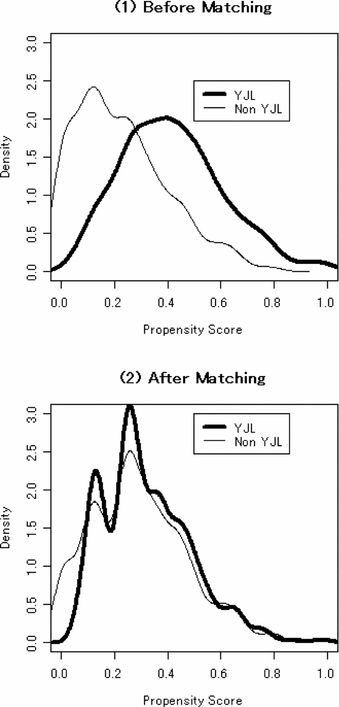
In order to summarize the balance of covariate distributions, we compare the distributions of propensity scores between YJL and non-YJL judges before and after matching. Propensity scores are predicted values of logistic analysis where we regress Leftist on all matched-on covariates, implying the probability that the observation is an YJL judge. When balance is achieved and a distribution of covariates is independent of Leftist, the distributions of propensity scores should not differ between the two judge groups. According to Figure 1, the distributions of propensity scores are considerably different before matching, while they are similar after matching. Clearly, the covariates are much better balanced after matching.

Figure 1. Distributions of propensity scores
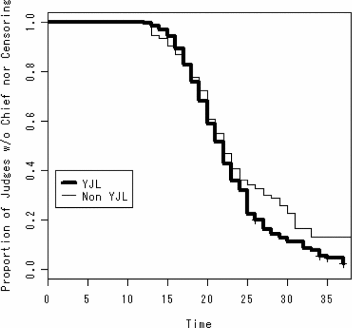
Figure 2 depicts the life tables. The survival curves are indistinguishable between the two groups up to the 25th year, while they differ after that. It is difficult to decide whether Leftist affects Time to division chief.
Figure 2. Comparison of life tables between the two judge groups (matched data)
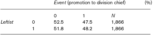
Table 3 cross-tabulates the percentage of Leftist and Event in the matched data. Using all 1,866 pairs, the average treatment effect of Leftist on Event is 0.007, while its standard error (estimated by using the central limitation theorem) is 0.015. Using uncensored 495 pairs only, the average treatment effect of Leftist on Time is 0.170, while its standard error is 0.274. Thus, both effects are not significant even at the 10% level and we cannot say that Leftist has any effect on Time to division chief or Event of promotion to division chief. In addition, even at the 10% significance level, a chi-square test with continuity correction also fails to reject the null hypothesis that Leftist does not matter whether judges are promoted to division chief before censoring. These results also suggest that Leftist does not shorten censoring time and proportions of judges on the promotion track are equal between the YJL group and the non-YJL group. The next subsection considers these points.
Table 3. Cross-tabulation of Leftist and Event (promotion to division chief) in matched data

Note: Chi-squared value continuity correction is 0.182. Since degree of freedom is 1, p-value is 0.670.
Survival analysis
Even if researchers use parametric modeling, it is much better to use matched data instead of raw data. This is because model dependence is reduced. Ho et al. (Reference Ho, Imai, King and Stuart2007) recommends that we use non-parametric matching as ‘preprocessing’, namely, a tool to remove bias of correlated control variables, before we perform any parametric analysis. We still rely on our survival model specification such as a log logistic distribution for latent time and the split population assumption, although we need not worry about which independent variables are included and whether they should be squared or interacted with other variables. Even if matching fails to balance these covariates completely, the parametric models can control them as long as they are correctly specified.
Table 4 reports the result of survival analysis of Time to division chief. We calculate standard errors and confidence intervals by bootstrapping the matched data, which is a little different from usual bootstrap. We resample the matched pairs, not the observations, with replacement in order to retain a balanced joint distribution of covariates between the two groups. We repeat this re-sampling 1,000 times, calculate standard deviances of 1,000 sets of parameter estimates in the survival analysis, and multiply them by 1000/(1000–1), which will be our unbiased estimates of standard errors. A 95% confidence interval is derived by 2.5% quantile value and 97.5% ones without assuming any distribution of estimates.
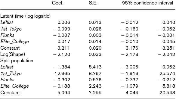
Table 4. Split population survival analysis of Time to division chief (matched data)
Notes: N = 3,732. The coefficients for cohort dummies are not reported. Standard error and 95% confidence interval are calculated by bootstrap. Log likelihood is –5646.294.
For the covariates in both latent time and split population models, we use the same independent variables introduced by Ramseyer and Rasmusen (Reference Ramseyer and Rasmusen2003). The coefficients of Leftist are significant in neither latent time part nor split population part. We cannot say that YJL membership matters either for whether judges are promoted to division chief or for whether they are on the promotion track. Thus, this parametric model of survival analysis reaffirms the irrelevance of YJL membership, which the non-parametric analysis of average treatment effects on Time and Event show in the previous subsection.
To briefly discuss the estimates for the control variables, 1st_Tokyo and Flunks fasten Time to division chief. Flunks also decreases the chance to be on the track to division chief.Footnote 20 Since Flunks is defined by the age of a judge starting her career, its estimates imply that those who took relatively long to become a judge may reach a division chief post earlier due to their age. We find that Elite_College is insignificant in both latent time part and split population part.
Conclusion
Is the Japanese judicial system independent of political control? Ramseyer and Rasmusen (Reference Ramseyer and Rasmusen2003) studied how long it takes for a judge to reach a division chief post, and argued that judges with leftist preferences do worse in their careers. This article shows that their analysis is problematic as it is based on inaccurate data; takes no account of the issues of censoring, left truncation, and split population; and depends critically on their model (mis-)specification. In this article, we corrected their data; we employed parametric survival analysis to deal with the issues of censoring, left truncation and split population, and we conducted matching to reduce model dependence and estimate non-parametric average treatment effects of YJL membership on time to, and occurrence of, promotion to division chief. As a result, we cannot find any evidence that YJL membership harms the judge's chances of reaching the post of division chief.
We interpret these findings as indicating either that leftist judges are independent and the government is not discriminating against them, or that they are dependent and the government need not to discriminate them. Moreover, if YJL affiliation damaged the judges’ career, it would imply that some judges were independent enough to resist and, thus, be discriminated against by, the government. In other words, judicial independence necessitates that the government acts to promote its followers and punishes those who protest its policies. On the contrary, in systems where the government controls the judiciary, judges may not express any conflict with the executive branch in the first place. Viewed in this light, other analyses in Ramseyer and Rasmusen (Reference Ramseyer and Rasmusen2003) which suggest that the government penalized recalcitrant judges, are all problematic. In short, however significant or insignificant the main coefficient is, their research design can never allow us to conclude that leftist judges are dependent. Given that the Japanese judicature is one of the allegedly-most dependent judiciary branches, we suggest that our findings should also cause scholars of comparative judicial politics to reconsider their measurements of judicial independence.
This article also aims to contribute to political methodology. Our new survival analysis model takes into consideration both left truncation and split population. Moreover, for the first time, we extend the causal inference literature to censored time-to-event data which have two dependent variables and propose a method of estimating the average treatment effects on time and event. Needless to say, our methods are not limited to application to judges in Japan. We offer two examples of where they may be applicable below.
One instance is length of legislative deliberation. How long does it take for bills to pass in the legislature? What is important to keep in mind when studying this is that some bills may not pass the legislature by the end of session (censoring: see Becker and Saalfeld, Reference Becker, Saalfeld, Doring and Hallerberg2004; Martin, Reference Martin2004; Masuyama, Reference Masuyama2001). Bills are introduced not only at the beginning of the session but also during the session (left truncation: Masuyama, Reference Masuyama2001). Moreover, some bills will never pass even if there is no end in the legislative session (split population).
Another promising application is to the democratic peace debate. Are democratic dyads less likely to fight than other dyads? There are several problems with the literature. One is that currently peaceful dyads may fight in the future (censoring). A second is that some dyads have no opportunities to fight (split population, Clark and Regan, Reference Clark and Regan2003). Other dyads fight several times (repeated events and left truncation).
In both examples, to reduce model dependence, matching is preferable. Thus, average treatment effects on time and event may help scholars to find rigorous causal effects. We believe that our analysis provides a good example of causal inference of censored time-to-event data for the students of both judicial politics and political methodology.
About the authors
Kentaro Fukumoto is Professor of Political Science at Gakushuin University and visiting fellow at Washington University in St Louis. He received his Ph.D. from University of Tokyo. His research interests include political methodology, legislative studies, and electoral studies. He is the author of Nihon no Kokkai Seiji: Zen Seifu Rippo no Bunseki [Politics in the Japanese Diet: A Statistical Analysis of Postwar Government Legislation] (Tokyo Daigaku Shuppan Kai, 2000) and Rippo no Seido to Katei [Legislative Institutions and Process] (Bokutaku Sha, 2007). His articles have appeared in American Political Science Review, American Journal of Political Science, Legislative Studies Quarterly, Journal of American Statistical Association, and Japanese Journal of Political Science.
Mikitaka Masuyama is Professor of Political Science at the National Graduate Institute for Policy Studies. He received his Ph.D. from the University of Michigan. His research interests include legislative institutions, Japanese politics and political methodology. He is the author of Gikai Seido to Nihon Seiji: Giji Un’ei no Keiryo Seijigaku [Agenda Power in the Japanese Diet: A Duration Analysis of Lawmaking] (Bokutakusha, 2003). His articles have appeared in Japanese Journal of Political Science, Journal of Legislative Studies and Social Science Japan Journal.