L-band radiometer design for long-term stability measurement of one-port devices

Emilie Leynia de la Jarrige; Laurent Escotte; Eric Gonneau; Jean-Marc Goutoule

doi:10.1017/S1759078711000997

L-band radiometer design for long-term stability measurement of one-port devices

Published online by Cambridge University Press: 14 December 2011

Emilie Leynia de la Jarrige ,

Laurent Escotte ,

Eric Gonneau and

Jean-Marc Goutoule

Show author details

Emilie Leynia de la Jarrige*: Affiliation:
LAAS CNRS, 7 avenue du colonel Roche, 31077 Toulouse, Cedex, France. Université de Toulouse; UPS, INSA, INP, ISAE; LAAS; F-31077 Toulouse, France.
Laurent Escotte: Affiliation:
LAAS CNRS, 7 avenue du colonel Roche, 31077 Toulouse, Cedex, France. Université de Toulouse; UPS, INSA, INP, ISAE; LAAS; F-31077 Toulouse, France.
Eric Gonneau: Affiliation:
SIMAD, Université de Toulouse, F-31077 Toulouse, France.
Jean-Marc Goutoule: Affiliation:
EADS Astrium, 31402 Toulouse, France.
*: Corresponding author: E. Leynia de la Jarrige Email: eleyniad@laas.fr

Article contents

Abstract
INTRODUCTION
EXPERIMENTAL SETUP
TEMPERATURE-STABILIZED SYSTEM
RADIOMETER CHARACTERISTICS
CONCLUSION
References

Rights & Permissions

Abstract

The design of a high-stability radiometer is presented in this paper. It is used to characterize the stability of a microwave active cold load at L-band. The two-load radiometer takes advantage of a noise injection technique to improve its sensitivity. A temperature-stabilized enclosure is used to minimize gain and noise temperature fluctuations of the receiver. The radiometer sensitivity is 0.031 K and the gain fluctuations are less than 0.005 dB during 1 day. The total gain and the receiver noise temperature of the radiometer exhibit very small variations (<0.03 dB and 1 K, respectively) on the long term.

Keywords

Radiometer Stability Gain fluctuations

Type: Research Papers
Information: International Journal of Microwave and Wireless Technologies , Volume 4 , Special Issue 1: IJMWT Special Issue on the 2011 National Microwave Days in France , February 2012 , pp. 119 - 126

DOI: https://doi.org/10.1017/S1759078711000997 [Opens in a new window]
Copyright: Copyright © Cambridge University Press and the European Microwave Association 2011

I. INTRODUCTION

Microwave radiometers are largely employed in several domains to measure electromagnetic radiations. Radio astronomy [Reference Tiuri1], Earth observation [Reference Ulaby2], human presence detection [Reference Nanzer and Rogers3], and industrial applications [Reference Borgarino, Polemi and Mazzanti4] are a few examples where radiometers play an important role and can be viewed as antenna–receiver systems. They are also used to characterize the noise behavior of linear one-port devices [Reference Wiatr and Schmidt-Szalowski5, Reference Randa, Billinger and Rice6] and microwave amplifiers [Reference Wait and Engen7]. In this case, the antenna is replaced with coaxial or waveguide structures to realize on-wafer measurements or to characterize connectorized devices. The measured powers are generally expressed in terms of equivalent temperatures for practical considerations (brightness temperature, antenna temperature, noise temperature, equivalent temperature, etc.). Several architectures of radiometers have been proposed during the last few decades [Reference Skou and Le Vine8]. The Total Power Radiometer (TPR) is the basic radiometer. The best sensitivity is obtained from the TPR, but frequent calibrations are required to minimize receiver gain and noise temperature instabilities. This problem is greatly alleviated with the Dicke Radiometer (DR) [Reference Dicke9]. A switch located at the receiver input associated with a synchronous detector is used to measure the difference between the antenna temperature (T _A) and the equivalent temperature of a known reference (T _Ref). The null-balancing DR corresponds to the case where T _Ref is equal to T _A [Reference Machin, Ryle and Vonberg10]. A variable noise source associated with a feedback control system is used to realize the above condition. The gain modulation radiometer is another type of receiver for obtaining balanced operation of the DR [Reference Tiuri1]. The Noise Adding Radiometer (NAR) does not require a switch at the receiver input [Reference Ohm and Snell11]. An excess noise level is periodically added to the antenna input signal with the help of a directional coupler. The problem of gain stability inherent to the TPR is then reduced with this architecture. The Noise Injection Radiometer (NIR) is a combination of the null-balanced DR and the NAR [Reference Goggins12]. The noise level (noise temperature, T _inj) added to the antenna signal is adjusted with a servo loop in order to meet T _inj + T _A = T _Ref. Excellent performance in terms of stability is achieved using the NIR at the expense of a loss of sensitivity. The Two-Load Radiometer (TLR) uses two reference temperatures and is continuously calibrated [Reference Hach13]. The resolution can be adjusted for a particular measurement problem and different designs are proposed and analyzed in [Reference Goodberlet and Mead14]. The Correlation Radiometer (CR) is composed of two identical radiometers with separate antennas and has been discussed in several works [Reference Blum15, Reference Fujimoto16]. Two different sources can be simultaneously observed and their cross-correlation is determined with a complex correlator. The CR is easily adapted for use in an interferometer system. A modified version, the so-called pseudo correlation radiometer, is employed in the Planck low-frequency instrument for measuring the anisotropy of the cosmic microwave background [Reference Aja17].

The choice of the radiometer will mainly depend on the final application. The constraints for calibrating the instrument or concerning the measurement time are not necessarily the same if the radiometer is a ground-based system, a microwave aircraft instrument, or a space system. For example, the CR is well adapted to measure the ocean brightness temperature, each antenna measuring two different polarizations, but is not appropriate to measure the stability of a one-port device. The calibration of radiometers is realized by measuring different sources with well-known equivalent temperatures. A cold source is generally needed and several types can be found [Reference Skou and Le Vine8]. A cooled microwave load is the simplest way. Antenna target calibration is another solution where the cold source could be either a microwave absorber soaked with liquid nitrogen, or the cold sky. Active devices have been also proposed to realize a matched load with a low noise temperature, also called Active Cold Load (ACL). The first ACL realized with a single GaAs Field Effect Transistor (FET) with appropriate feedback was proposed in the 1980s by Frater and Williams [Reference Frater and Williams18]. A noise temperature around 50 K at L-band was reported by the authors. We have presented in a previous paper that a SiGe heterojunction bipolar transistor (HBT) can also be used to realize an ACL at L-band [Reference Leynia de la Jarrige, Escotte, Goutoule, Gonneau and Rayssac19]. A noise temperature T _n less than 65 K, a return loss higher than 30 dB and a temperature-sensitivity around 0.3 K/°C are the main characteristics of the proposed ACL. The stability of this kind of load is a key parameter for space-borne radiometers and this parameter must be evaluated on the long term. A dedicated radiometer has been developed to characterize the ACL long-term stability. It was described in a previous paper related to the stability analysis of the SiGe ACL [Reference Leynia de la Jarrige, Escotte, Gonneau and Goutoule20]. We will present in this paper additional information concerning some practical considerations on the radiometer design, and an in-depth analysis concerning the temperature regulation of the test-bed. The radiometer gain stability is particularly detailed. Gain fluctuations are examined on the long term and the different types of low-frequency noise sources are determined from the normalized gain spectrum.

II. EXPERIMENTAL SETUP

A) Radiometer architecture

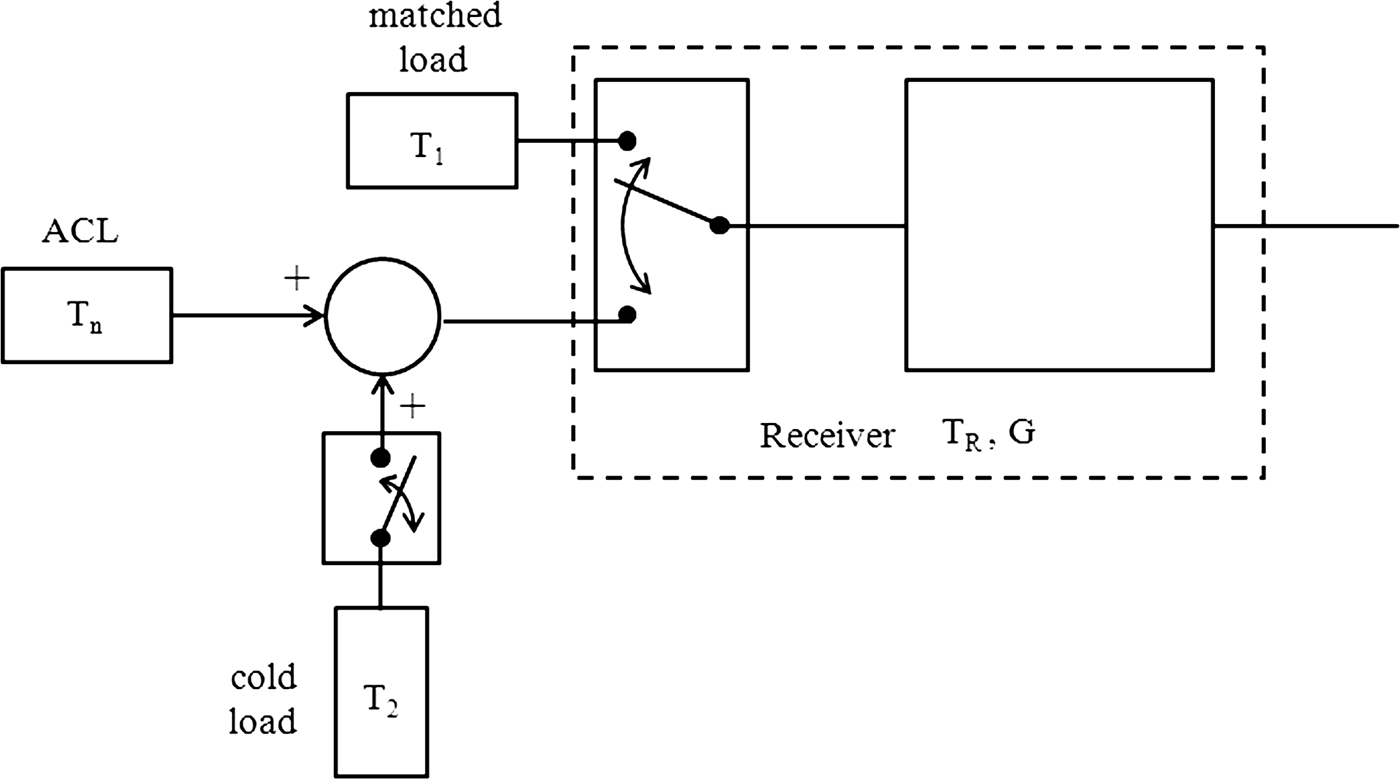
The architecture of the test-bed is based on the two-load radiometer and is represented in Fig. 1. It resembles the NIR one, except that the injected noise value is fixed to a constant value. The two reference loads (T ₁ and T ₂) can be shown in the simplified block-diagram depicted in Fig. 2 [Reference Goodberlet and Mead14]. T ₁ corresponds to the physical temperature of the matched load (“hot load”) and T ₂ is the “cold load” realized with both the calibration noise diode and 16-dB directional coupler. The latter is also used for the addition. The single-throw switch is represented in Fig. 2 to symbolize the bias command of the calibration noise diode. The value of T ₂ is chosen to fulfill T _n + T ₂ as close as possible to T ₁. This significantly improves the sensitivity of the instrument as will be shown in the next paragraph. The coaxial switch (the first receiver element) features very low insertion loss (0.04 dB) and an isolation value higher than 120 dB at L-band. Its reliability is a critical parameter since long-term stability is investigated over several months. Insertion loss repeatability is specified to be better than 0.03 dB for 5 million cycles. This corresponds to 10 switching per minute over 1 year. The low-noise amplifier (LNA) is the second element of the receiver and sets the receiver sensitivity. It is a commercially available amplifier (AMF-4F from Miteq). The noise figure is 0.45 dB at 25°C and the power gain G _p is higher than 60 dB at L-band. The dissipated power by the LNA is around 3.75 W and it acts as a heating element into the radiometer. The frequency bandwidth of the three-pole cavity Band-Pass Filter (BPF) is the same as the one of the ACL (1400–1427 MHz). The transmission coefficient of the LNA and the BPF was measured at 25°C with a network analyzer and we have found a maximum value of 61.4 dB and a ripple less than 0.15 dB in the frequency band of interest. The equivalent noise bandwidth B _n calculated from the measured data using numerical integration is 60 MHz. These values are well adapted to obtain incident noise powers between −40 and −35 dBm, ensuring a quadratic behavior of the microwave detector. In this case, the output voltage of the detector is proportional to the incident noise power, and then to the incident noise temperature. The detector is a Tunnel detector, with a responsivity R _d around 1 mV/μW at 25°C and a low level of noise (2 nV/√Hz at 100 Hz). The video output exhibits a low resistance value (<320 Ω) and a capacitance of 400 pF. The square-law detector is followed by a commercially available dc amplifier (model 351A from Analog Modules Inc.), which has 80-dB voltage gain (G _v). This value is necessary to amplify the detected voltage to an acceptable level required for the analog–digital converter. The noise floor of the amplifier is less than 1 nV/√Hz and the noise bandwidth of the video output is reduced with the help of the low-pass filter (simple RC circuit) which has a typical time constant value of 5 ms [Reference Skou and Le Vine8].

Fig. 1. Block-diagram of the experimental setup. The red marks on the microwave circuits correspond to the thermistors.

Fig. 2. Simplified block diagram of the two-load radiometer.

The choice of the radiometer architecture was guided by two considerations: the test bed stability is realized with frequent calibrations and the injected noise value can be controlled. The incident noise powers on the detector and the output voltages are then in the same range. The problems related to the detector non-linearity are then minimized and the analog–digital converter operates in the same range. The design of the test bed has been also realized in part with the help of low-frequency (LF) noise measurements. The receiver and video parts were assembled at room temperature (without temperature regulation) and several types of detectors (Schottky, Tunnel) have been tested with a vector signal analyzer (Hp 89410A). The best solution in terms of LF noise, and then in terms of stability, was selected taking into account the assembly of the different circuits in the system and more particularly the association between the microwave detector and the dc amplifier.

B) Radiometer equations

The measurement cycle is depicted in Fig. 3. The output voltage V ₀ is measured during τ ₀ when the microwave switch is connected to the matched load. For the other switch position, the output voltage V ₁ is measured during τ ₁ when the calibration noise diode is off and the output voltage V ₂ is measured during τ ₂ when the calibration noise diode is on. The corresponding equations are follows:

(1)

$V_0=R_{\rm d} G_{\rm v} kG_{\rm p} B_{\rm n} \lpar T_{\rm R}+T_{{\rm a}1} \rpar \comma$

(2)

$V_1=R_{\rm d} G_{\rm v} kG_{\rm p} B_{\rm n} \lpar T_{\rm R}+T_{{\rm oc}1} \rpar \comma$

(3)

$V_2=R_{\rm d} G_{\rm v} kG_{\rm p} B_{\rm n} \lpar T_{\rm R}+T_{{\rm oc}2} \rpar \comma$

where k is Boltzmann's constant (1.38 × 10⁻²³ J/K) and T _R is the receiver noise temperature. R _d corresponds to the responsitivity of the detector (in V/W) and T _a1 is the physical temperature of the matched load. T _oc1 and T _oc2 are the noise temperatures at the output of the directional coupler when the calibration noise diode is off and on, respectively, and are given by the noise theory of linear multiport [Reference Wait21]:

(4)

$T_{{\rm oc}1}=\displaystyle{{T_{\rm n} } \over L}+N_{{\rm int}}+\displaystyle{{T_{{\rm a}2} } \over C}\comma$

(5)

$T_{{\rm oc2}}=\displaystyle{{T_{\rm n} } \over L}+N_{{\rm int}}+\displaystyle{{T_{\rm h} } \over C}\comma$

where L and C are the loss and coupling values of the coupler. These values have been determined at several physical temperatures from S-parameter measurements carried out in a temperature-regulated chamber. T _n is the ACL noise temperature. T _a2 and T _h are the physical temperature of the calibration noise diode in the off state, and the noise temperature of the calibration noise diode in the on state, respectively. N _int is the internal noise of the coupler at physical temperature T _a3, given by [Reference Wait21]:

(6)

$N_{{\rm int}}=\left({1 - \displaystyle{1 \over L} - \displaystyle{1 \over C}} \right)T_{{\rm a}3} .$

The physical temperatures of the different microwave passive circuits are different in the previous equations due to the presence of a temperature gradient inside the radiometer mainly produced by the LNA. Equations (1)–(6) are the same as those given in [Reference Leynia de la Jarrige, Escotte, Goutoule, Gonneau and Rayssac19] if the physical temperatures are supposed to be constant. The expressions of T _n, T _R, and the total gain G of the radiometer are obtained by combining (1)–(6):

(7)

$T_{\rm n}=L \times \left({T_{{\rm a}1} - T_{{\rm a3}}+\displaystyle{{T_{{\rm a}3} } \over L}+\displaystyle{{T_{{\rm a3}} - T_{{\rm a}2} } \over C}} \right)- \displaystyle{L \over C} \times \displaystyle{{V_0 - V_1 } \over {V_2 - V_1 }} \times \lpar T_{\rm\comma } - T_{{\rm a}2} \rpar \comma$

(8)

$T_{\rm R}=\displaystyle{{V_0 } \over {V_2 - V_1 }} \times \displaystyle{{T_{\rm h} - T_{{\rm a2}} } \over C} - T_{{\rm a1}}\comma$

(9)

$G=G_{\rm v} G_{\rm p}=\displaystyle{C \over {R_{\rm d} kB_{\rm n} }} \times \displaystyle{{V_2 - V_1 } \over {T_{\rm h} - T_{{\rm a2}} }}.$

The ACL noise temperature given by (7) can be expressed in the compact form:

(10)

$T_{\rm n}=T_x - T_y \times \gamma .$

Fig. 3. Typical measurement cycle.

T _x corresponds to the first term in (7) and is close to the ambient temperature of the radiometer since T _a1, T _a2, and T _a3 are only slightly different. T _y is another constant depending on the noise injection circuitry (L, C, T _h, and T _a2) and γ is related to the measured voltages:

(11)

$T_y=L \times \left({\displaystyle{{T_{\rm h} - T_{{\rm a2}} } \over C}} \right)\comma$

(12)

$\hskip-2.5pc\gamma=\displaystyle{{V_0 - V_1 } \over {V_2 - V_1 }}.$

According to the mathematical analysis given in [Reference Goodberlet and Mead14], the noise-equivalent delta temperature (NEDT), corresponding to the standard error ΔT _n, can be expressed as

(13)

$\Delta T_{\rm n}=T_y \times \sqrt {\Delta V_0 ^2 \left({\displaystyle{{\partial \gamma } \over {\partial V_0 }}} \right)^2+\Delta V_1 ^2 \left({\displaystyle{{\partial \gamma } \over {\partial V_1 }}} \right)^2+\Delta V_2 ^2 \left({\displaystyle{{\partial \gamma } \over {\partial V_2 }}} \right)^2 } .$

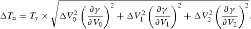
ΔV ₀², ΔV ₁², and ΔV ₂² are the variances associated with the measurement errors of V ₀, V ₁, and V ₂, respectively. These variances depend on the different integration times (τ ₀, τ ₁, and τ ₂) and optimum values of these parameters can be experimentally determined as will be shown in Section IV. The expressions of the derivatives in (13) can be easily derived from (12):

(14)

$\displaystyle{{\partial \gamma } \over {\partial V_0 }}=\displaystyle{1 \over {V_2 - V_1 }}\comma$

(15)

$\displaystyle{{\partial \gamma } \over {\partial V_1 }}=\displaystyle{{V_0 - V_2 } \over {\lpar V_2 - V_1 \rpar ^2 }}\comma$

(16)

$\displaystyle{{\partial \gamma } \over {\partial V_2 }}=\displaystyle{{V_1 - V_0 } \over {\lpar V_2 - V_1 \rpar ^2 }}.$

It is clear from (11) and (13) that a low loss coupler is desired to minimize the measurement error. Equation (13) can also be minimized if (15) is equal to 0, i.e. if V ₀ is close to V ₂. This corresponds to the condition T ₁ = T _n + T ₂ reported in the previous paragraph and is realized by a proper choice of T _h and C.

C) Data acquisition and system control

A multifunction data acquisition (DAQ) device (Agilent U2351A) realizes the connection between the computer and radiometer (Fig. 1). A graphical user interface was coded with Matlab for the radiometer control and for the signal processing. A digital signal is generated by the DAQ and is sent to a command circuit used for demultiplexing the pulse waveform signal. The latter generates three different signals that control the switch position and the calibration noise diode bias to realize the measurement cycle depicted in Fig. 3. Synchronized analog–digital conversion of both the output voltage and signals from the different thermistors is performed at a sampling rate of 7 kHz. The data are stored in the DAQ memory and are transferred to the computer at the end of the measurement cycle through a universal serial bus (USB) high-speed connection. Data processing is realized in real time. The different output voltage values (V ₀, V ₁, and V ₂) are extracted from the measured signal and are averaged over their corresponding integration times. The ACL noise temperature, receiver noise temperature and total gain of the radiometer are derived from (7) to (9). The different physical temperatures (T _a0 to T _a4) are also calculated from the thermistors characteristics and the measured voltages at their terminals. The main parameters are then displayed in real time and the relevant data are stored.

III. TEMPERATURE-STABILIZED SYSTEM

Microwave circuits are temperature-sensitive elements and a thermal control is required to improve the radiometer stability. Several methods can be found to keep the temperature at a constant value. For environmental parameter measurements where the instrument is exposed to important temperature variations, it is generally useful to place the RF front-end in a separated, insulated, and regulated box. The RF section can either be heated or cooled, the latter solution being used in radio-astronomy to reduce the receiver noise temperature. Using an auxiliary temperature control method, Kemppainen et al. report that the front-end temperature is stabilized to ±0.06°C and the L-band radiometer performances are improved by keeping the RF front-end very close to the antenna feeds [Reference Kemppainen22]. Temperature variations within ±0.02°C around 47.2°C are reported by Lemaître et al. for the RF section regulated with heating resistors of a ground-based L-band radiometer [Reference Lemaître23]. Tanner uses a thermoelectric cooler to reach an ultra-stable temperature of 35 ± 0.004°C for a Ka-band radiometer [Reference Tanner24]. A dedicated radiometer for ACL stability measurements at X-band is proposed in [Reference Sobjaerg, Skou and Balling25]. A thermal stability of the microwave section better than 0.02°C for a 15°C change in ambient temperature is reported by the authors. For these few examples, the temperature of the RF section is then accurately controlled and stabilized and the temperature of the other part of the radiometer is also regulated to a lesser extent. The air inside the other part of the radiometer is generally continuously stirred by one or several fans.

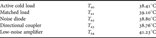
Our measurement system is located in a temperature-regulated room (22 ± 1°C). The radiometer design is then simplified: all the elements (shown in Fig. 1) are mounted in the same insulated enclosure. A 10-mm-thick aluminum box (400 × 300 × 100 mm) is covered by a 40-mm-thick extruded polystyrene layer, as shown in Fig. 4. Heating resistors are fixed on the bottom plate and are controlled by a dedicated temperature control circuit [Reference Barillet, Viennet, Petit and Audoin26]. Figure 5 represents the simplified block-diagram of the circuit. The Wheatstone bridge is composed of two thermistors (R _t) and two precision resistors (R _p). The voltage at the amplifier output is proportional to the difference between R _t and R _p. The oscillator stage is an operational amplifier operating as a multi-vibrator when the value of R _t is close to that of R _p. The power stage is composed of two transistors operating in switching mode. The first one sets the current value in the load, corresponding to the heating resistors. The cycle ratio of the multi-vibrator is variable (when R _t is close to R _p) and depends on the difference between R _t and R _p (i.e. the difference between the thermistor temperature in the Wheatstone bridge and the desired temperature fixed by R _p). At the startup, the value of R _t is higher than R _p and the second transistor in the power stage is always saturated and the maximum power is dissipated in the heating resistors. Several thermistors located on several microwave circuits (see the red marks in Fig. 1) are used to monitor the temperature inside the radiometer. We can see in Table 1 that the temperature is not uniform. This is mainly due to the low-noise amplifier and its own dissipated power. The ACL is the farthermost element of the LNA and it exhibits the lowest temperature. The temperature values reported in Table 1 correspond to mean values recorded during 4 days. The standard and maximum deviations are less than 0.002 and 0.01°C, respectively. Long-term stability measurements of the ACL were realized during 138 days from October 2010 to February 2011. Figure 6 represents the variations of the ACL physical temperature during this period. Each point corresponds to the mean value calculated during 1 day (about 875 points) and the error bars are related to the confidence interval of ±σ (σ is the standard deviation). The temperature deviation during more than 4 months is less than 0.04°C. A peak appears (well marked on the standard deviation) around the 100th day due to a trouble in the air-conditioning of the room. The measurements have been stopped after 30 and 60 days due to problems in the radiometer command circuit. The mean value of the standard deviation is 0.0015°C, corresponding to a typical temperature fluctuation less than 0.01°C over 1 day.

Fig. 4. Photograph of the temperature-stabilized system.

Fig. 5. Simplified block-diagram of the temperature control circuit.

Fig. 6. ACL physical temperature versus time recorded from October 1, 2010 to February 15, 2011. The errors bars correspond to ±σ.

Table 1. Temperature of microwave circuits inside the radiometer.

IV. RADIOMETER CHARACTERISTICS

The main radiometer characteristics are determined with a dedicated program developed for that purpose. The different output voltages (V ₀, V ₁, and V ₂) are continuously measured during 150 min when the switch and the calibration noise diode bias are in their corresponding states. Allan variance, or two-sample variance, is used to analyze the voltage variations versus time. This statistical tool was proposed in the 1960s to study the stability of frequency sources [Reference Allan27] and was also used to investigate radiometer stability [Reference Rau, Schieder and Vowinkel28] and many other parameters in different scientific fields. An estimate of the Allan variance (σ_AV²) is given by [Reference Rutman29]:

(17)

$\sigma _{{\rm AV}}^2=\displaystyle{1 \over {2\lpar n - 1\rpar }}\sum\limits_{i=1}^{n - 1} {\lpar \bar V_{i+1} - \bar V_i \rpar ^2 } .$

n represents the number of data (or time slots) used to estimate the variance and corresponds to the averaged value of the output voltage during the integration time interval τ. The plot of σ_AV² versus τ is reported in Fig. 7 for the different output voltage values. The value of n decreases when τ increases. A minimum value of 64 time slots is used to derive σ_AV² at 70 s. The solid lines correspond to the simple model given by:

(18)

$\sigma _{{\rm AV}}^2=\displaystyle{{A_{ - 2} } \over {\tau ^2 }}+\displaystyle{{A_{ - 1} } \over \tau }+A_0+A_1 \tau .$

Fig. 7. Allan variance versus integration time. The solid lines correspond to the model given by (18).

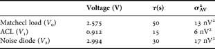
A ₋₂, A ₋₁, A ₀, and A ₁ are fitting parameters. We can see in Fig. 7 that the variance decreases when the integration time grows due to a reduction of the white noise in the measurement set-up. However, the value of τ cannot be infinitely increased since additional fluctuations appear. We observe a plateau above 15 s for the ACL measurement, which is attributed to flicker noise or 1/f noise. The same behavior is observed for the matched load characterization above 50 s. Concerning the calibration noise diode measurement, a minimum occurs in the plot of the Allan variance. For integration time values higher than 30 s, σ_AV² increases against τ, which corresponds to the presence of a 1/f ² noise source [Reference Rutman29]. This additional noise source is attributed to the calibration noise diode in the on state and could be attributed to random walk noise, generation–recombination noise or burst noise with very long time constants. The integration time values have been selected from Fig. 7 to minimize the NEDT in the data processing. Typical values of output voltages, integration times, and Allan variances are reported in Table 2. The NEDT, or sensitivity, can be calculated from (13)–(16) with the data given in Table 2, assuming that ΔV ² = 2σ_AV² [Reference Rau, Schieder and Vowinkel28] and we found a value of 0.031 K. The magnitude of each contribution term in (13) can be evaluated. We found that the highest contribution is mainly due to the measurement of the matched load (54% of the total value under the square root of (13)), whereas the error associated with the ACL measurement represents only 1%.

Table 2. Radiometer characteristics determined from Allan variance analysis.

The receiver gain instabilities are a limiting factor in radiometric measurements. The total gain of the radiometer given by (9) must be particularly stable during the total integration time (τ ₀ + τ ₁ + τ ₂) corresponding to the measurement cycle. Figure 8 represents its variations versus time recorded during the ACL long-term stability measurement. The points correspond to the mean values calculated during 1 day (about 875 measurements) and the error bars are related to the confidence interval of ±σ. Two distinct behaviors can be observed. In the first step, the gain slightly increases. After the second break (a discrete transistor was changed in the command circuit), the gain is stabilized and the maximum deviation is less than 0.007 dB. The mean value of the standard deviation is less than 0.001 dB, which indicates that the gain fluctuations are less than 0.005 dB over 1 day. The presence of low-frequency noise sources in the measurement was also investigated during about 1 week, in the period corresponding to the vertical dotted lines in Fig. 8. A sample of more than 5000 points, recorded from December 24 to December 30, 2010, has been used to evaluate the gain stability of the test set. The Power Spectral Density (PSD) of the low-frequency gain fluctuations S _G(f) was calculated from discrete Fourier transform (512 points are used and the PSD is an average of 9 spectra). The normalized value (ΔG/G) is obtained by dividing the square root of S _G(f) by the mean value of G. The variations of ΔG/G versus frequency are reported in Fig. 9. A simple model given by (19) is also plotted.

(19)

$\displaystyle{{\Delta G} \over G}=k_0+\displaystyle{{k_1 } \over {f^\alpha }}=1.1 \times 10^{ - 3}+\displaystyle{{2.5 \times 10^{ - 6} } \over {f^{0.75} }}$

Fig. 8. Total gain of the radiometer versus time recorded from October 1, 2010 to February 15, 2011. The errors bars correspond to ±σ. The vertical dotted lines indicate the period where the normalized gain fluctuation spectrum plotted in Fig. 9 is calculated.

Fig. 9. Normalized gain fluctuation of the radiometer versus frequency. The solid line corresponds to the model given by (19).

The value of k ₁ is generally used to compare the stability of different low-noise amplifiers [Reference Wollack and Pospieszalski30]. The frequency index value (α = 0.75) indicates that S _G(f) is a combination of 1/f and 1/f ² noise sources. We can see in Fig. 9 that these excess noise sources become dominant below 1 mHz, which corresponds to a time period of 1000 s (largely higher than the total integration time). The small value of k ₁, associated with a small corner noise frequency value (0.3 mHz), indicate that the test set is very stable.

The receiver noise temperature is also very stable. A maximum deviation less than 1 K is observed during the whole period of the experiment. Typical variations less than 0.4 K during 1 day are also determined from statistical analysis. The long-term stability measurements of the SiGe HBT-based active cold load indicate that this kind of load is very stable. A maximum deviation less than 0.35 K was obtained over 4 months and a half corresponding to a stability of 0.8 K/year [Reference Leynia de la Jarrige, Escotte, Gonneau and Goutoule31].

V. CONCLUSION

We have presented in this paper the design of a radiometer dedicated to the stability measurement of one-port devices at L-band. Absolute accuracy was not addressed in this work, which simplifies the architecture of the test-bed. Noise injection technique is used with the two-load radiometer to improve its sensitivity. A temperature-stabilized system was developed to reduce the gain and noise fluctuations of the receiver which are found very stable on the long term. The sensitivity of the instrument is 0.031 K and the gain fluctuations are less than 0.005 dB during 1 day.

ACKNOWLEDGEMENT

This work was supported by the regional council of Midi-Pyrénées.

Emilie Leynia de la Jarrige was born in Angers, France, in 1985. She received the M.S. degree in electronics from the University of Rennes, Rennes, France; in 2008, and is currently working toward the Ph.D. degree in electronics at the Laboratoire d'Analyse et d'Architecture des Systèmes du Centre National de la Recherche Scientifique (LAAS-CNRS), Toulouse, France. Her main field of interest is in the study of noise in microwave devices and circuits, more particularly, ACL based on transistors for microwave radiometer calibration, and the development of dedicated radiometer to evaluate its stability.

Laurent Escotte was born in Nouméa, France, in 1962. He received the Ph.D. degree in optic and microwave communications from the University of Limoges, Limoges, France; in 1988. Since 1989, he has been an assistant professor of electronic engineering with the University Paul Sabatier, Toulouse, France. At the same time, he joined the Laboratoire d'Analyse et d'Architecture des Systèmes du Centre National de la Recherche Scientifique (LAAS-CNRS), Toulouse, France. Since 1999, he has been a professor of electronic engineering with the University Paul Sabatier. He has authored or co-authored over 50 technical papers. His current research interests include noise characterization and modeling of active devices and circuits in the microwave and millimeter-wave frequency range.

Eric Gonneau was born in Saint Pierre, Réunion Island, France, in 1965. He received the Ph.D. degree in signal processing from the Toulouse National Polytechnic Institute (INPT), Toulouse, France; in 1993. Since 1994, he has been an assistant professor of electronic engineering with the University Paul Sabatier, Toulouse, France. Until 2004, he was with the Laboratoire d'Acoustique de Métrologie et d'Instrumentation (LAMI), where he specialized in sources localization using array processing and active noise reduction on multiple-input–output systems. He is now with the Simulation Instrumentation et Matériaux pour l'Analyse Dosimétrique (SIMAD). He has authored or co-authored over 30 technical papers. His current research interests are noise fluctuations, digital signal processing, and image segmentation.

Jean-Marc Goutoule Jean-Marc Goutoule was born in Toulouse, France, in 1953. He received from the Institut National Polytechnique de Toulouse his Engineer degree in Electronics in 1976 and his “Habilitation á Diriger des Recherches” in 2008. He received his Doctor Engineer degree from ENSAE in 1979. Since 1979 he has performed Researches and Development in advanced microwave equipment and systems within Thomson CSF, Alcatel Espace and Matra Espace. Since 2000 he heads within Astrium a microwave group focused on space borne radiometers from L band interferometers up to sub-millimeter imagers. He has authored or coauthored over 30 technical paper.

References

REFERENCES

[1]Tiuri, M.E.: Radio astronomy receivers. IEEE Trans. Antennas Propag., 12 (1964), 930–938.CrossRef Google Scholar

[2]Ulaby, F.T.: Passive microwave remote sensing of the earth's surface. IEEE Trans. Antennas Propag., 24 (1976), 112–115.CrossRef Google Scholar

[3]Nanzer, J.A.; Rogers, R.L.: Human presence detection using millimeter-wave radiometry. IEEE Trans. Microw. Theory Tech., 55 (2007), 2727–2733.CrossRef Google Scholar

[4]Borgarino, M.; Polemi, A.; Mazzanti, A.: Low-cost integrated microwave radiometer front-end for industrial applications. IEEE Trans. Microw. Theory Tech., 57 (2009), 3011–3018.CrossRef Google Scholar

[5]Wiatr, W.; Schmidt-Szalowski, M.: The multistate radiometer: a novel means for impedance and noise temperature measurement. IEEE Trans. Instrum. Meas., 46 (1997), 486–489.CrossRef Google Scholar

[6]Randa, J.; Billinger, R.L.; Rice, J.L.: On-wafer measurements of noise temperature. IEEE Trans. Instrum. Meas., 48 (1999), 1259–1269.CrossRef Google Scholar

[7]Wait, D.; Engen, G.F.: Application of radiometry to the accurate measurement of amplifier noise. IEEE Trans. Instrum. Meas., 40 (1991), 433–437.CrossRef Google Scholar

[8]Skou, N.; Le Vine, D.: Microwave Radiometer Systems: Design and Analysis, 2nd ed., Artech House Boston/London, 2006.Google Scholar

[9]Dicke, R.H.: The measurement of thermal radiation at microwave frequencies. Rev. Sci. Instrum., 17 (1946), 268–275.CrossRef Google Scholar PubMed

[10]Machin, K.E.; Ryle, M.; Vonberg, D.D.: The design of an equipment for measuring small radio-frequency noise powers. Proc. IEE Part III, 99 (1952), 127–134.Google Scholar

[11]Ohm, E.A.; Snell, W.W.: A radiometer for a space communication receiver. Bell Syst. Tech. J., 42 (1963), 2047–2080.CrossRef Google Scholar

[12]Goggins, W.B.: A microwave feedback radiometer. IEEE Trans. Aerosp. Electron. Syst., 3 (1967), 83–90.CrossRef Google Scholar

[13]Hach, J.P.: A very sensitive airborne microwave radiometer using two reference temperatures. IEEE Trans. Microw. Theory Tech., 9 (1968), 629–636.CrossRef Google Scholar

[14]Goodberlet, M.A.; Mead, J.B.: Two-load radiometer precision and accuracy. IEEE Trans. Geosci. Remote Sens., 44 (2006), 58–67.CrossRef Google Scholar

[15]Blum, E.J.: Sensibilité des radiotélescopes et récepteurs à corrélation. Ann. Astrophys., 22 (1959), 140–163.Google Scholar

[16]Fujimoto, K.: On the correlation radiometer technique. IEEE Trans. Microw. Theory Tech., 12 (1964), 203–212.CrossRef Google Scholar

[17]Aja, B. et al. : Very low-noise differential radiometer at 30 GHz for the PLANCK LFI. IEEE Trans. Microw. Theory Tech., 53 (2005), 2050–2062.CrossRef Google Scholar

[18]Frater, R.H.; Williams, D.R.: An active cold noise source. IEEE Trans. Microw. Theory Tech., 29 (1981), 344–347.CrossRef Google Scholar

[19]Leynia de la Jarrige, E.; Escotte, L.; Goutoule, J.M.; Gonneau, E.; Rayssac, J.: SiGe HBT-based active cold load for radiometer calibration. IEEE Microw. Wirel. Compon. Lett., 20 (2010), 238–240.CrossRef Google Scholar

[20]Leynia de la Jarrige, E.; Escotte, L.; Gonneau, E.; Goutoule, J.M.: Stability analysis of an SiGe HBT-based active cold load. IEEE Trans. Microw. Theory Tech., 59 (2011), 354–359.CrossRef Google Scholar

[21]Wait, D.F.: Thermal noise from a passive linear multiport. IEEE Trans. Microw. Theory Tech., 16 (1968), 687–691.CrossRef Google Scholar

[22]Kemppainen, S. et al. : Thermal stabilized front-end PCB with active cold calibration load for L-band radiometer, in IEEE Int. Geoscience and Remote Sensing Symp., Barcelona, 2007, 4433–4436.Google Scholar

[23]Lemaître, F. et al. : Design and test of the ground-based L-band radiometer for estimating water in soils (LEWIS). IEEE Trans. Geosci. Remote Sens., 42 (2004), 1666–1676.CrossRef Google Scholar

[24]Tanner, A.B.: A high stability Ka-band radiometer for tropospheric water vapor measurements, in IEEE Aerospace Conf., Big Sky, Montana, 2001, 1849–1863.Google Scholar

[25]Sobjaerg, S.S.; Skou, N.; Balling, J.E.: Measurements on active cold loads for radiometer calibration. IEEE Trans. Geosci. Remote Sens., 47 (2009), 3134–3139.CrossRef Google Scholar

[26]Barillet, R.; Viennet, J.; Petit, P.; Audoin, C.: Circuit for temperature control. J. Phys. E: Sci. Instrum., 8 (1975), 544–545.CrossRef Google Scholar

[27]Allan, D.W.: Statistics of atomic frequency standards. Proc. IEEE, 54 (1966), 221–230.CrossRef Google Scholar

[28]Rau, G.; Schieder, R.; Vowinkel, B.: Characterization and measurement of radiometer stability, in 14th European Microwave Conf., Liège, 1984, 248–253.CrossRef Google Scholar

[29]Rutman, J.: Characterization of phase and frequency instabilities in precision frequency sources: fifteen years of progress. Proc. IEEE, 66 (1978), 1048–1075.CrossRef Google Scholar

[30]Wollack, E.J.; Pospieszalski, M.W.: Characteristics of broadband InP millimeter-wave amplifiers for radiometry, in IEEE MTT-S Int. Microwave Symp. Digest, Baltimore, 1998, 669–672.Google Scholar

[31]Leynia de la Jarrige, E.; Escotte, L.; Gonneau, E.; Goutoule, J.M.: Long-term stability of an SiGe HBT-based active cold load, in IEEE Int. Geoscience And Remote Sensing Symp., Vancouver, 2011, 3839–3842.CrossRef Google Scholar