


1 Introduction
When a supersonic jet is operating at off-design conditions, a train of quasi-periodic shock cells appears. Compared to subsonic or perfectly expanded supersonic jets, these shock cells lead to an additional kind of aerodynamic noise. Shock-cell noise is comprised of discrete tones (known as screech) and a broadband component. The generation of screech is due to a self-sustaining feedback loop (Powell Reference Powell1953) and is believed to be produced between the second and fourth shock cells (Edgington-Mitchell et al. Reference Edgington-Mitchell, Oberleithner, Honnery and Soria2014). The production of broadband shock-associated noise (hereafter BBSAN) follows a similar process (Tam, Seiner & Yu Reference Tam, Seiner and Yu1986), but without the resonant feedback loop.
The broadband component is generated by the interaction of downstream-travelling flow structures with the shock cells (Harper-Bourne & Fisher Reference Harper-Bourne and Fisher1973). This interaction produces sound waves that propagate to the far field, whose maximum intensity is in a direction perpendicular to the jet axis. In the far field, BBSAN is characterised by a broad spectral peak whose peak frequency is a function of the nozzle pressure ratio (NPR), convection velocity and observer location. The amplitude of BBSAN is dependent on the off-design parameter
 $\unicode[STIX]{x1D6FD}=\sqrt{M_{j}^{2}-M_{d}^{2}}$
where
$\unicode[STIX]{x1D6FD}=\sqrt{M_{j}^{2}-M_{d}^{2}}$
where
 $M_{j}$
and
$M_{j}$
and
 $M_{d}$
are the perfectly expanded and design Mach numbers of the jet, respectively.
$M_{d}$
are the perfectly expanded and design Mach numbers of the jet, respectively.
Models for BBSAN were initially developed based on experimental observations, such as the empirical model of Harper-Bourne & Fisher (Reference Harper-Bourne and Fisher1973) which is based on a phased array of localised sources along the jet centreline. The directivity of BBSAN is proposed to be due to the relative phasing between the sources, where the time delay in acoustic emission between adjacent sources is a function of the convection velocity of the convecting flow structures. While the model is capable of reproducing many of the acoustic far-field features, it incorrectly predicts the occurrence of harmonically related peaks, nor does it account for azimuthal modes other than the axisymmetric mode.
More recently semi-empirical hybrid models have been developed. With the increase in computational power available in recent times, hybrid models are now being used to model BBSAN for different nozzle geometries (Miller & Morris Reference Miller and Morris2010; Morris & Miller Reference Morris and Miller2010) with reasonable success. These models use Reynolds averaged Navier–Stokes (RANS) mean-flow solutions to provide input for acoustic-analogy source terms which link flow-field fluctuations to the propagation of sound waves in the far field (Lighthill Reference Lighthill1952). Mixed-scale models (Kalyan & Karabasov Reference Kalyan and Karabasov2017; Tan et al. Reference Tan, Kalyan, Gryazev, Wong, Honnery, Edgington-Mitchell and Karabasov2017), using frequency-dependent length scales, have been shown to improve agreement with data over a larger range of frequencies compared to Morris and Miller’s original model. The acoustic source models are based on measured bulk two-point turbulence correlations. Such hybrid models are now capable of enabling large parametric studies with fast turnaround times. These semi-empirical models require accurate source descriptions based on turbulence statistics and their construction for a given flow is a non-trivial task. This difficulty motivates the development of simplified reduced-order descriptions of the noise-producing flow features. One such approach involves modelling organised flow structures as hydrodynamic instability waves, or wavepackets as they are now more often called.
The use of wavepackets to represent large-scale coherent structures (Crow & Champagne Reference Crow and Champagne1971) is well documented. Mollo-Christensen (Reference Mollo-Christensen1967) was the first to propose their use to model jet noise and many experiments have been performed that indicate the validity of the approach (Suzuki & Colonius Reference Suzuki and Colonius2006; Gudmundsson & Colonius Reference Gudmundsson and Colonius2011; Cavalieri et al. Reference Cavalieri, Jordan, Colonius and Gervais2012, Reference Cavalieri, Rodríguez, Jordan, Colonius and Gervais2013) for subsonic jets. The growth, saturation and decay behaviour of wavepackets emulates the downstream evolution of large-scale structures as the jet mean profile spreads. The presence of these acoustically non-compact structures has already been confirmed in the hydrodynamic field of subsonic jets (Suzuki & Colonius Reference Suzuki and Colonius2006; Gudmundsson & Colonius Reference Gudmundsson and Colonius2011; Cavalieri et al. Reference Cavalieri, Rodríguez, Jordan, Colonius and Gervais2013). The reduced-order velocity field educed from particle image velocimetry (PIV) measurements matches well with the predictions of linear stability models. These models also predict the axisymmetric superdirectivity and lower-order azimuthal character of jet noise, consistent with measured results (Cavalieri et al. Reference Cavalieri, Jordan, Colonius and Gervais2012). A comprehensive summary of subsonic jet-noise modelling using wavepackets can be found in the review of Jordan & Colonius (Reference Jordan and Colonius2013).
Wavepacket models have also been used for supersonic jet noise (Léon & Brazier Reference Léon and Brazier2013; Sinha et al. Reference Sinha, Rodríguez, Brès and Colonius2014). The idea of incorporating large-scale structures for modelling BBSAN was first proposed by Tam. In a series of papers by Tam and co-workers (Tam & Tanna Reference Tam and Tanna1982; Tam Reference Tam1987), a dynamic model for BBSAN has been proposed wherein noise is produced via weak nonlinear interactions between shock cells and turbulent structures in the shear layer. The turbulent structures are represented as a superposition of instability waves at different frequencies. As these instability waves convect downstream, they interact with the shock cells which are represented as a series of stationary waveguide modes. The stochastic description of the model arises from the random fluctuations of the instability waves. Tam’s model was found to match well with experimental data although it suffered at upstream angles close to the nozzle exit where non-physical narrow-banded peaks are predicted.
The same observations that motivate dynamic modelling approaches based on stability theory can also be used to construct kinematic models for shock-associated noise in supersonic jets. Unlike dynamic models where the instability modes of the jet and the acoustic field are obtained simultaneously via solution of the linearised flow equations, kinematic sound-source models (Morris & Miller Reference Morris and Miller2010; Kalyan & Karabasov Reference Kalyan and Karabasov2017) obtain the radiated sound field via an acoustic analogy. Rather than using the bulk-turbulence statistics to construct the source term (Harper-Bourne & Fisher Reference Harper-Bourne and Fisher1973; Morris & Miller Reference Morris and Miller2010), however, a wavepacket description consistent with the results of dynamic modelling is here used for the source term (Lele Reference Lele2005). The wavepacket source term parameters can be educed from carefully planned experiments (Jaunet, Jordan & Cavalieri Reference Jaunet, Jordan and Cavalieri2017; Maia et al. Reference Maia, Jordan, Jaunet and Cavalieri2017), where the modelled fluctuating components are first decomposed into azimuthal modes and in frequency. A kinematic model for broadband shock-associated noise, using a wavepacket representation, was first proposed by Lele (Reference Lele2005). Similar to Tam et al. (Reference Tam, Seiner and Yu1986), Lele hypothesised that the sources are associated with the nonlinear interaction of instability waves with the stationary shock-cell modes, represented as a sum of standing waves (Pack Reference Pack1950). The suitability of using wavepackets to model sound sources in shock-containing flows was confirmed by the laser-Doppler velocimetry (LDV) measurements of Savarese et al. (Reference Savarese, Jordan, Girard, Royer, Fourment, Collin, Gervais and Porta2013).
An important element for wavepacket modelling in subsonic jets is the two-point coherence of the associated azimuthal modes. Wavepacket fluctuations in a jet will exhibit coherence decay with distance due to the action of turbulence. For subsonic jets, its neglect can lead to discrepancies in the far field of several orders of magnitude (Baqui et al. Reference Baqui, Agarwal, Cavalieri and Sinayoko2013; Breakey et al. Reference Breakey, Jordan, Cavalieri and Léon2013; Suzuki Reference Suzuki2013; Jordan et al. Reference Jordan, Colonius, Bres, Zhang, Towne and Lele2014; Zhang et al. Reference Zhang, Jordan, Lehnasch, Cavalieri and Agarwal2014). By including this phenomenon in their kinematic source model, Cavalieri et al. (Reference Cavalieri, Jordan, Agarwal and Gervais2011) were able to demonstrate that wavepacket jitter can indeed dramatically increase sound-radiation efficiency in subsonic jets. The impact of coherence decay in wavepacket models in predicting far-field noise is discussed in depth by Cavalieri & Agarwal (Reference Cavalieri and Agarwal2014) who show that a two-point kinematic model with coherence decay is required in subsonic jets in order to match the far-field sound pressure level. By matching the coherence behaviour to turbulent subsonic jets, Baqui et al. (Reference Baqui, Agarwal, Cavalieri and Sinayoko2015) used a linear stability model to show how sensitive far-field predictions are to coherence decay.
For ideally expanded supersonic flows, however, this jittering behaviour has been shown to be less important, since the main hydrodynamic wavelengths are already acoustically ‘matched’ (Crighton Reference Crighton1975) and thus able to radiate to the far field efficiently (Cavalieri et al. Reference Cavalieri, Jordan, Wolf and Gervais2014; Sinha et al. Reference Sinha, Rodríguez, Brès and Colonius2014). This is further supported by the finding of Cheung & Lele (Reference Cheung and Lele2009) where nonlinear parabolic stability equations (PSE) accurately predicted the far-field acoustics of a supersonic two-dimensional mixing layer but failed in the subsonic case.
It is well recognised that some form of coherence/correlation decay is a controlling parameter in jet noise. This recognition is evident in the significant effort which has been expended to measure the bulk two-point statistics in turbulent jets (Harper-Bourne Reference Harper-Bourne2002; Freund Reference Freund2003; Kerhervé et al. Reference Kerhervé, Jordan, Gervais, Valiere and Braud2004; Jordan & Gervais Reference Jordan and Gervais2005; Morris & Zaman Reference Morris and Zaman2010; Pokora & McGuirk Reference Pokora and McGuirk2015, amongst others). The measurements (typically dominated by the energy-containing eddies), guided the construction of the two-point coherence and correlation function in BBSAN-modelling schemes such as Harper-Bourne & Fisher (Reference Harper-Bourne and Fisher1973) and Morris & Miller (Reference Morris and Miller2010) respectively. In shock-containing flows, Lele (Reference Lele2005) demonstrated the effect of coherence decay by introducing it into a localised phased-array model similar to that of Harper-Bourne & Fisher. Coherence decay of the bulk turbulence, was found to be effective in controlling the harmonic peaks produced when using a perfectly coherent source pair. The degree of suppression of the higher-order peaks is dependent on the extent to which the cross-coherence decays between sources. These harmonic peaks were also observed in Tam’s dynamic instability wave model.
In the kinematic framework, however, a clear distinction needs to be made between previous BBSAN sound-source models and the proposed wavepacket model. Jaunet et al. (Reference Jaunet, Jordan and Cavalieri2017) have shown considerable difference between two-point bulk statistics, obtained from point measurements, on one hand, and, on the other, two-point statistics of individual azimuthal modes using dual-plane PIV data of a subsonic turbulent jet. The majority of the fluctuating turbulent energy is contained in scales which correspond to higher-order azimuthal modes. These modes, however, have been shown to be acoustically inefficient (Michalke Reference Michalke1970; Cavalieri et al. Reference Cavalieri, Jordan, Colonius and Gervais2012). Hence, while two-point BBSAN source models based on bulk-flow statistics (Harper-Bourne & Fisher Reference Harper-Bourne and Fisher1973; Morris & Miller Reference Morris and Miller2010) do explicitly include two-point coherence or correlation information, they are not directly equivalent to wavepacket models where only the velocity perturbations of the acoustically efficient lowest-order azimuthal modes are used. Throughout the paper, coherence decay will refer to the two-point coherence behaviour of wavepackets, and not that of bulk turbulence as studied previously such as Harper-Bourne & Fisher (Reference Harper-Bourne and Fisher1973) and Morris & Miller (Reference Morris and Miller2010).
The importance of wavepacket jitter in shock-containing supersonic flows is less clear. Using a model where the turbulence fluctuations are modelled by wavepackets and the shock-cell noise sources as a collection of empirical Gaussian humps, Suzuki (Reference Suzuki2016) deduced the source parameters from azimuthally decomposed large-eddy simulation (LES) near-field pressure data. The acoustic signature of the source was extracted by solving the boundary-value problem using the pressure field on a surface surrounding the jet as a boundary for the wave equation. By modelling this acoustic signature in the frequency domain, the coherence-decay behaviour was matched for the cases studied. Good agreement at the BBSAN peak frequencies was achieved between the model and data for a range of frequencies. The effect of coherence decay, however, was not discussed.
A further clue to the importance of the aforementioned nonlinear jittering effect, however, can be seen in the results of Ray & Lele (Reference Ray and Lele2007) who extended Tam’s dynamic broadband shock-associated noise model. The small-amplitude disturbances were decomposed into azimuthal modes and represented as instability waves. For a cold underexpanded jet, they found good agreement at low frequencies but highlighted that their instability model was unable to capture higher frequencies, which they attributed to ‘some combination of nonlinear and non-modal effects’. This suggests that, at higher frequencies, the nonlinear effect of wavepacket jitter may play an important role.
In order to develop accurate dynamic models, it is crucial to determine whether coherence decay is important in a given flow. Using kinematic models to ‘test’ the impact of coherence decay can provide valuable information regarding the forcing term that is required in the dynamic modelling framework (Towne et al. Reference Towne, Colonius, Jordan, Cavalieri and Bres2015).
In this paper, encouraged by the results of Ray & Lele (Reference Ray and Lele2007) and Suzuki (Reference Suzuki2016), we extend the model of Cavalieri & Agarwal (Reference Cavalieri and Agarwal2014) to the study of broadband shock-associated noise. We propose a two-point kinematic model for BBSAN in order to understand the effect of coherence decay in shock containing flows, where the source terms for both the turbulent and shock-cell components are derived from linearised flow equations. The departure point is the single-point wavepacket model (equation (4.4.1) from Lele (Reference Lele2005)) that we modify by replacing the time dependence with a term that models the two-point coherence.
The remainder of the paper is structured as follows. The mathematical formulation of the two-point wavepacket model is first presented in § 2. In § 3, we highlight the effect of coherence decay on the far-field sound-radiation properties predicted by the model. By comparing to historical experimental data, we specifically look at the acoustic efficiency and directivity for wavepackets interacting with a single shock-cell mode. The interpretation of sound radiating characteristics of the model is then discussed in § 4. The effect of coherence decay on the more general model of multiple shock-cell modes is presented in § 5 with conclusions and future perspectives provided in § 6.
2 Mathematical model
The kinematic wavepacket sound-source model is based on Lighthill’s acoustic analogy, where the fluctuating sound pressure,
 $p$
, is given by the inhomogeneous wave equation
$p$
, is given by the inhomogeneous wave equation
 $$\begin{eqnarray}\unicode[STIX]{x1D6FB}^{2}p-\frac{1}{c_{0}^{2}}\frac{\unicode[STIX]{x2202}^{2}p}{\unicode[STIX]{x2202}t^{2}}=S(\boldsymbol{y},t),\end{eqnarray}$$
where
 $\boldsymbol{y}$
are the source coordinates,
$\boldsymbol{y}$
are the source coordinates,
 $c_{0}$
is the ambient speed of sound,
$c_{0}$
is the ambient speed of sound,
 $t$
is time and
$t$
is time and
 $S(\boldsymbol{y},t)$
is the source term expressed as the double divergence of Lighthill’s stress tensor along the jet axis. The Helmholtz equation can be obtained via a Fourier transform of (2.1) to arrive at
$S(\boldsymbol{y},t)$
is the source term expressed as the double divergence of Lighthill’s stress tensor along the jet axis. The Helmholtz equation can be obtained via a Fourier transform of (2.1) to arrive at
 $$\begin{eqnarray}\unicode[STIX]{x1D6FB}^{2}p+k^{2}p=S(\boldsymbol{y},\unicode[STIX]{x1D714}),\end{eqnarray}$$
where
 $k=\unicode[STIX]{x1D714}/c_{0}$
.
$k=\unicode[STIX]{x1D714}/c_{0}$
.
Using a free-field Green’s function
 $G(\boldsymbol{x},\boldsymbol{y},\unicode[STIX]{x1D714})$
, the integral solution to the Helmholtz equation (2.2) is,
$G(\boldsymbol{x},\boldsymbol{y},\unicode[STIX]{x1D714})$
, the integral solution to the Helmholtz equation (2.2) is,
 $$\begin{eqnarray}p(\boldsymbol{x},\unicode[STIX]{x1D714})=\int _{V}S(\boldsymbol{y},\unicode[STIX]{x1D714})G(\boldsymbol{x},\boldsymbol{y},\unicode[STIX]{x1D714})\,\text{d}\boldsymbol{y},\end{eqnarray}$$
where the integration is carried out over the region
 $V$
where
$V$
where
 $S\neq 0$
and
$S\neq 0$
and
 $\boldsymbol{x}$
are the observer coordinates.
$\boldsymbol{x}$
are the observer coordinates.
As proposed by Tam (Reference Tam1990) and Lele (Reference Lele2005), the full three-dimensional source term for BBSAN can be represented as a one-dimensional multiplicative combination of the shock-cell
 $u_{s}$
and turbulent
$u_{s}$
and turbulent
 $u_{t}$
velocity fluctuations
$u_{t}$
velocity fluctuations
 $$\begin{eqnarray}S(\boldsymbol{y},t)\simeq {\hat{S}}(y,t)=u_{s}(y)u_{t}(y,t),\end{eqnarray}$$
where
 ${\hat{S}}(y,t)$
is a line-source model (azimuthal and radial dependences are not considered). The coordinate vector
${\hat{S}}(y,t)$
is a line-source model (azimuthal and radial dependences are not considered). The coordinate vector
 $\boldsymbol{y}$
is now replaced by the axial position coordinate
$\boldsymbol{y}$
is now replaced by the axial position coordinate
 $y$
. This modelling of acoustic sources along a line thus only accounts for axisymmetric wavepacket fluctuations.
$y$
. This modelling of acoustic sources along a line thus only accounts for axisymmetric wavepacket fluctuations.
One approach to model the disturbances due to the quasi-periodic train of shock cells is to regard the jet mixing layer as a waveguide (Prandtl Reference Prandtl1904; Pack Reference Pack1950). By approximating the mixing layer of the jet as a vortex sheet, the disturbances due to the shock cells can be decomposed into a set of spatially periodic functions. Each of these periodic functions can be thought of as a waveguide mode of the jet. In one dimension, the velocity fluctuations related to the shock-cell waveguide modes along the axial direction,
 $u_{s}(y)$
, is represented as (Prandtl Reference Prandtl1904; Pack Reference Pack1950)
$u_{s}(y)$
, is represented as (Prandtl Reference Prandtl1904; Pack Reference Pack1950)
 $$\begin{eqnarray}u_{s}(y)=U_{s}\mathop{\sum }_{n}c_{s_{n}}\frac{1}{2}\{\text{e}^{\text{i}k_{s_{n}}y}+\text{e}^{-\text{i}k_{s_{n}}y}\}.\end{eqnarray}$$
The shock-cell waveguide modes are described by the wavenumbers
 $k_{s_{n}}$
and the amplitude terms
$k_{s_{n}}$
and the amplitude terms
 $c_{s_{n}}$
where we adopt the expression from Prandtl & Pack’s vortex sheet model,
$c_{s_{n}}$
where we adopt the expression from Prandtl & Pack’s vortex sheet model,
 $$\begin{eqnarray}\displaystyle & \displaystyle k_{s_{n}}=\frac{2\unicode[STIX]{x1D70E}_{n}}{D_{j}(M_{j}^{2}-M_{d}^{2})^{1/2}},\quad n=1,2,3\ldots , & \displaystyle\end{eqnarray}$$
 $$\begin{eqnarray}\displaystyle & \displaystyle c_{s_{n}}=\frac{2\unicode[STIX]{x1D6E5}p}{\unicode[STIX]{x1D70E}_{n}p_{\infty }},\quad n=1,2,3\ldots , & \displaystyle\end{eqnarray}$$
where
 $\unicode[STIX]{x1D70E}_{n}$
is the
$\unicode[STIX]{x1D70E}_{n}$
is the
 $n$
th zero crossing of the zeroth-order Bessel function,
$n$
th zero crossing of the zeroth-order Bessel function,
 $D_{j}$
and
$D_{j}$
and
 $M_{j}$
are respectively, the ideally expanded diameter and Mach number of the jet.
$M_{j}$
are respectively, the ideally expanded diameter and Mach number of the jet.
 $M_{d}$
is the design Mach number which is equal to unity for a convergent nozzle. The amplitude term
$M_{d}$
is the design Mach number which is equal to unity for a convergent nozzle. The amplitude term
 $c_{s_{n}}$
is the ratio between the pressure imbalance
$c_{s_{n}}$
is the ratio between the pressure imbalance
 $\unicode[STIX]{x1D6E5}p$
at the throat of the nozzle and the ambient pressure
$\unicode[STIX]{x1D6E5}p$
at the throat of the nozzle and the ambient pressure
 $p_{\infty }$
. The amplitude decay of the shock modes over axial distance as seen in experimental measurements, however, is not calculated or accounted for. The overall scaling amplitude of the shock cells is represented by
$p_{\infty }$
. The amplitude decay of the shock modes over axial distance as seen in experimental measurements, however, is not calculated or accounted for. The overall scaling amplitude of the shock cells is represented by
 $U_{s}$
. The complete solution for the vortex sheet shock-cell model can be found in Pack (Reference Pack1950).
$U_{s}$
. The complete solution for the vortex sheet shock-cell model can be found in Pack (Reference Pack1950).
To model
 $u_{t}$
, Lele (Reference Lele2005) used a wavepacket whose amplitude is modulated in both space and time. The wavepacket, at a given axial position
$u_{t}$
, Lele (Reference Lele2005) used a wavepacket whose amplitude is modulated in both space and time. The wavepacket, at a given axial position
 $y$
, is defined by its envelope length scale
$y$
, is defined by its envelope length scale
 $L$
, hydrodynamic wavenumber
$L$
, hydrodynamic wavenumber
 $k_{h}$
and frequency
$k_{h}$
and frequency
 $\unicode[STIX]{x1D714}$
; the two latter quantities being related by the convection velocity
$\unicode[STIX]{x1D714}$
; the two latter quantities being related by the convection velocity
 $k_{h}=\unicode[STIX]{x1D714}/U_{c}$
. The explicit single-point form of
$k_{h}=\unicode[STIX]{x1D714}/U_{c}$
. The explicit single-point form of
 $u_{t}$
with amplitude
$u_{t}$
with amplitude
 $U_{t}$
is,
$U_{t}$
is,
 $$\begin{eqnarray}u_{t}(y,t)=U_{t}\text{e}^{-(y/L)^{2}}\text{e}^{\text{i}(k_{h}y-\unicode[STIX]{x1D714}t)}.\end{eqnarray}$$
To model the jitter of the wavepackets, Lele introduced a temporal modulation term involving stochastic realisations. The work of Cavalieri & Agarwal (Reference Cavalieri and Agarwal2014), however, established that coherence decay can provide an alternative statistical representation of jitter. Therefore, rather than including a temporal dependence, we use two-point statistics to model the wavepacket’s stochastic behaviour. After taking the Fourier transform of the proposed source model
 ${\hat{S}}(y,\unicode[STIX]{x1D714})$
, the source term at a single point
${\hat{S}}(y,\unicode[STIX]{x1D714})$
, the source term at a single point
 $y$
is now given by
$y$
is now given by
 $$\begin{eqnarray}{\hat{S}}(y,\unicode[STIX]{x1D714})=A(\unicode[STIX]{x1D714})\text{e}^{-(y/L(\unicode[STIX]{x1D714}))^{2}}\{\text{e}^{\text{i}k_{h}(\unicode[STIX]{x1D714})y}\}\mathop{\sum }_{n}c_{s_{n}}\{\text{e}^{\text{i}k_{s_{n}}y}+\text{e}^{-\text{i}k_{s_{n}}y}\},\end{eqnarray}$$
where an implicit factor of
 $\exp (-\text{i}\unicode[STIX]{x1D714}t)$
is assumed and the
$\exp (-\text{i}\unicode[STIX]{x1D714}t)$
is assumed and the
 $U_{s}$
and
$U_{s}$
and
 $U_{t}$
amplitude terms in (2.5) and (2.8) have been absorbed into the amplitude term
$U_{t}$
amplitude terms in (2.5) and (2.8) have been absorbed into the amplitude term
 $A(\unicode[STIX]{x1D714})$
.
$A(\unicode[STIX]{x1D714})$
.
While equation (2.9) allows direct computation of the fluctuating pressure field, the Fourier transform that would provide the source term
 $S(\boldsymbol{y},\unicode[STIX]{x1D714})$
cannot be evaluated as it involves an integrand that is not square integrable (Landahl & Mollo-Christensen Reference Landahl and Mollo-Christensen1992; Cavalieri & Agarwal Reference Cavalieri and Agarwal2014). Fluctuations in a turbulent jet comprise a stationary random process, and are best described through statistical metrics such as variance, autocorrelation and cross-correlation. In the frequency domain, a particularly rich statistical metric is the cross-spectral density, which is the Fourier transform of the cross-correlation, but which can also be defined as the expected value
$S(\boldsymbol{y},\unicode[STIX]{x1D714})$
cannot be evaluated as it involves an integrand that is not square integrable (Landahl & Mollo-Christensen Reference Landahl and Mollo-Christensen1992; Cavalieri & Agarwal Reference Cavalieri and Agarwal2014). Fluctuations in a turbulent jet comprise a stationary random process, and are best described through statistical metrics such as variance, autocorrelation and cross-correlation. In the frequency domain, a particularly rich statistical metric is the cross-spectral density, which is the Fourier transform of the cross-correlation, but which can also be defined as the expected value
 ${\mathcal{E}}(\hat{u} \hat{u} ^{\ast })$
, where
${\mathcal{E}}(\hat{u} \hat{u} ^{\ast })$
, where
 $\hat{u}$
is the Fourier transform taken for a given realisation, and
$\hat{u}$
is the Fourier transform taken for a given realisation, and
 ${\mathcal{E}}$
is the expected-value operator, which is the asymptotic limit of an ensemble average. Using power-spectral densities (PSDs) and cross-spectral densities (CSDs), the Fourier transforms of the autocorrelation and cross-correlation functions, respectively, we express the far-field sound pressure level (SPL) as
${\mathcal{E}}$
is the expected-value operator, which is the asymptotic limit of an ensemble average. Using power-spectral densities (PSDs) and cross-spectral densities (CSDs), the Fourier transforms of the autocorrelation and cross-correlation functions, respectively, we express the far-field sound pressure level (SPL) as
 $$\begin{eqnarray}\langle p(\boldsymbol{x},\unicode[STIX]{x1D714})p^{\ast }(\boldsymbol{x},\unicode[STIX]{x1D714})\rangle \approx \int _{V}\int _{V}\langle S(y_{1},\unicode[STIX]{x1D714})S^{\ast }(y_{2},\unicode[STIX]{x1D714})\rangle G(\boldsymbol{x},y_{1},\unicode[STIX]{x1D714})G^{\ast }(\boldsymbol{x},y_{2},\unicode[STIX]{x1D714})\,\text{d}y_{1}\,\text{d}y_{2},\end{eqnarray}$$
where both PSDs and CSDs are obtained by multiplying by the complex conjugate between position
 $y_{1}$
and
$y_{1}$
and
 $y_{2}$
and the hats have been dropped for convenience. The free-field Green’s function is
$y_{2}$
and the hats have been dropped for convenience. The free-field Green’s function is
 $$\begin{eqnarray}G(\boldsymbol{x},\boldsymbol{y},\unicode[STIX]{x1D714})=\frac{1}{4\unicode[STIX]{x03C0}}\frac{\text{e}^{\text{i}k|\boldsymbol{x}-\boldsymbol{y}|}}{|\boldsymbol{x}-\boldsymbol{y}|}.\end{eqnarray}$$
To obtain the two-point source term with unit coherence at position
 $y_{1}$
, we multiply equation (2.9) by its complex conjugate at position
$y_{1}$
, we multiply equation (2.9) by its complex conjugate at position
 $y_{2}$
 $$\begin{eqnarray}\displaystyle S(y_{1},\unicode[STIX]{x1D714})S^{\ast }(y_{2},\unicode[STIX]{x1D714}) & = & \displaystyle A^{2}(\unicode[STIX]{x1D714})\text{e}^{-(y_{1}/L(\unicode[STIX]{x1D714}))^{2}}\text{e}^{-(y_{2}/L(\unicode[STIX]{x1D714}))^{2}}\{\text{e}^{\text{i}k_{h}(\unicode[STIX]{x1D714})(y_{1}-y_{2})}\}\nonumber\\ \displaystyle & & \displaystyle \times \,\mathop{\sum }_{n}c_{s_{n}}\{\text{e}^{\text{i}k_{s_{n}}y_{1}}+\text{e}^{-\text{i}k_{s_{n}}y_{1}}\}\mathop{\sum }_{m}c_{s_{m}}\{\text{e}^{\text{i}k_{s_{m}}y_{2}}+\text{e}^{-\text{i}k_{s_{m}}y_{2}}\}.\end{eqnarray}$$
We now define the coherence function between points
 $y_{1}$
and
$y_{1}$
and
 $y_{2}$
as
$y_{2}$
as
 $$\begin{eqnarray}\unicode[STIX]{x1D6FE}^{2}(y_{1},y_{2},\unicode[STIX]{x1D714})=\frac{|\langle S(y_{1},\unicode[STIX]{x1D714})S^{\ast }(y_{2},\unicode[STIX]{x1D714})\rangle |^{2}}{\langle |S(y_{1},\unicode[STIX]{x1D714})|^{2}\rangle \langle |S(y_{2},\unicode[STIX]{x1D714})|^{2}\rangle }\end{eqnarray}$$
modelled as a Gaussian function following Cavalieri & Agarwal (Reference Cavalieri and Agarwal2014),
 $$\begin{eqnarray}\unicode[STIX]{x1D6FE}^{2}(y_{1},y_{2},\unicode[STIX]{x1D714})=\exp \left(-2\frac{(y_{1}-y_{2})^{2}}{L_{c}^{2}(\unicode[STIX]{x1D714})}\right).\end{eqnarray}$$
The coherence decay between points
 $y_{1}$
and
$y_{1}$
and
 $y_{2}$
is now defined by the characteristic coherence length scale
$y_{2}$
is now defined by the characteristic coherence length scale
 $L_{c}$
. Introducing this effect by multiplying equations (2.12) and (2.14), we arrive at the CSD of the two-point source model for broadband shock-associated noise
$L_{c}$
. Introducing this effect by multiplying equations (2.12) and (2.14), we arrive at the CSD of the two-point source model for broadband shock-associated noise
 $$\begin{eqnarray}\displaystyle S(y_{1},\unicode[STIX]{x1D714})S^{\ast }(y_{2},\unicode[STIX]{x1D714}) & = & \displaystyle A^{2}(\unicode[STIX]{x1D714})\text{e}^{-(y_{1}/L(\unicode[STIX]{x1D714}))^{2}}\text{e}^{-(y_{2}/L(\unicode[STIX]{x1D714}))^{2}}\{\text{e}^{\text{i}k_{h}(\unicode[STIX]{x1D714})(y_{1}-y_{2})}\}\text{e}^{(-(y_{1}-y_{2})^{2}/L_{c}(\unicode[STIX]{x1D714})^{2})}\nonumber\\ \displaystyle & & \displaystyle \times \,\mathop{\sum }_{n}c_{s_{n}}\{\text{e}^{\text{i}k_{s_{n}}y_{1}}+\text{e}^{-\text{i}k_{s_{n}}y_{1}}\}\mathop{\sum }_{m}c_{s_{m}}\{\text{e}^{\text{i}k_{s_{m}}y_{2}}+\text{e}^{-\text{i}k_{s_{m}}y_{2}}\}.\end{eqnarray}$$
For a given pair of points
 $(y_{1},y_{2})$
, the source term is described by two wavepacket envelope terms
$(y_{1},y_{2})$
, the source term is described by two wavepacket envelope terms
 $\exp (-y_{1}/L(\unicode[STIX]{x1D714}))^{2}$
and
$\exp (-y_{1}/L(\unicode[STIX]{x1D714}))^{2}$
and
 $\exp (-y_{2}/L(\unicode[STIX]{x1D714}))^{2}$
at the two points respectively. The term
$\exp (-y_{2}/L(\unicode[STIX]{x1D714}))^{2}$
at the two points respectively. The term
 $\exp [\text{i}k_{h}(\unicode[STIX]{x1D714})(y_{1}-y_{2})]$
describes the phase difference between
$\exp [\text{i}k_{h}(\unicode[STIX]{x1D714})(y_{1}-y_{2})]$
describes the phase difference between
 $y_{1}$
and
$y_{1}$
and
 $y_{2}$
while the coherence decay is modelled by
$y_{2}$
while the coherence decay is modelled by
 $\exp [-(y_{1}-y_{2})^{2}/L_{c}^{2}(\unicode[STIX]{x1D714})]$
. Finally this is multiplied by the shock-cell modes at points
$\exp [-(y_{1}-y_{2})^{2}/L_{c}^{2}(\unicode[STIX]{x1D714})]$
. Finally this is multiplied by the shock-cell modes at points
 $y_{1}$
and
$y_{1}$
and
 $y_{2}$
by the expression
$y_{2}$
by the expression
 $\sum [\exp (\text{i}k_{s}y_{1})+\exp (-\text{i}k_{s}y_{1})]\sum [\exp (\text{i}k_{s}y_{2})+\exp (-\text{i}k_{s}y_{2})]$
. The frequency dependence notation of
$\sum [\exp (\text{i}k_{s}y_{1})+\exp (-\text{i}k_{s}y_{1})]\sum [\exp (\text{i}k_{s}y_{2})+\exp (-\text{i}k_{s}y_{2})]$
. The frequency dependence notation of
 $k_{h}$
,
$k_{h}$
,
 $L$
and
$L$
and
 $L_{c}$
, while implied, is now hereafter omitted for convenience.
$L_{c}$
, while implied, is now hereafter omitted for convenience.
Similar to Cavalieri & Agarwal (Reference Cavalieri and Agarwal2014), the model is now governed by two characteristic length scales. The first length scale,
 $L$
, characterises the wavepacket amplitude envelope. The second,
$L$
, characterises the wavepacket amplitude envelope. The second,
 $L_{c}$
, is the coherence length scale which characterises the decay of coherence between two points along the axial direction. It should be noted that as
$L_{c}$
, is the coherence length scale which characterises the decay of coherence between two points along the axial direction. It should be noted that as
 $L_{c}\rightarrow \infty$
, the two-point model (2.15) reduces to the unit-coherence model (2.12).
$L_{c}\rightarrow \infty$
, the two-point model (2.15) reduces to the unit-coherence model (2.12).
The far-field sound pressure for both models can now be found by inserting equations (2.15) and (2.12) into equation (2.10). Using the usual Fraunhofer far-field approximation where
 $|\boldsymbol{x}-\boldsymbol{y}|\approx |\boldsymbol{x}|-\hat{\boldsymbol{x}}\boldsymbol{\cdot }\boldsymbol{y}$
(Crighton Reference Crighton1975; Howe Reference Howe2003), we arrive at the expression
$|\boldsymbol{x}-\boldsymbol{y}|\approx |\boldsymbol{x}|-\hat{\boldsymbol{x}}\boldsymbol{\cdot }\boldsymbol{y}$
(Crighton Reference Crighton1975; Howe Reference Howe2003), we arrive at the expression
 $$\begin{eqnarray}\langle p(\boldsymbol{x},\unicode[STIX]{x1D714})p^{\ast }(\boldsymbol{x},\unicode[STIX]{x1D714})\rangle \approx \frac{A^{2}(\unicode[STIX]{x1D714})}{4\unicode[STIX]{x03C0}x^{2}}\int \int \langle S(y_{1},\unicode[STIX]{x1D714})S^{\ast }(y_{2},\unicode[STIX]{x1D714})\rangle \text{e}^{\text{i}k\cos \unicode[STIX]{x1D703}(y_{1}-y_{2})}\,\text{d}y_{1}\,\text{d}y_{2},\end{eqnarray}$$
where
 $\unicode[STIX]{x1D703}$
is taken as the angle from the downstream jet axis. Due to the line-source approximation for this model, the double volume integral reduces to a double integral in the streamwise direction.
$\unicode[STIX]{x1D703}$
is taken as the angle from the downstream jet axis. Due to the line-source approximation for this model, the double volume integral reduces to a double integral in the streamwise direction.
3 Acoustic efficiency and directivity
3.1 Parameters of the source model
Our objective here is to study the impact of coherence decay on BBSAN in a model problem. To do so, we must first specify values of the hydrodynamic terms
 $(k_{h},A(\unicode[STIX]{x1D714}),L)$
in (2.16). The coherence length term
$(k_{h},A(\unicode[STIX]{x1D714}),L)$
in (2.16). The coherence length term
 $L_{c}$
must also be specified. The chosen modelling parameters are listed in table 1 and given in appendix A; the justification of these values is discussed below.
$L_{c}$
must also be specified. The chosen modelling parameters are listed in table 1 and given in appendix A; the justification of these values is discussed below.
The first parameter,
 $k_{h}$
is the hydrodynamic wavenumber of the wavepacket defined as
$k_{h}$
is the hydrodynamic wavenumber of the wavepacket defined as
 $k_{h}=\unicode[STIX]{x1D714}/u_{c}$
. We consider the average convection velocity of the wavepackets to be
$k_{h}=\unicode[STIX]{x1D714}/u_{c}$
. We consider the average convection velocity of the wavepackets to be
 $u_{c}\approx 0.6U_{j}$
, consistent with the literature (Harper-Bourne & Fisher Reference Harper-Bourne and Fisher1973; Lau Reference Lau1980; Troutt & Mclaughlin Reference Troutt and Mclaughlin1982; Kerhervé, Fitzpatrick & Jordan Reference Kerhervé, Fitzpatrick and Jordan2006; Morris & Zaman Reference Morris and Zaman2010).
$u_{c}\approx 0.6U_{j}$
, consistent with the literature (Harper-Bourne & Fisher Reference Harper-Bourne and Fisher1973; Lau Reference Lau1980; Troutt & Mclaughlin Reference Troutt and Mclaughlin1982; Kerhervé, Fitzpatrick & Jordan Reference Kerhervé, Fitzpatrick and Jordan2006; Morris & Zaman Reference Morris and Zaman2010).
The second term
 $A(\unicode[STIX]{x1D714})$
represents the wavepacket amplitude. While there is no theoretical form for shock-containing flows, it has been previously measured in experimental campaigns (Bridges & Wernet Reference Bridges and Wernet2008; Savarese et al.
Reference Savarese, Jordan, Girard, Royer, Fourment, Collin, Gervais and Porta2013). More recently, Antonialli et al. (Reference Antonialli, Cavalieri, Schmidt, Colonius, Jordan, Towne, Brés and Agarwal2018) were able to determine the frequency dependence of wavepacket amplitudes in a subsonic Mach 0.9 jet by comparing large-eddy simulation data of Brès et al. (Reference Brès, Ham, Nichols and Lele2017) to the fluctuation fields predicted from the parabolised stability equations model of Sasaki et al. (Reference Sasaki, Piantanida, Cavalieri and Jordan2017b
). We therefore model the wavepacket amplitude term using an energy-spectrum function as proposed by Antonialli et al. (Reference Antonialli, Cavalieri, Schmidt, Colonius, Jordan, Towne, Brés and Agarwal2018)
$A(\unicode[STIX]{x1D714})$
represents the wavepacket amplitude. While there is no theoretical form for shock-containing flows, it has been previously measured in experimental campaigns (Bridges & Wernet Reference Bridges and Wernet2008; Savarese et al.
Reference Savarese, Jordan, Girard, Royer, Fourment, Collin, Gervais and Porta2013). More recently, Antonialli et al. (Reference Antonialli, Cavalieri, Schmidt, Colonius, Jordan, Towne, Brés and Agarwal2018) were able to determine the frequency dependence of wavepacket amplitudes in a subsonic Mach 0.9 jet by comparing large-eddy simulation data of Brès et al. (Reference Brès, Ham, Nichols and Lele2017) to the fluctuation fields predicted from the parabolised stability equations model of Sasaki et al. (Reference Sasaki, Piantanida, Cavalieri and Jordan2017b
). We therefore model the wavepacket amplitude term using an energy-spectrum function as proposed by Antonialli et al. (Reference Antonialli, Cavalieri, Schmidt, Colonius, Jordan, Towne, Brés and Agarwal2018)
 $$\begin{eqnarray}A(\unicode[STIX]{x1D714})=C_{1}\text{e}^{-C_{2}\unicode[STIX]{x1D714}},\end{eqnarray}$$
where terms
 $C_{1}$
and
$C_{1}$
and
 $C_{2}$
are fitting parameters with values
$C_{2}$
are fitting parameters with values
 $3.4\times 10^{-7}$
and
$3.4\times 10^{-7}$
and
 $0.58$
respectively. The value of
$0.58$
respectively. The value of
 $C_{2}$
has been normalised based on the Strouhal number of
$C_{2}$
has been normalised based on the Strouhal number of
 $St=fD/U_{j}$
. A similar exponential decay spectrum was also used by Suzuki (Reference Suzuki2016). The numerical value of
$St=fD/U_{j}$
. A similar exponential decay spectrum was also used by Suzuki (Reference Suzuki2016). The numerical value of
 $A(\unicode[STIX]{x1D714})$
is obtained by fitting the model (3.1) to the measured velocity spectra (Savarese et al.
Reference Savarese, Jordan, Girard, Royer, Fourment, Collin, Gervais and Porta2013) obtained along the shear layer at an axial position
$A(\unicode[STIX]{x1D714})$
is obtained by fitting the model (3.1) to the measured velocity spectra (Savarese et al.
Reference Savarese, Jordan, Girard, Royer, Fourment, Collin, Gervais and Porta2013) obtained along the shear layer at an axial position
 $y/D\approx 3$
for a jet operating at
$y/D\approx 3$
for a jet operating at
 $NPR=2.5$
. The amplitude term is normalised to yield a source strength of unity at the peak frequency.
$NPR=2.5$
. The amplitude term is normalised to yield a source strength of unity at the peak frequency.
As we do not have at our disposal the wavepacket length scales
 $L$
and
$L$
and
 $L_{c}$
for supersonic jets, we adopt values from previous work on subsonic flows. The objective of this study is not to develop a predictive capability but rather to determine the impact of coherence decay in a model problem. Hence, in the same spirit as Cavalieri & Agarwal (Reference Cavalieri and Agarwal2014) who used average values independent of frequency, we evaluate the source term in (2.16) for
$L_{c}$
for supersonic jets, we adopt values from previous work on subsonic flows. The objective of this study is not to develop a predictive capability but rather to determine the impact of coherence decay in a model problem. Hence, in the same spirit as Cavalieri & Agarwal (Reference Cavalieri and Agarwal2014) who used average values independent of frequency, we evaluate the source term in (2.16) for
 $L=1.0D$
and
$L=1.0D$
and
 $k_{h}L=5$
. From the two-point measurements of Jaunet et al. (Reference Jaunet, Jordan and Cavalieri2017) for a
$k_{h}L=5$
. From the two-point measurements of Jaunet et al. (Reference Jaunet, Jordan and Cavalieri2017) for a
 $M=0.4$
jet, it is evident that coherence lengths have a frequency and axial position dependence. However, without prior measurements of this dependence in shock-containing flows, we adopt for this study an average value of
$M=0.4$
jet, it is evident that coherence lengths have a frequency and axial position dependence. However, without prior measurements of this dependence in shock-containing flows, we adopt for this study an average value of
 $L_{c}=1.0D$
similar to Cavalieri & Agarwal (Reference Cavalieri and Agarwal2014) and Baqui et al. (Reference Baqui, Agarwal, Cavalieri and Sinayoko2015). It should be noted, however, that Suzuki (Reference Suzuki2016) did extract the coherence length of the near-field pressure in an underexpanded supersonic jet. An approximately constant coherence length scale was found over a range of frequencies, further suggesting that an average value is suitable for the purposes of this study. The sensitivity of the modelling choices have been investigated with some results presented in appendix A.
$L_{c}=1.0D$
similar to Cavalieri & Agarwal (Reference Cavalieri and Agarwal2014) and Baqui et al. (Reference Baqui, Agarwal, Cavalieri and Sinayoko2015). It should be noted, however, that Suzuki (Reference Suzuki2016) did extract the coherence length of the near-field pressure in an underexpanded supersonic jet. An approximately constant coherence length scale was found over a range of frequencies, further suggesting that an average value is suitable for the purposes of this study. The sensitivity of the modelling choices have been investigated with some results presented in appendix A.
3.2 Far-field acoustic predictions
The far-field sound is obtained by numerical evaluation of (2.16). Figure 1 shows the variation of far-field SPL as a function of emission angle and frequency for an underexpanded jet operating at
 $NPR=3.4$
. The modelled jet issues from a convergent nozzle, which corresponds to an off-design parameter of
$NPR=3.4$
. The modelled jet issues from a convergent nozzle, which corresponds to an off-design parameter of
 $\unicode[STIX]{x1D6FD}=1.04$
. In comparing the case between unit coherence and coherence decay, all tuning parameters as specified in § 3.1 with the exception of
$\unicode[STIX]{x1D6FD}=1.04$
. In comparing the case between unit coherence and coherence decay, all tuning parameters as specified in § 3.1 with the exception of
 $L_{c}$
are kept constant. The far-field sound pressure contours were obtained using the first ten shock-cell modes (
$L_{c}$
are kept constant. The far-field sound pressure contours were obtained using the first ten shock-cell modes (
 $n=10$
). The use of the number of modes is justified in § 5. It is clear from figure 1 that coherence decay has a significant effect on the BBSAN spectrum. Consistent with experimental observations, both plots comprise a peak frequency that increases with decreasing observation angle; though the effect is more evident in the unit-coherence case.
$n=10$
). The use of the number of modes is justified in § 5. It is clear from figure 1 that coherence decay has a significant effect on the BBSAN spectrum. Consistent with experimental observations, both plots comprise a peak frequency that increases with decreasing observation angle; though the effect is more evident in the unit-coherence case.
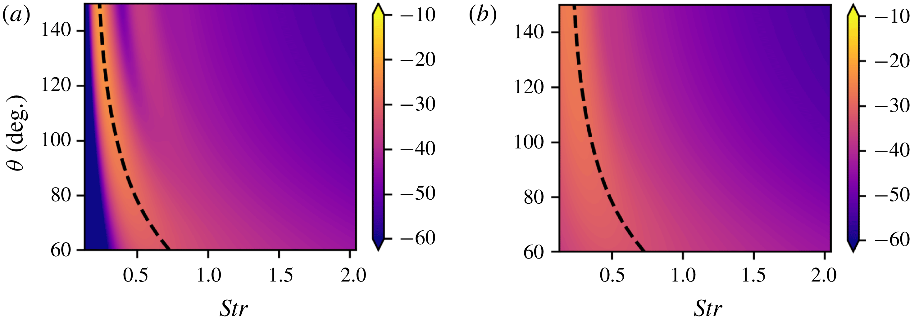
Figure 1. Contours of sound pressure level (arbitrary dB) as a function of frequency (
 $St$
) and directivity (
$St$
) and directivity (
 $\unicode[STIX]{x1D703}$
) for (a) unit coherence and (b) with coherence decay. The jet issues from a converging nozzle (
$\unicode[STIX]{x1D703}$
) for (a) unit coherence and (b) with coherence decay. The jet issues from a converging nozzle (
 $M_{d}=1.0$
) at a nozzle pressure ratio of
$M_{d}=1.0$
) at a nozzle pressure ratio of
 $NPR=3.4$
which corresponds to a fully expanded jet Mach number of
$NPR=3.4$
which corresponds to a fully expanded jet Mach number of
 $M_{j}=1.45$
and an off-design parameter of
$M_{j}=1.45$
and an off-design parameter of
 $\unicode[STIX]{x1D6FD}=1.04$
. The dashed line indicates the peak frequency as predicted by Harper-Bourne & Fisher (Reference Harper-Bourne and Fisher1973).
$\unicode[STIX]{x1D6FD}=1.04$
. The dashed line indicates the peak frequency as predicted by Harper-Bourne & Fisher (Reference Harper-Bourne and Fisher1973).
The first stage of the analysis considers cases involving a single shock-cell mode (
 $n=1$
); the centreline pressure fluctuations in a moderately underexpanded jet are reasonably well represented by a single mode (Tam, Jackson & Seiner Reference Tam, Jackson and Seiner1985; Ray & Lele Reference Ray and Lele2007). Figure 2 shows the directivity for far-field SPL at
$n=1$
); the centreline pressure fluctuations in a moderately underexpanded jet are reasonably well represented by a single mode (Tam, Jackson & Seiner Reference Tam, Jackson and Seiner1985; Ray & Lele Reference Ray and Lele2007). Figure 2 shows the directivity for far-field SPL at
 $St=0.3$
and
$St=0.3$
and
 $St=0.6$
for the same conditions as figure 1 but with only the fundamental shock-cell mode (
$St=0.6$
for the same conditions as figure 1 but with only the fundamental shock-cell mode (
 $n=1$
) included. The Strouhal number is defined as
$n=1$
) included. The Strouhal number is defined as
 $St=fD/U_{j}$
. Models with unit coherence and coherence decay are plotted on the same figure for comparison. At
$St=fD/U_{j}$
. Models with unit coherence and coherence decay are plotted on the same figure for comparison. At
 $St=0.3$
, both models predict the highest amplitude of radiation in the direction slightly upstream of perpendicular, consistent with previous findings. At
$St=0.3$
, both models predict the highest amplitude of radiation in the direction slightly upstream of perpendicular, consistent with previous findings. At
 $St=0.6$
, the BBSAN peaks shift downstream but with a smaller sound amplitude. With all other terms equal, the introduction of coherence decay broadens the radiation lobe, increasing the SPL in the downstream direction (low
$St=0.6$
, the BBSAN peaks shift downstream but with a smaller sound amplitude. With all other terms equal, the introduction of coherence decay broadens the radiation lobe, increasing the SPL in the downstream direction (low
 $\unicode[STIX]{x1D703}$
values). Contrary to the subsonic jet case (Cavalieri et al.
Reference Cavalieri, Jordan, Agarwal and Gervais2011; Baqui et al.
Reference Baqui, Agarwal, Cavalieri and Sinayoko2015, amongst others), however, the introduction of coherence decay reduces the peak amplitude by approximately 2–5 dB. The reason for this behaviour will be further explored in § 4. It is also evident, from the peak frequency trends in figures 1 and 2, that the current wavepacket model agrees with the predictions made by localised phased-array models such as Harper-Bourne & Fisher (Reference Harper-Bourne and Fisher1973).
$\unicode[STIX]{x1D703}$
values). Contrary to the subsonic jet case (Cavalieri et al.
Reference Cavalieri, Jordan, Agarwal and Gervais2011; Baqui et al.
Reference Baqui, Agarwal, Cavalieri and Sinayoko2015, amongst others), however, the introduction of coherence decay reduces the peak amplitude by approximately 2–5 dB. The reason for this behaviour will be further explored in § 4. It is also evident, from the peak frequency trends in figures 1 and 2, that the current wavepacket model agrees with the predictions made by localised phased-array models such as Harper-Bourne & Fisher (Reference Harper-Bourne and Fisher1973).
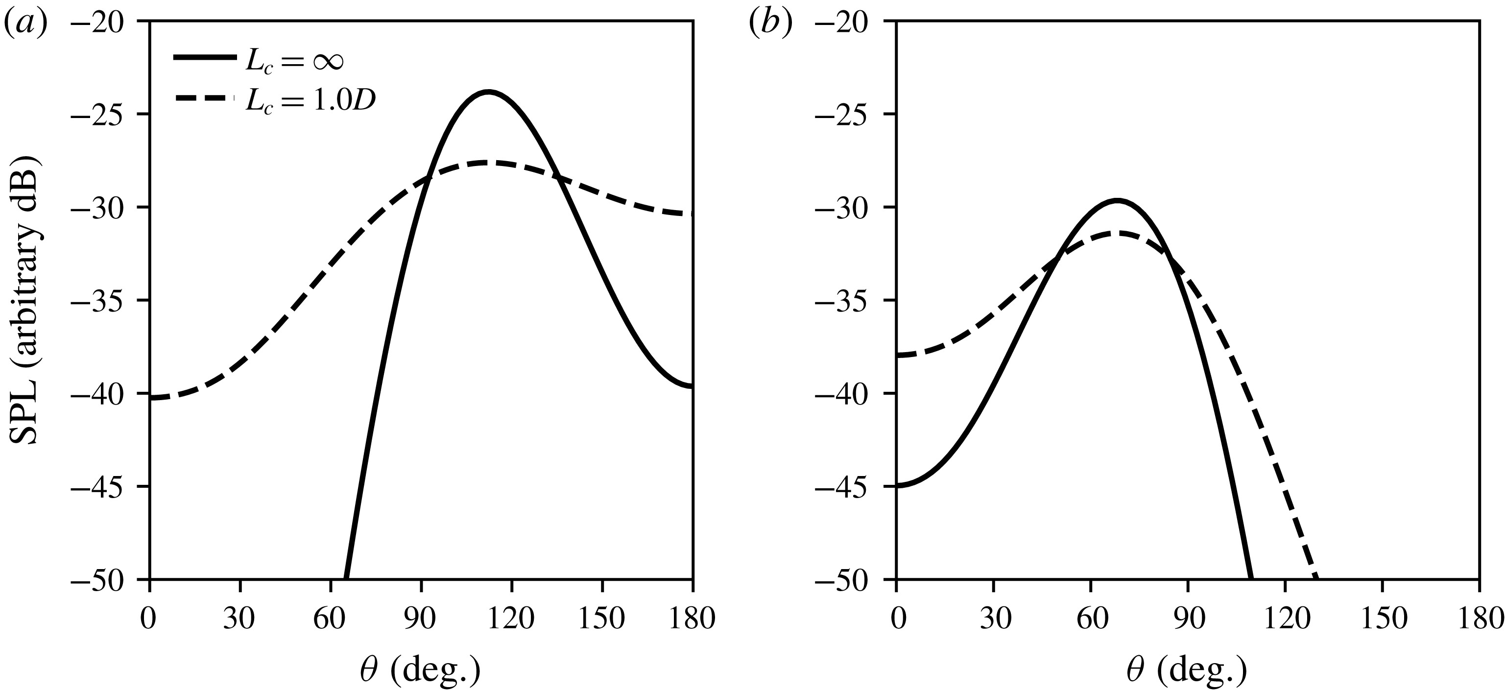
Figure 2. Sound pressure level at a distance of
 $100D$
for a wavepacket frequency of (a)
$100D$
for a wavepacket frequency of (a)
 $St=0.3$
and (b)
$St=0.3$
and (b)
 $St=0.6$
as a function of observation angle
$St=0.6$
as a function of observation angle
 $\unicode[STIX]{x1D703}$
for a wavepacket with
$\unicode[STIX]{x1D703}$
for a wavepacket with
 $k_{h}L=5$
.
$k_{h}L=5$
.
Figure 3 shows a comparison of the noise spectra between the two models and experimental data for an underexpanded jet operating at
 $NPR=3.4$
(Norum & Seiner Reference Norum and Seiner1982). The modelled peak amplitudes are adjusted to match experimental data in order to facilitate comparison of the spectral shape. As can be seen, while there is reasonable agreement between the two models and the measured data in terms of the peak frequency, the overall agreement between the two models and the data is moderate. Both the unit-coherence and coherence-decay models capture the BBSAN peak frequency dependence and the narrowing of the spectral peak with increasing angle. With the inclusion of coherence decay, however, the BBSAN spectral peak width broadens leading to a more favourable agreement for frequencies greater than the peak. Below
$NPR=3.4$
(Norum & Seiner Reference Norum and Seiner1982). The modelled peak amplitudes are adjusted to match experimental data in order to facilitate comparison of the spectral shape. As can be seen, while there is reasonable agreement between the two models and the measured data in terms of the peak frequency, the overall agreement between the two models and the data is moderate. Both the unit-coherence and coherence-decay models capture the BBSAN peak frequency dependence and the narrowing of the spectral peak with increasing angle. With the inclusion of coherence decay, however, the BBSAN spectral peak width broadens leading to a more favourable agreement for frequencies greater than the peak. Below
 $\unicode[STIX]{x1D703}=75^{\circ }$
, both models fail to capture the correct peak frequency. A possible explanation for this disagreement in peak frequency at downstream angles could be due to the choice of the
$\unicode[STIX]{x1D703}=75^{\circ }$
, both models fail to capture the correct peak frequency. A possible explanation for this disagreement in peak frequency at downstream angles could be due to the choice of the
 $u_{c}$
and
$u_{c}$
and
 $L$
modelling variables, as discussed in appendix A, or the dominance of jet mixing noise close to the jet axis.
$L$
modelling variables, as discussed in appendix A, or the dominance of jet mixing noise close to the jet axis.
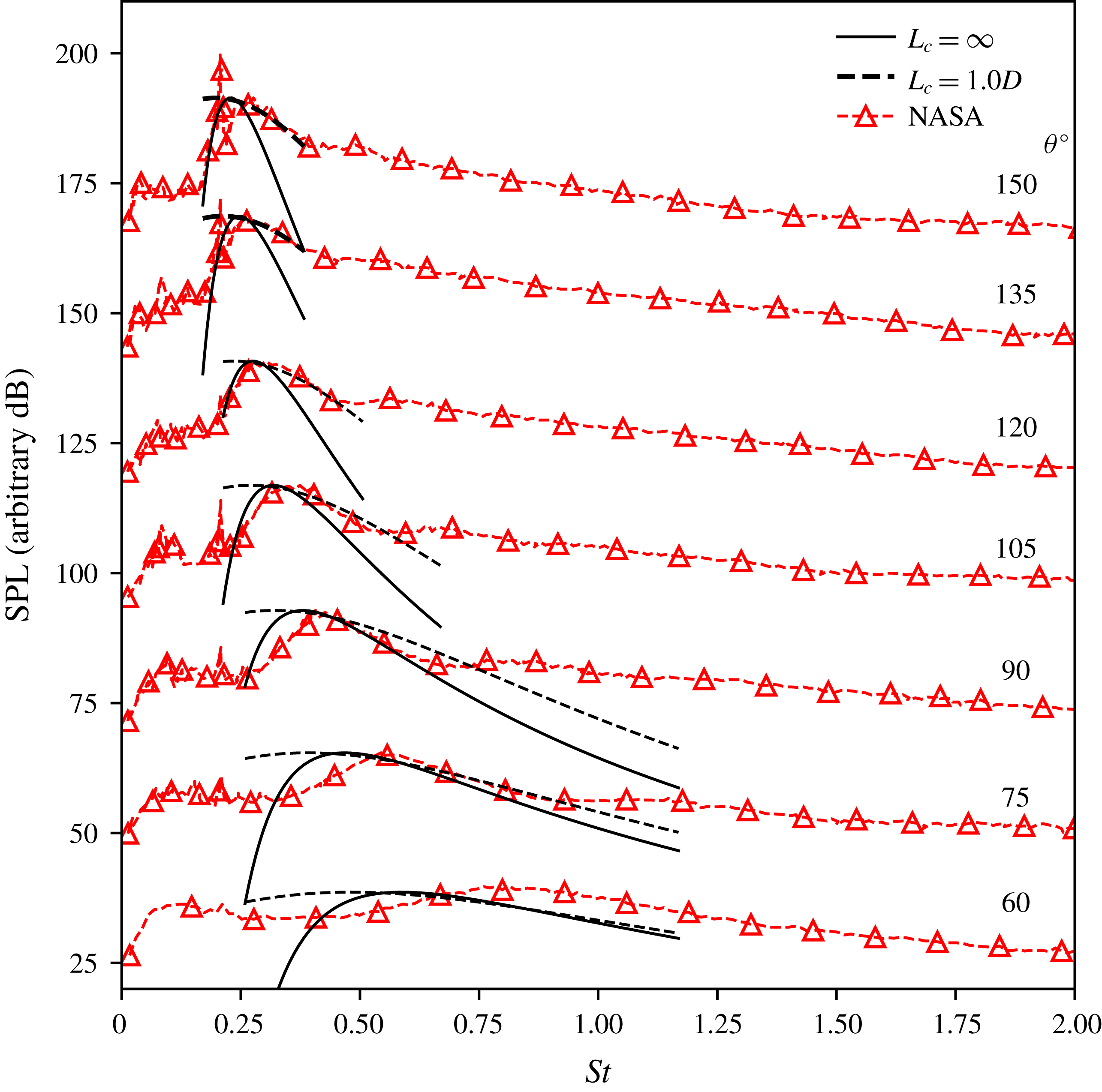
Figure 3. Power spectrum at a distance of
 $100D$
through a range of observation angles between
$100D$
through a range of observation angles between
 $\unicode[STIX]{x1D703}=60^{\circ }$
and
$\unicode[STIX]{x1D703}=60^{\circ }$
and
 $\unicode[STIX]{x1D703}=150^{\circ }$
measured from the downstream jet axis for a wavepacket with
$\unicode[STIX]{x1D703}=150^{\circ }$
measured from the downstream jet axis for a wavepacket with
 $k_{h}L=5$
. Each measurement angle is offset by
$k_{h}L=5$
. Each measurement angle is offset by
 $\unicode[STIX]{x0394}dB=25$
. NASA experimental data from Norum & Seiner (Reference Norum and Seiner1982).
$\unicode[STIX]{x0394}dB=25$
. NASA experimental data from Norum & Seiner (Reference Norum and Seiner1982).
It is evident from figure 3 that the jitter of wavepackets, modelled by coherence decay, broadens the acoustic spectrum. The model suggests, however, that coherence decay does not have a major impact on the sound amplitude. Unlike in subsonic flows, it provides little contribution to the peak SPL. This is also consistent with the results presented by Sinha et al. (Reference Sinha, Rodríguez, Brès and Colonius2014) for isothermal fully expanded supersonic jets, where it was found that the far-field noise spectrum at downstream observation angles is well captured even without considering the jitter of wavepackets. The reason for this is because in supersonic ideally expanded flows, wavepackets propagate downstream with supersonic phase velocities. As a result, noise in the form of Mach wave radiation is generated efficiently (Tam Reference Tam1995) in the downstream direction. On the other hand, in shock-containing flows, the presence of shock cells generates an additional component which travels upstream. The effect of jittering, on both upstream- and downstream-travelling components, is discussed in more detail in § 4.
Using a single shock-cell waveguide mode, both wavepacket models show reasonable agreement with the peak of the measured spectrum. However, they suffer from the same issue discussed by Ray & Lele (Reference Ray and Lele2007) where the high-frequency sound at upstream angles is ‘missing’. In their study, for a
 $M_{j}=1.22$
isothermal jet, the frequency range of interest was restricted to
$M_{j}=1.22$
isothermal jet, the frequency range of interest was restricted to
 $St<1$
due to the assumed breakdown of linear theory at high frequencies. More recently, however, it has been shown by Sasaki et al. (Reference Sasaki, Cavalieri, Jordan, Schmidt, Colonius and Brès2017a
) that linear theory still yields good agreement for frequencies up to
$St<1$
due to the assumed breakdown of linear theory at high frequencies. More recently, however, it has been shown by Sasaki et al. (Reference Sasaki, Cavalieri, Jordan, Schmidt, Colonius and Brès2017a
) that linear theory still yields good agreement for frequencies up to
 $St=4$
. Therefore, we argue here that the drop off in high frequency is not due to the breakdown of linear theory but rather neglecting to include higher-order shock-cell modes. This is further supported by Suzuki’s wavepacket model where a similar underestimation of high-frequency SPL was observed when using an empirical representation of the shock cells. The effect of including higher-order modes is discussed in § 5.
$St=4$
. Therefore, we argue here that the drop off in high frequency is not due to the breakdown of linear theory but rather neglecting to include higher-order shock-cell modes. This is further supported by Suzuki’s wavepacket model where a similar underestimation of high-frequency SPL was observed when using an empirical representation of the shock cells. The effect of including higher-order modes is discussed in § 5.
4 Interpretation of sound-radiation characteristics
4.1 Fourier transform into wavenumber space
In order to explore how coherence affects the source structure and sound-radiation characteristics, the CSD of the models with and without coherence decay are transformed to wavenumber space. This transformation is achieved with the double Fourier transform,
 $$\begin{eqnarray}{\mathcal{F}}(k_{y_{1}},k_{y_{2}})=\frac{1}{(\sqrt{2\unicode[STIX]{x03C0}})^{2}}\int _{-\infty }^{\infty }\int _{-\infty }^{\infty }F(y_{1},y_{2})\text{e}^{\text{i}k_{y_{1}}y_{1}}\text{e}^{\text{i}k_{y_{2}}y_{2}}\,\text{d}y_{1}\,\text{d}y_{2},\end{eqnarray}$$
where
 $F(y_{1},y_{2})$
is the two-point expression of the CSD. If we take coherence as unity for the entire domain by inserting (2.12) into (4.1), the Fourier transform for the perfectly coherent model for a single shock-cell mode is
$F(y_{1},y_{2})$
is the two-point expression of the CSD. If we take coherence as unity for the entire domain by inserting (2.12) into (4.1), the Fourier transform for the perfectly coherent model for a single shock-cell mode is
 $$\begin{eqnarray}\displaystyle {\mathcal{F}}(k_{y_{1}},k_{y_{2}}) & = & \displaystyle \frac{1}{(\sqrt{2\unicode[STIX]{x03C0}})^{2}}\int _{-\infty }^{\infty }\int _{-\infty }^{\infty }A_{n=1}^{2}(\unicode[STIX]{x1D714})\text{e}^{-(y_{1}/L)^{2}}\text{e}^{-(y_{2}/L)^{2}}\{\text{e}^{\text{i}k_{s}y_{1}}+\text{e}^{-\text{i}k_{s}y_{1}}\!\}\nonumber\\ \displaystyle & & \displaystyle \times \,\{\text{e}^{\text{i}k_{s}y_{2}}+\text{e}^{-\text{i}k_{s}y_{2}}\}\{\text{e}^{\text{i}k_{h}(y_{1}-y_{2})}\}\text{e}^{\text{i}k_{y_{1}}y_{1}}\text{e}^{\text{i}k_{y_{2}}y_{2}}\,\text{d}y_{1}\,\text{d}y_{2}.\end{eqnarray}$$
Evaluating the above integral gives
 $$\begin{eqnarray}\displaystyle {\mathcal{F}}(k_{y_{1}},k_{y_{2}}) & = & \displaystyle \frac{A_{n=1}^{2}(\unicode[STIX]{x1D714})}{8}(\text{e}^{-(1/4)(k_{h}-k_{s}+k_{y_{1}})^{2}L^{2}}+\text{e}^{-(1/4)(k_{h}+k_{s}+k_{y_{1}})^{2}L^{2}})\nonumber\\ \displaystyle & & \displaystyle \times (\text{e}^{-(1/4)(k_{h}+k_{s}-k_{y_{2}}\!)^{2}L^{2}}+\text{e}^{-(1/4)(-k_{h}+k_{s}+k_{y_{2}})^{2}L^{2}})L^{2},\end{eqnarray}$$
which is the wavenumber spectrum of the perfectly coherent source CSD. Likewise, by inserting (2.15) into (4.1) and evaluating the resulting integral, the Fourier-transformed CSD of the coherence decay model can also be obtained (the solution is presented in appendix B). Equation (4.3) is obtained from (B 1) by taking the limit
 $L_{c}\rightarrow \infty$
.
$L_{c}\rightarrow \infty$
.
Both source CSD models in physical space are shown in figure 4(a,b). In this model problem, the jet nozzle is not present and the sources are simply centred at the origin and extended in both positive and negative directions along the jet axis. The peaks in the contour map are similar to the freckled appearance seen in the two-point pressure correlations obtained by Suzuki (Reference Suzuki2016). As noted by Suzuki, the spacing between the peaks on the diagonal approximately correspond to the shock-cell spacings. The off-diagonal peaks correspond to the wavepacket interacting with adjacent shock cells. The introduction of coherence decay concentrates the sources in space; along the axis
 $y_{1}=y_{2}$
. This behaviour is also seen in the non-shock-containing case, as found by Cavalieri & Agarwal (Reference Cavalieri and Agarwal2014).
$y_{1}=y_{2}$
. This behaviour is also seen in the non-shock-containing case, as found by Cavalieri & Agarwal (Reference Cavalieri and Agarwal2014).

Figure 4. The real part of the CSD of the unit coherence (a) and with statistical decay (b) models for
 $L_{c}=1.0D$
. The diagonal line represents
$L_{c}=1.0D$
. The diagonal line represents
 $y_{1}=y_{2}$
. The corresponding Fourier-transformed CSD in wavenumber space with the unit-coherence (c) and statistical decay (d) models. Diagonal line corresponds to
$y_{1}=y_{2}$
. The corresponding Fourier-transformed CSD in wavenumber space with the unit-coherence (c) and statistical decay (d) models. Diagonal line corresponds to
 $k_{y1}=-k_{y2}$
. The square represents the acoustic matching criterion
$k_{y1}=-k_{y2}$
. The square represents the acoustic matching criterion
 $|k|/k_{h}=0.6M_{j}$
. The amplitudes of both models have been normalised to highlight the effect of coherence decay. The wavepacket frequency is
$|k|/k_{h}=0.6M_{j}$
. The amplitudes of both models have been normalised to highlight the effect of coherence decay. The wavepacket frequency is
 $St=0.4$
for a jet operating at
$St=0.4$
for a jet operating at
 $\unicode[STIX]{x1D6FD}=1.04$
.
$\unicode[STIX]{x1D6FD}=1.04$
.
A comparison of the models’ Fourier-transformed CSDs as given by (4.3) and (B 1) is shown in figure 4(c,d) respectively. The contour scale is logarithmic and both axes are normalised by the hydrodynamic wavenumber of the wavepacket
 $k_{h}$
. The source term in both cases produces four distinct lobes. The existence and ramifications of these are discussed in detail in § 4.2. The introduction of coherence decay stretches the lobes parallel to the
$k_{h}$
. The source term in both cases produces four distinct lobes. The existence and ramifications of these are discussed in detail in § 4.2. The introduction of coherence decay stretches the lobes parallel to the
 $k_{y1}=-k_{y2}$
axis. This is consistent with what has been observed in subsonic jets (Cavalieri & Agarwal Reference Cavalieri and Agarwal2014; Jaunet et al.
Reference Jaunet, Jordan and Cavalieri2017).
$k_{y1}=-k_{y2}$
axis. This is consistent with what has been observed in subsonic jets (Cavalieri & Agarwal Reference Cavalieri and Agarwal2014; Jaunet et al.
Reference Jaunet, Jordan and Cavalieri2017).
As noted by Crighton (Reference Crighton1975), only certain spectral components of the source term corresponding to supersonic phase speeds can contribute to far-field noise. In order to isolate only the radiating wavenumbers of the source term, the following conditions need to be met
 $$\begin{eqnarray}\displaystyle & \displaystyle \frac{|k_{y1}|}{k_{h}}\leqslant M_{c} & \displaystyle\end{eqnarray}$$
 $$\begin{eqnarray}\displaystyle & \displaystyle \frac{|k_{y2}|}{k_{h}}\leqslant M_{c}, & \displaystyle\end{eqnarray}$$
 $M_{c}=\unicode[STIX]{x1D714}/(k_{h}c_{0})$
is the convective Mach number. These conditions in wavenumber space are represented by the squares in figure 4(c,d). Source energy that lies outside the square does not contribute to the far-field sound. Unlike the subsonic jet case, where the unit-coherence source lies completely outside the radiation square, the supersonic shock-containing case already has a source lobe satisfying the radiation criterion. This is similar to what is observed in ideally expanded supersonic jets (Cavalieri & Agarwal Reference Cavalieri and Agarwal2014; Sinha et al.
Reference Sinha, Rodríguez, Brès and Colonius2014). The other three lobes are silent as they lie outside the radiation square.
$M_{c}=\unicode[STIX]{x1D714}/(k_{h}c_{0})$
is the convective Mach number. These conditions in wavenumber space are represented by the squares in figure 4(c,d). Source energy that lies outside the square does not contribute to the far-field sound. Unlike the subsonic jet case, where the unit-coherence source lies completely outside the radiation square, the supersonic shock-containing case already has a source lobe satisfying the radiation criterion. This is similar to what is observed in ideally expanded supersonic jets (Cavalieri & Agarwal Reference Cavalieri and Agarwal2014; Sinha et al.
Reference Sinha, Rodríguez, Brès and Colonius2014). The other three lobes are silent as they lie outside the radiation square.When coherence decay is introduced we see that the stretching of the radiation lobe actually removes a small portion of the source energy from the radiating region. Unlike the subsonic case, where jittering of the wavepacket causes the source energy to be stretched into the radiation square, coherence decay removes energy in the BBSAN case. This explains why the introduction of coherence decay decreases the peak SPL compared to the unit-coherence case as seen in figure 2.
The Fourier transform contour plots can also be used to explain the directivity behaviour observed in figure 2. For a given value of
 $\unicode[STIX]{x1D703}$
, the Fourier-transformed wavenumbers
$\unicode[STIX]{x1D703}$
, the Fourier-transformed wavenumbers
 $k_{y_{1}}$
and
$k_{y_{1}}$
and
 $k_{y_{2}}$
are given by
$k_{y_{2}}$
are given by
 $$\begin{eqnarray}\displaystyle \left(\frac{k_{y_{1}}}{k_{h}},\frac{k_{y_{2}}}{k_{h}}\right)=(-M_{c}\cos \unicode[STIX]{x1D703},M_{c}\cos \unicode[STIX]{x1D703}). & & \displaystyle\end{eqnarray}$$
Therefore, for
 $\unicode[STIX]{x1D703}$
values corresponding to the perpendicular direction, the relevant part of the Fourier transform is close to the origin. Moving away from the origin along this axis will correspond to angles upstream and downstream of the jet axis respectively. Hence, the stretching of the source lobe along the
$\unicode[STIX]{x1D703}$
values corresponding to the perpendicular direction, the relevant part of the Fourier transform is close to the origin. Moving away from the origin along this axis will correspond to angles upstream and downstream of the jet axis respectively. Hence, the stretching of the source lobe along the
 $k_{y_{1}}=-k_{y_{2}}$
axis also broadens the directivity of the jet as depicted in figure 2. This broadening is due to the source energy being stretched in both directions from the origin within the radiation square. To summarise, coherence decay is not a sound amplifier as found in the subsonic case but rather broadens the directivity of BBSAN. This broadening will be seen to be even more important when we consider higher-order shock-cell modes in § 5.
$k_{y_{1}}=-k_{y_{2}}$
axis also broadens the directivity of the jet as depicted in figure 2. This broadening is due to the source energy being stretched in both directions from the origin within the radiation square. To summarise, coherence decay is not a sound amplifier as found in the subsonic case but rather broadens the directivity of BBSAN. This broadening will be seen to be even more important when we consider higher-order shock-cell modes in § 5.
4.2 Nonlinear interaction terms
By transforming the CSD from physical space to wavenumber space, it has been demonstrated that not all wavelengths of the line-source model are responsible for sound generation. The source lobes seen in wavenumber space are due to the nonlinear interactions present in this BBSAN model. As previously mentioned, only source components corresponding to supersonic phase speeds relative to the ambient speed of sound can be effective BBSAN noise generators. In order to test whether the acoustically matched source component is supersonic, we aim to identify the phase speeds of the four source lobes in wavenumber space.
Recall that the kinematic model comprises the multiplicative combination of the wavepacket and the shock-cell structure as described in (2.4). Using the unit-coherence case for simplicity, after expanding the shock-cell components, the source term in (2.12) can be written as
 $$\begin{eqnarray}\displaystyle S(y_{1},\unicode[STIX]{x1D714})S^{\ast }(y_{2},\unicode[STIX]{x1D714})=\mathop{\sum }_{n}\{\text{e}^{\text{i}k_{s}(y_{1}+y_{2})}+\text{e}^{\text{i}k_{s}(y_{1}-y_{2})}+\text{e}^{\text{i}k_{s}(-y_{1}+y_{2})}+\text{e}^{\text{i}k_{s}(-y_{1}-y_{2})}\}\{\text{e}^{\text{i}k_{h}(y_{1}-y_{2})}\},\quad & & \displaystyle\end{eqnarray}$$
where we have ignored the amplitude and wavepacket envelope terms for this analysis. Expanding again we obtain four terms defined as
 $$\begin{eqnarray}S(y_{1},\unicode[STIX]{x1D714})S^{\ast }(y_{2},\unicode[STIX]{x1D714})=A_{1,2}^{+}+A_{1,2}^{-}+B_{1,2}^{+}+B_{1,2}^{-},\end{eqnarray}$$
where the terms are shown to be
 $$\begin{eqnarray}\displaystyle & \displaystyle A_{1,2}^{+}=\text{e}^{\text{i}(y_{1}-y_{2})(k_{h}+k_{s})}, & \displaystyle\end{eqnarray}$$
 $$\begin{eqnarray}\displaystyle & \displaystyle A_{1,2}^{-}=\text{e}^{\text{i}(y_{1}-y_{2})(k_{h}-k_{s})}, & \displaystyle\end{eqnarray}$$
 $$\begin{eqnarray}\displaystyle & \displaystyle B_{1,2}^{+}=\text{e}^{\text{i}y_{1}(k_{s}+k_{h})+\text{i}y_{2}(k_{s}-k_{h})}, & \displaystyle\end{eqnarray}$$
 $$\begin{eqnarray}\displaystyle & \displaystyle B_{1,2}^{-}=\text{e}^{\text{i}y_{1}(-k_{s}+k_{h})+\text{i}y_{2}(-k_{s}-k_{h})}. & \displaystyle\end{eqnarray}$$
By grouping the terms in this manner, we see that the
 $A_{1,2}^{+}$
and
$A_{1,2}^{+}$
and
 $A_{1,2}^{-}$
terms, which are respectively the sum and difference nonlinear wave interactions, have phase velocities
$A_{1,2}^{-}$
terms, which are respectively the sum and difference nonlinear wave interactions, have phase velocities
 $$\begin{eqnarray}\displaystyle & \displaystyle v^{+}=\frac{\unicode[STIX]{x1D714}}{k_{h}+k_{s}}, & \displaystyle\end{eqnarray}$$
 $$\begin{eqnarray}\displaystyle & \displaystyle v^{-}=\frac{\unicode[STIX]{x1D714}}{k_{h}-k_{s}}. & \displaystyle\end{eqnarray}$$
Since
 $\unicode[STIX]{x1D714}/(k_{h})>\unicode[STIX]{x1D714}/(k_{h}+k_{s})$
, the
$\unicode[STIX]{x1D714}/(k_{h})>\unicode[STIX]{x1D714}/(k_{h}+k_{s})$
, the
 $A_{1,2}^{+}$
component travels slower than the ambient speed of sound and is not acoustically matched. It corresponds to the top left lobe in figure 4(c,d) along the diagonal. Conversely, the term
$A_{1,2}^{+}$
component travels slower than the ambient speed of sound and is not acoustically matched. It corresponds to the top left lobe in figure 4(c,d) along the diagonal. Conversely, the term
 $A_{1,2}^{-}$
is capable of either subsonic or supersonic phase speeds and is represented by the bottom right lobe in figure 4(c,d). This explains why only the
$A_{1,2}^{-}$
is capable of either subsonic or supersonic phase speeds and is represented by the bottom right lobe in figure 4(c,d). This explains why only the
 $A_{1,2}^{-}$
component of the total source term is capable of generating far-field noise and is consistent with previous findings (Tam & Tanna Reference Tam and Tanna1982).
$A_{1,2}^{-}$
component of the total source term is capable of generating far-field noise and is consistent with previous findings (Tam & Tanna Reference Tam and Tanna1982).
The terms
 $B_{1,2}^{+}$
and
$B_{1,2}^{+}$
and
 $B_{1,2}^{-}$
, on the other hand, involve combined effects of the sum and difference interaction and are a complex conjugate pair. These terms, however, lie off the
$B_{1,2}^{-}$
, on the other hand, involve combined effects of the sum and difference interaction and are a complex conjugate pair. These terms, however, lie off the
 $k_{y1}=-k_{y2}$
axis and outside the radiation square and therefore do not contribute to the far-field sound. A similar depiction of these off-diagonal lobes are observed in the Fourier-transformed CSD maps of Baqui et al. (Reference Baqui, Agarwal, Cavalieri and Sinayoko2015) and nonlinear wavenumber interactions in low Reynolds number subsonic jets as discussed by Sandham, Morfey & Hu (Reference Sandham, Morfey and Hu2006).
$k_{y1}=-k_{y2}$
axis and outside the radiation square and therefore do not contribute to the far-field sound. A similar depiction of these off-diagonal lobes are observed in the Fourier-transformed CSD maps of Baqui et al. (Reference Baqui, Agarwal, Cavalieri and Sinayoko2015) and nonlinear wavenumber interactions in low Reynolds number subsonic jets as discussed by Sandham, Morfey & Hu (Reference Sandham, Morfey and Hu2006).
5 Coherence decay and higher-order shock-cell modes
We now focus on the more general model where higher-order shock-cell modes are included. It has been demonstrated that these additional shock-cell modes do make significant contributions to high frequency sound in the upstream directions (Tam et al. Reference Tam, Jackson and Seiner1985; Ray & Lele Reference Ray and Lele2007). We here test the effect of coherence decay when these higher-order shock-cell modes are included.
Tam et al. (Reference Tam, Jackson and Seiner1985) have argued that it should only be necessary to include the first four shock-cell modes and any higher modes are unnecessary to describe the shock-cell structure. Ray & Lele (Reference Ray and Lele2007), on the other hand, justified the use of only the fundamental shock-cell mode as source activity associated with higher-order modes lie outside the range of radiating wavenumbers. This is true when coherence decay is not accounted for.
The sensitivity of the acoustic spectrum to the addition of higher-order shock-cell modes was investigated for the current source model. It was found that the far-field spectrum and source structure did not change significantly beyond the first ten modes. Hence only the first ten shock-cell modes, as defined by (2.6), were used for this study.
By including higher-order modes, as shown by figure 5, an improvement in spectral shape is observed for all observation angles. Higher waveguide modes are required to describe the acoustic spectra for frequencies greater than the broadband peak, consistent with Tam et al. (Reference Tam, Jackson and Seiner1985). While there are still discrepancies for the downstream angle at
 $\unicode[STIX]{x1D703}=60^{\circ }$
, both models predict the peak frequency with reasonable accuracy, although the case with coherence decay slightly underpredicts the peak frequency compared to the data. The spectral peak shape predicted when coherence decay is included is more accurate than the case with perfect coherence. For the perfectly coherent wavepacket, oscillations start to occur at higher Strouhal numbers resulting in ‘narrow-banded’ secondary peaks. This deficiency of the perfectly coherent model at higher frequencies for upstream angles agrees with Ray & Lele (Reference Ray and Lele2007) where it was found that the linear model (unit coherence by construction) becomes ‘increasingly suspect at higher frequencies’.
$\unicode[STIX]{x1D703}=60^{\circ }$
, both models predict the peak frequency with reasonable accuracy, although the case with coherence decay slightly underpredicts the peak frequency compared to the data. The spectral peak shape predicted when coherence decay is included is more accurate than the case with perfect coherence. For the perfectly coherent wavepacket, oscillations start to occur at higher Strouhal numbers resulting in ‘narrow-banded’ secondary peaks. This deficiency of the perfectly coherent model at higher frequencies for upstream angles agrees with Ray & Lele (Reference Ray and Lele2007) where it was found that the linear model (unit coherence by construction) becomes ‘increasingly suspect at higher frequencies’.
Conversely, the two-point model with coherence decay ‘smooths’ out these narrow-banded peaks. This observation is consistent with Ray & Lele’s (Reference Ray and Lele2007) assertion that nonlinear effects can rectify these artificial peaks introduced from the instability wave interacting with the higher-order shock-cell modes. This finding is also consistent with the effect of coherence decay when using localised acoustic sources (Lele Reference Lele2005). We turn to the Fourier-transformed CSD maps to gain an insight into this behaviour.
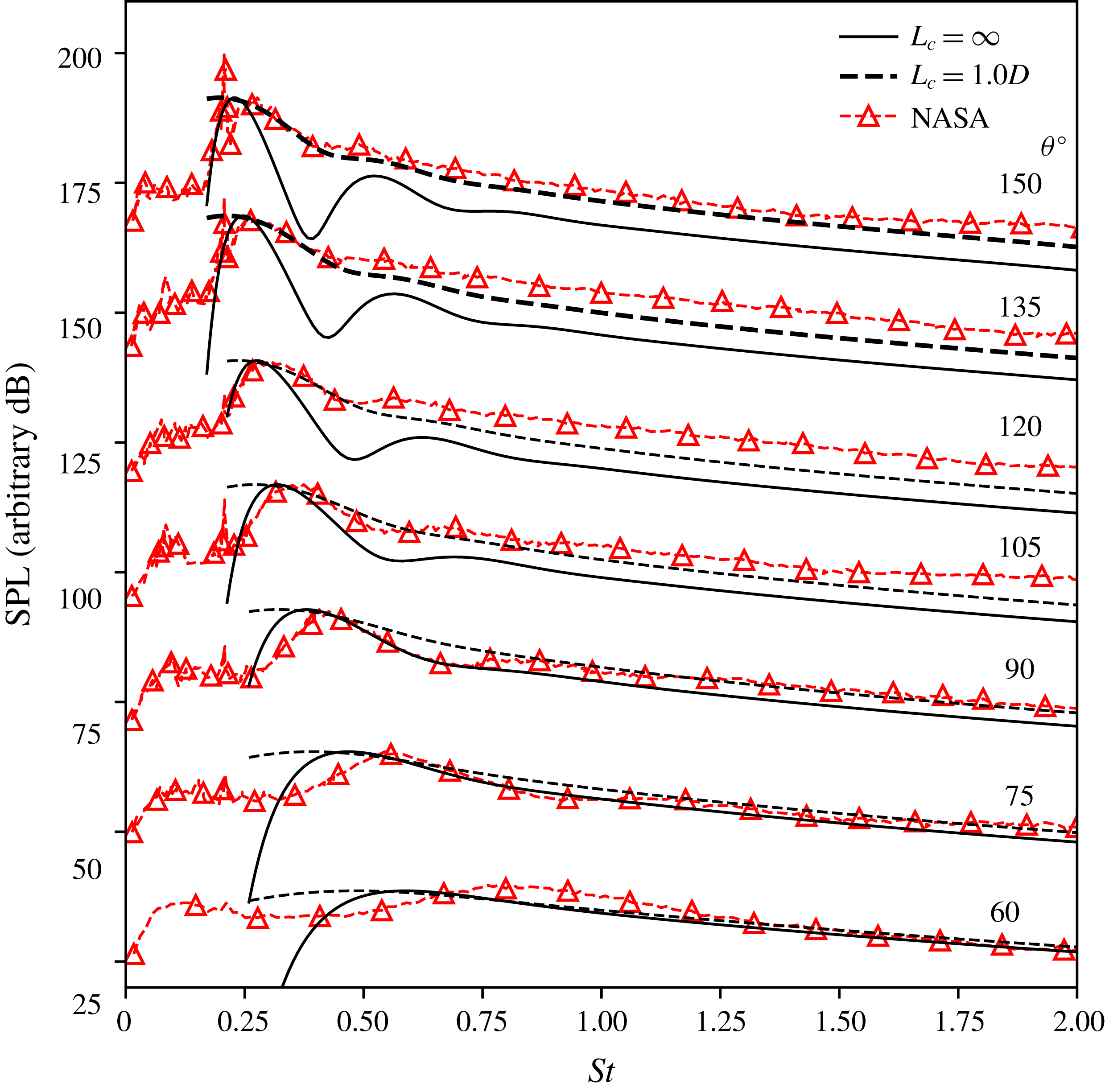
Figure 5. Power spectrum at a distance of
 $100D$
through a range of observation angles between
$100D$
through a range of observation angles between
 $\unicode[STIX]{x1D703}=60^{\circ }$
and
$\unicode[STIX]{x1D703}=60^{\circ }$
and
 $\unicode[STIX]{x1D703}=150^{\circ }$
measured from the downstream jet axis for a wavepacket with
$\unicode[STIX]{x1D703}=150^{\circ }$
measured from the downstream jet axis for a wavepacket with
 $k_{h}L=5$
for multiple shock-cell waveguide modes. Each measurement angle is offset by 25 dB. NASA experimental data from Norum & Seiner (Reference Norum and Seiner1982).
$k_{h}L=5$
for multiple shock-cell waveguide modes. Each measurement angle is offset by 25 dB. NASA experimental data from Norum & Seiner (Reference Norum and Seiner1982).
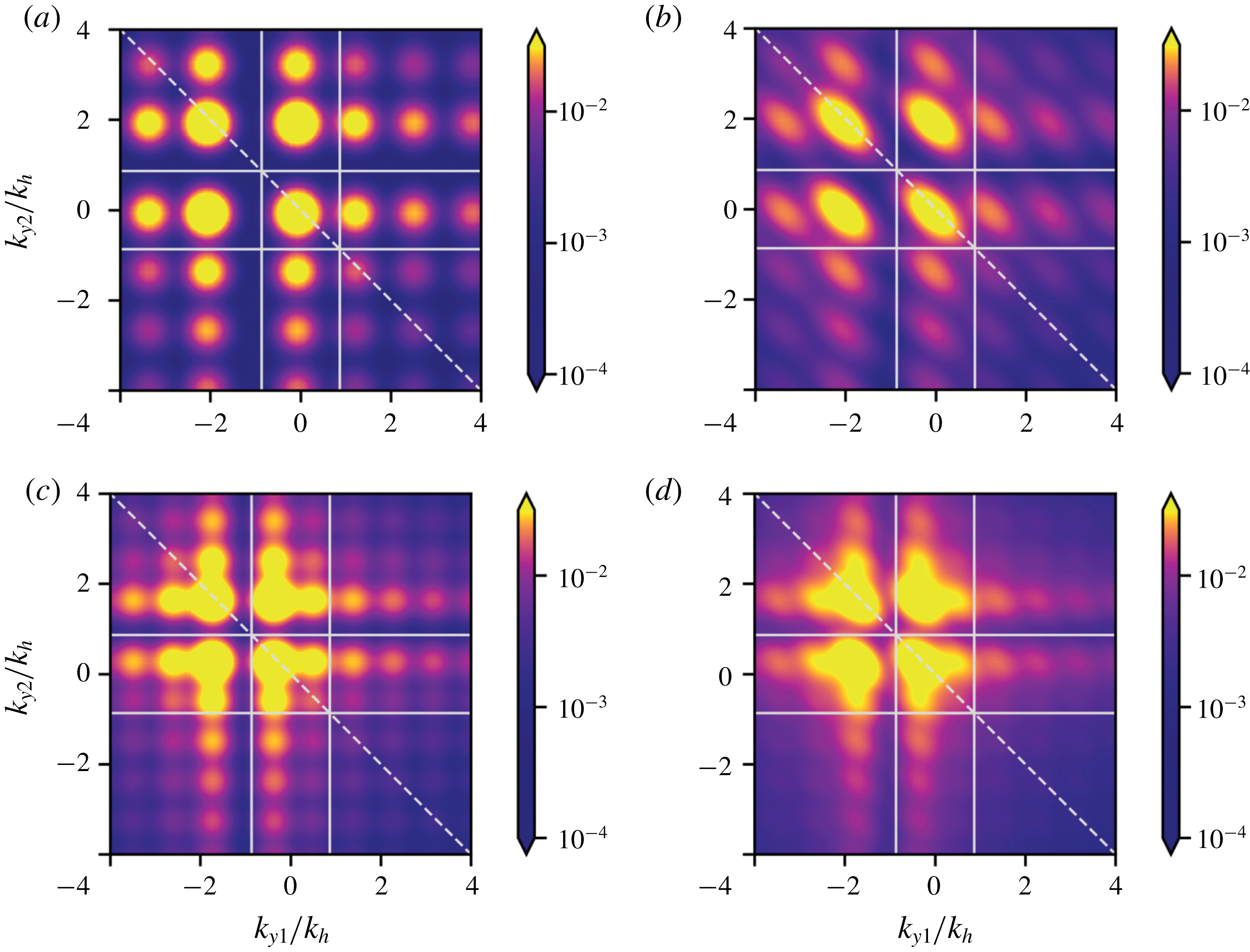
Figure 6. The corresponding Fourier-transformed CSD in wavenumber space for
 $St=0.4$
and
$St=0.4$
and
 $St=0.6$
. (a,c) Correspond to the unit-coherence model while (b,d) are for the two-point model with a coherence-decay length
$St=0.6$
. (a,c) Correspond to the unit-coherence model while (b,d) are for the two-point model with a coherence-decay length
 $L_{c}=1.0D$
. Diagonal line corresponds to
$L_{c}=1.0D$
. Diagonal line corresponds to
 $k_{y_{1}}=-k_{y_{2}}$
. The square represents the acoustic matching criterion
$k_{y_{1}}=-k_{y_{2}}$
. The square represents the acoustic matching criterion
 $|k|/k_{h}=0.6M_{j}$
. The amplitude of both models has been normalised to highlight the effect of coherence decay. The jet is operating at
$|k|/k_{h}=0.6M_{j}$
. The amplitude of both models has been normalised to highlight the effect of coherence decay. The jet is operating at
 $\unicode[STIX]{x1D6FD}=1.04$
.
$\unicode[STIX]{x1D6FD}=1.04$
.
The Fourier-transformed CSD maps are computed for two frequencies,
 $St=0.4$
(figure 6
a,b) and
$St=0.4$
(figure 6
a,b) and
 $St=0.6$
(figure 6
c,d) where we have now included the first ten shock-cell waveguide modes. Compared to the previous single-mode (
$St=0.6$
(figure 6
c,d) where we have now included the first ten shock-cell waveguide modes. Compared to the previous single-mode (
 $n=1$
) case, additional lobes are now visible throughout the wavenumber domain. The additional source-energy lobes are due to the wavepackets interacting with the higher-order Fourier shock-cell modes.
$n=1$
) case, additional lobes are now visible throughout the wavenumber domain. The additional source-energy lobes are due to the wavepackets interacting with the higher-order Fourier shock-cell modes.
For the unit-coherence case (figure 6
a,c), the far-field sound radiation is still dominated by the wavepacket interaction with the
 $n=1$
waveguide mode. For
$n=1$
waveguide mode. For
 $St=0.4$
, interaction with the second mode does not contribute to the far-field radiation as the source energy from this interaction lies outside the radiation square. This is what was observed by Ray & Lele (Reference Ray and Lele2007) and it was the reason modes higher than the fundamental were not considered in their study. At a higher frequency (
$St=0.4$
, interaction with the second mode does not contribute to the far-field radiation as the source energy from this interaction lies outside the radiation square. This is what was observed by Ray & Lele (Reference Ray and Lele2007) and it was the reason modes higher than the fundamental were not considered in their study. At a higher frequency (
 $St=0.6$
), however, the Fourier lobes become more compact and the
$St=0.6$
), however, the Fourier lobes become more compact and the
 $n=2$
modes migrate into the radiation square as seen in figure 6(c). This is consistent with the behaviour seen in the far-field acoustic spectrum of figures 3 and 5. For frequencies below the broadband peak, we do not see an increase in SPL when higher-order shock modes are added.
$n=2$
modes migrate into the radiation square as seen in figure 6(c). This is consistent with the behaviour seen in the far-field acoustic spectrum of figures 3 and 5. For frequencies below the broadband peak, we do not see an increase in SPL when higher-order shock modes are added.
For the model where coherence decay is taken into account (figure 6
b,d), we observe once again a stretching of the source lobes parallel to the
 $k_{y_{1}}=-k_{y_{2}}$
line. The stretching causes the fundamental (
$k_{y_{1}}=-k_{y_{2}}$
line. The stretching causes the fundamental (
 $n=1$
) mode to merge with the second mode and spreads the source energy within the radiating square. In contrast to the unit-coherence case, the
$n=1$
) mode to merge with the second mode and spreads the source energy within the radiating square. In contrast to the unit-coherence case, the
 $n=2$
shock-cell mode is now also responsible for far-field sound production. This means that coherence decay, which accounts for stochastic effects, can rectify the ‘missing sound’ at higher frequencies in the upstream direction seen in figure 3. It is clear, when compared to the perfectly coherent wavepacket, coherence decay ‘spreads and smooths’ the source energy in wavenumber space. This leads to a more uniform far-field spectrum for all observation angles and, indeed, a smoother directivity also results. This levelling effect in both directivity and frequency is evident when comparing the SPL contour plots in figure 1(a,b). Nevertheless, the overprediction in SPL for frequencies below the spectral peak is still present for all observation angles. The overprediction at low frequencies is most likely a result of the ad hoc constant coherence length assumption.
$n=2$
shock-cell mode is now also responsible for far-field sound production. This means that coherence decay, which accounts for stochastic effects, can rectify the ‘missing sound’ at higher frequencies in the upstream direction seen in figure 3. It is clear, when compared to the perfectly coherent wavepacket, coherence decay ‘spreads and smooths’ the source energy in wavenumber space. This leads to a more uniform far-field spectrum for all observation angles and, indeed, a smoother directivity also results. This levelling effect in both directivity and frequency is evident when comparing the SPL contour plots in figure 1(a,b). Nevertheless, the overprediction in SPL for frequencies below the spectral peak is still present for all observation angles. The overprediction at low frequencies is most likely a result of the ad hoc constant coherence length assumption.
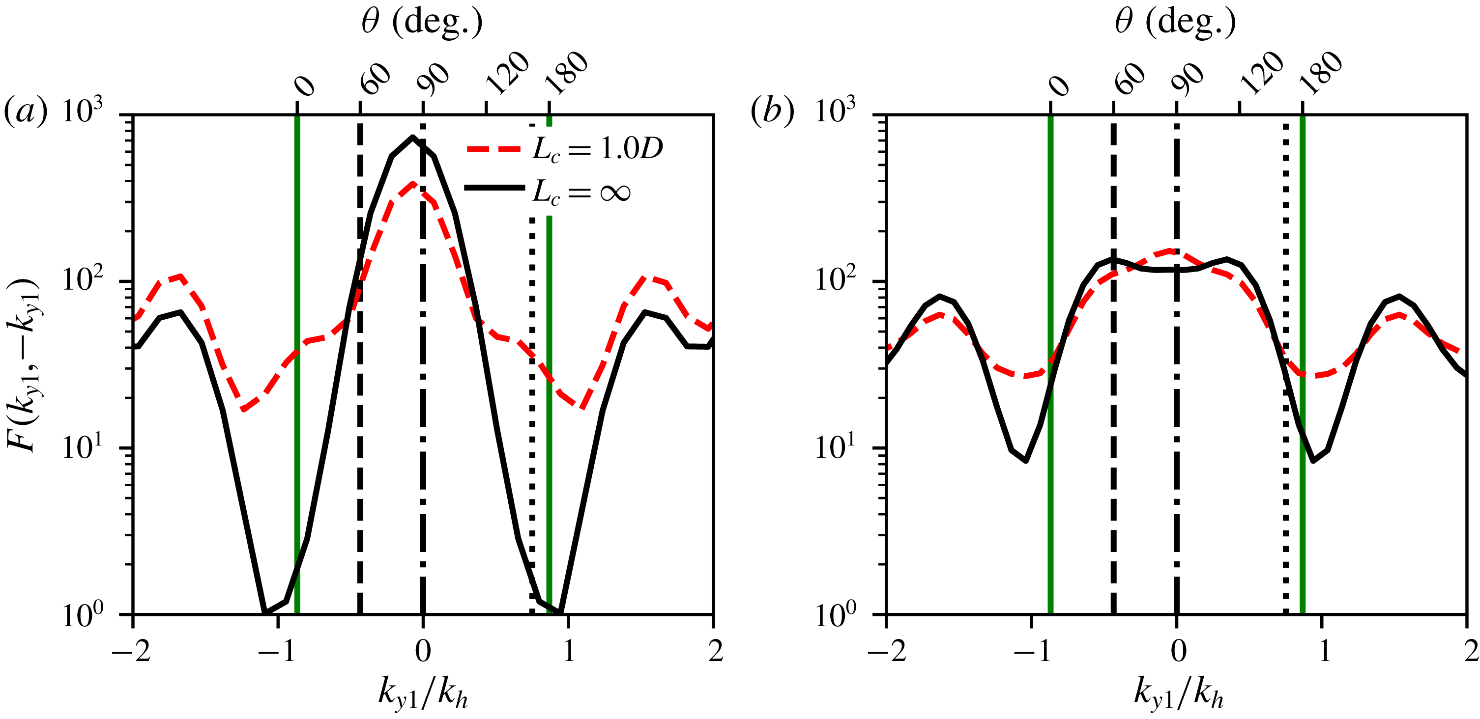
Figure 7. Fourier transform of CSD for (a)
 $St=0.4$
and (b)
$St=0.4$
and (b)
 $St=0.6$
extracted along the line
$St=0.6$
extracted along the line
 $k_{y_{1}}=-k_{y_{2}}$
. The vertical lines represent different observation angles; dashed line
$k_{y_{1}}=-k_{y_{2}}$
. The vertical lines represent different observation angles; dashed line
 $=60^{\circ }$
, dash-dotted line
$=60^{\circ }$
, dash-dotted line
 $=90^{\circ }$
and dotted line
$=90^{\circ }$
and dotted line
 $=150^{\circ }$
. Solid (green) vertical lines represent the acoustic matching criterion.
$=150^{\circ }$
. Solid (green) vertical lines represent the acoustic matching criterion.
Suzuki (Reference Suzuki2016) has also incorporated the effect of coherence decay of wavepackets into his model. However, the empirical treatment of the shock cells as Gaussian humps does not allow the previously discussed effects of coherence decay to be observed. Similar to Ray & Lele (Reference Ray and Lele2007), the loss of high-frequency sound can be attributed to the lack of representation of the higher-order shock-cell modes. The predictions from both Suzuki’s and Ray & Lele’s models are closer to those of figure 3 and hence lack the same agreement to experimental data as other phased-array models such as Harper-Bourne & Fisher (Reference Harper-Bourne and Fisher1973) and Morris & Miller (Reference Morris and Miller2010).
To show the impact of coherence decay on noise directivity more clearly, the Fourier-transformed points along the
 $k_{y_{1}}=-k_{y_{2}}$
line are extracted and shown as dashed lines in figure 7(a,b). Vertical lines corresponding to different radiation directions as specified by (4.5) are also shown for reference. For frequencies slightly greater than the BBSAN peak (
$k_{y_{1}}=-k_{y_{2}}$
line are extracted and shown as dashed lines in figure 7(a,b). Vertical lines corresponding to different radiation directions as specified by (4.5) are also shown for reference. For frequencies slightly greater than the BBSAN peak (
 $St=0.4$
), coherence decay amplifies the radiated sound in the upstream direction and smooths out the artificial peaks seen in the perfectly coherent case. On the other hand, for higher frequencies (
$St=0.4$
), coherence decay amplifies the radiated sound in the upstream direction and smooths out the artificial peaks seen in the perfectly coherent case. On the other hand, for higher frequencies (
 $St=0.6$
), the second shock-cell mode is now also contributing to the far-field sound and the effect of coherence decay is minimal. Comparing this to linear instability model results from Ray & Lele (Reference Ray and Lele2007), the impact of coherence decay on higher frequencies is now apparent.
$St=0.6$
), the second shock-cell mode is now also contributing to the far-field sound and the effect of coherence decay is minimal. Comparing this to linear instability model results from Ray & Lele (Reference Ray and Lele2007), the impact of coherence decay on higher frequencies is now apparent.
Due to the ad hoc nature of fixing the modelling parameters to constant values, it is important to establish that changing the combinations and values does not lead to different conclusions. This is done in appendix A. We find, amongst other effects, that the suppression of the narrow-banded peaks cannot be accounted for by the tuning of
 $u_{c}$
,
$u_{c}$
,
 $A(\unicode[STIX]{x1D714})$
and
$A(\unicode[STIX]{x1D714})$
and
 $L$
within values realistic for supersonic underexpanded jets. We conclude that the inclusion of coherence decay, in the wavepacket framework, is thus imperative. In order to improve predictions at higher frequencies for BBSAN, not only do we need high-order shock modes but also the stochastic forcing term, which in the kinematic model is represented by coherence decay.
$L$
within values realistic for supersonic underexpanded jets. We conclude that the inclusion of coherence decay, in the wavepacket framework, is thus imperative. In order to improve predictions at higher frequencies for BBSAN, not only do we need high-order shock modes but also the stochastic forcing term, which in the kinematic model is represented by coherence decay.
The importance of coherence in BBSSAN source modelling has been well recognised since Harper-Bourne & Fisher’s original model. Using the present BBSAN wavepacket model, however, we suggest that the overall two-point coherence contains much non-acoustically efficient information and that only the coherence decay of the low-order azimuthal modes (wavepackets) is critical in predicting far-field sound. This further suggests a mechanistic explanation for coherence decay in these systems: the coherence decay across sound sources of existing BBSAN models results from the jittering of wavepackets (Williams & Kempton Reference Williams and Kempton1978; Cavalieri et al. Reference Cavalieri, Jordan, Agarwal and Gervais2011).
6 Conclusions and perspectives
Motivated by the pioneering work of Tam (Reference Tam1987), the BBSAN models proposed by Ray & Lele (Reference Ray and Lele2007) and Suzuki (Reference Suzuki2016) indicate the suitability of using wavepackets for this component of jet noise. While successful in predicting many of the known features, the simplified models could not accurately capture the high-frequency sound produced at upstream angles. This is in contrast to the largely accurate predictions made by wavepacket models for supersonic ideally expanded flows (Sinha et al. Reference Sinha, Rodríguez, Brès and Colonius2014). Wavepacket modelling of subsonic jets suggest that coherence decay of the large-scale structures is critical in those flows. Previous BBSAN models (Harper-Bourne & Fisher Reference Harper-Bourne and Fisher1973; Morris & Miller Reference Morris and Miller2010) have demonstrated the importance of two-point coherence (or correlation), but only considered it in the context of bulk-turbulent statistics. By constructing a two-point wavepacket model, using the same methodology as Cavalieri & Agarwal (Reference Cavalieri and Agarwal2014), we test the impact of wavepacket coherence decay in shock-containing flows.
The semi-empirical kinematic model presented here provides physical insights into the underlying flow physics: the demonstration that wavepacket jitter is central to the sound generation process in shock-containing flows. The model allows us to test the hypothesis of the suitability in using low-order azimuthal structures with coherence decay to predict BBSAN.
By transforming the single-point model of Lele (Reference Lele2005) into a two-point framework, we show that coherence decay may be crucial in predicting higher-frequency noise in the upstream direction. Unlike in subsonic jets, the inclusion of coherence decay for BBSAN decreases the acoustic efficiency of wavepackets at peak frequency, but spreads source energy over a greater directivity range.
More significantly, however, is the finding that wavepacket jitter is vital for predicting frequencies above the peak. By capturing this jitter as coherence decay, clear improvements in prediction accuracy are made, especially in the upstream and sideline directions where BBSAN dominates. As exemplified in the results of § 5, coherence decay enables sound generation from higher-order shock-cell modes by stretching the source energy into the radiating square.
In addition to offering insight into the physical mechanisms of shock noise, these results also suggest directions for future modelling efforts. The combined effect of coherence decay and higher-order shock-cell modes need to be incorporated into a dynamic modelling approach that obtains wavepackets and shock-cell modes from linear stability calculations. We show that such calculations would need to be forced stochastically, to produce jittering solutions with coherence decay, and they would be required to include multiple shock-cell modes. The findings from this study are expected to help guide both future kinematic and dynamic wavepacket models of BBSAN.
Acknowledgements
This work was supported by the Australian Government via a Research Training Program (RTP) Scholarship and the Australian Research Council through the Discovery Projects scheme. The authors would also like to thank Ms R. Kirby for her diligent checking of the mathematical formulation.
Appendix A. Parametric study of model parameters
In this appendix we present results from a short parametric study on the impact of the different model parameters as listed in § 3.1. In order to evaluate each of its effects on the far-field acoustic spectrum, we adjust each parameter individually. When not varied, each parameter is kept constant with the values used equivalent to those stated in § 3.1 and summarised in table 1. The value of
 $C_{1}$
from (3.1) was kept constant as this would only affect the overall amplitude of the noise generated. We show in figure 8 the results for an observation angle
$C_{1}$
from (3.1) was kept constant as this would only affect the overall amplitude of the noise generated. We show in figure 8 the results for an observation angle
 $\unicode[STIX]{x1D703}=150^{\circ }$
.
$\unicode[STIX]{x1D703}=150^{\circ }$
.
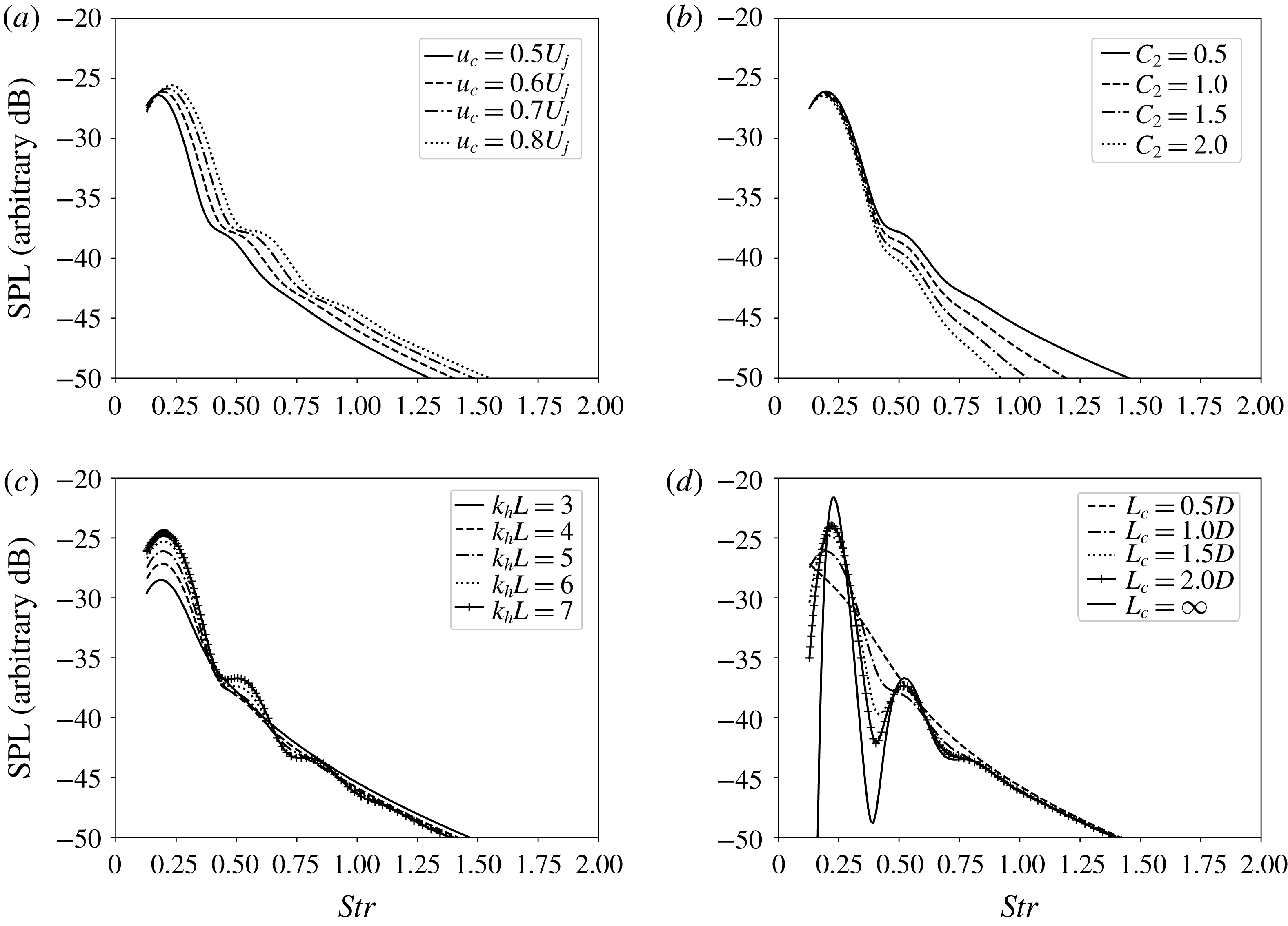
Figure 8. Effect of modelling variables on the acoustic power spectrum when (a) changing convection velocity
 $u_{c}$
, (b) changing amplitude width
$u_{c}$
, (b) changing amplitude width
 $C_{2}$
, (c) changing wavepacket envelope length scale
$C_{2}$
, (c) changing wavepacket envelope length scale
 $L$
, (d) changing coherence-decay length scale
$L$
, (d) changing coherence-decay length scale
 $L_{c}$
for an observation angle of
$L_{c}$
for an observation angle of
 $\unicode[STIX]{x1D703}=150^{0}$
at a distance of
$\unicode[STIX]{x1D703}=150^{0}$
at a distance of
 $100D$
. The modelled jet is operating at a nozzle pressure ratio of
$100D$
. The modelled jet is operating at a nozzle pressure ratio of
 $NPR=3.4$
.
$NPR=3.4$
.
Table 1. Constant values for each parameter used in proposed model.
As expected, we notice that varying the values of each modelling parameter changes the shape of the acoustic spectrum produced. Increasing the convection velocity
 $u_{c}$
shifts the peak frequency to higher Strouhal values as shown in figure 8(a). The rapid drop-off at high Strouhal values from increasing
$u_{c}$
shifts the peak frequency to higher Strouhal values as shown in figure 8(a). The rapid drop-off at high Strouhal values from increasing
 $C_{2}$
in figure 8(b) corresponds to the growing exponential decay as
$C_{2}$
in figure 8(b) corresponds to the growing exponential decay as
 $C_{2}$
increases. While it can be seen that
$C_{2}$
increases. While it can be seen that
 $u_{c}$
and
$u_{c}$
and
 $C_{2}$
do alter the far-field sound spectrum, their effects on the harmonic peaks remain minimal.
$C_{2}$
do alter the far-field sound spectrum, their effects on the harmonic peaks remain minimal.
We note, however, the two length scales characterising the wavepacket do have a more significant effect on the higher-order peaks. From figure 8(c,d), neither
 $L$
nor
$L$
nor
 $L_{c}$
alters the peak frequency predicted. We note that for a large spatial wavepacket envelope (
$L_{c}$
alters the peak frequency predicted. We note that for a large spatial wavepacket envelope (
 $L$
) the peak sound amplitude increases but the artificial peaks become more apparent. As we decrease the value of
$L$
) the peak sound amplitude increases but the artificial peaks become more apparent. As we decrease the value of
 $L$
, the peaks are suppressed; similar to the impact we see with using a finite value of
$L$
, the peaks are suppressed; similar to the impact we see with using a finite value of
 $L_{c}$
in figure 8(d).
$L_{c}$
in figure 8(d).
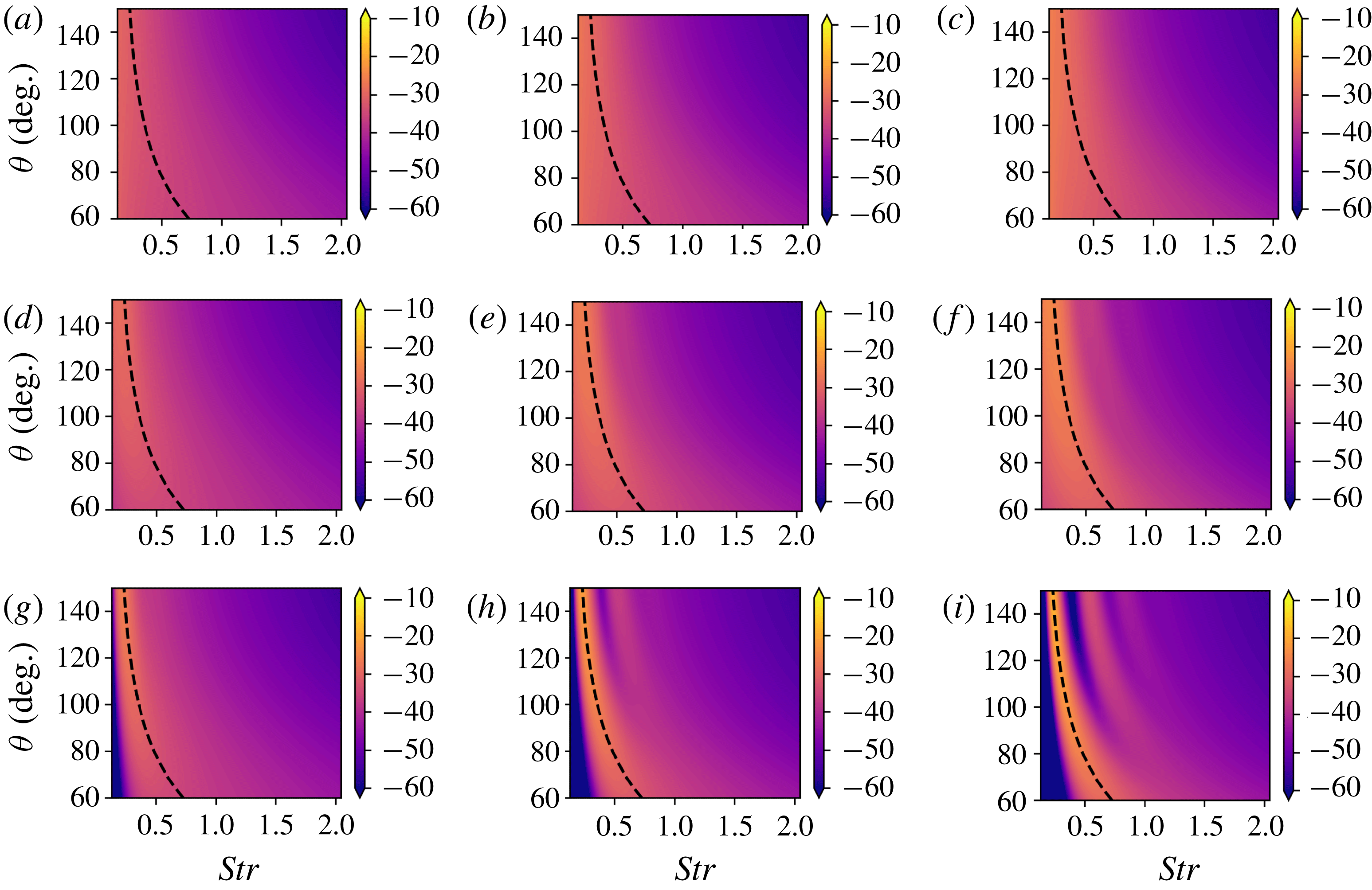
Figure 9. Contours of sound pressure level (arbitrary dB) as a function of frequency (
 $St$
) and directivity (
$St$
) and directivity (
 $\unicode[STIX]{x1D703}$
) for a range of
$\unicode[STIX]{x1D703}$
) for a range of
 $L_{c}$
and
$L_{c}$
and
 $L$
. Each row corresponds to the two-point model with constant value of
$L$
. Each row corresponds to the two-point model with constant value of
 $L_{c}$
; (a–c)
$L_{c}$
; (a–c)
 $L_{c}=0.5D$
, (d–f)
$L_{c}=0.5D$
, (d–f)
 $L_{c}=1.0D$
, (g–i)
$L_{c}=1.0D$
, (g–i)
 $L_{c}=\infty$
. Each column corresponds to the two-point model with constant value of
$L_{c}=\infty$
. Each column corresponds to the two-point model with constant value of
 $k_{h}L$
;
$k_{h}L$
;
 $k_{h}L=3.0$
(a,d,g),
$k_{h}L=3.0$
(a,d,g),
 $k_{h}L=5.0$
(b,e,h) and
$k_{h}L=5.0$
(b,e,h) and
 $k_{h}L=7.0$
(c,f,i). The modelled jet is operating at a nozzle pressure ratio of
$k_{h}L=7.0$
(c,f,i). The modelled jet is operating at a nozzle pressure ratio of
 $NPR=3.4$
.
$NPR=3.4$
.
To further investigate the relationship between
 $L$
and
$L$
and
 $L_{c}$
and their effect with respect to directivity, a set of sound pressure contours is presented in figure 9. The dependency of peak frequency on directivity is lost for small values of
$L_{c}$
and their effect with respect to directivity, a set of sound pressure contours is presented in figure 9. The dependency of peak frequency on directivity is lost for small values of
 $L$
and
$L$
and
 $L_{c}$
. Increasing
$L_{c}$
. Increasing
 $L$
seems to make the BBSAN peak more prominent for all directivity angles and is consistent with previous findings on the effect of spatial modulation of wavepackets (Cavalieri et al.
Reference Cavalieri, Jordan, Agarwal and Gervais2011, Reference Cavalieri, Jordan, Colonius and Gervais2012). The non-compact nature of wavepackets explains, for example, the axisymmetric superdirective radiation of low Mach number turbulent jets (Laufer Reference Laufer1983). In supersonic flows, this can be seen in the directivity dependence of the peak sound-emission frequency.
$L$
seems to make the BBSAN peak more prominent for all directivity angles and is consistent with previous findings on the effect of spatial modulation of wavepackets (Cavalieri et al.
Reference Cavalieri, Jordan, Agarwal and Gervais2011, Reference Cavalieri, Jordan, Colonius and Gervais2012). The non-compact nature of wavepackets explains, for example, the axisymmetric superdirective radiation of low Mach number turbulent jets (Laufer Reference Laufer1983). In supersonic flows, this can be seen in the directivity dependence of the peak sound-emission frequency.
As found by Cavalieri et al. (Reference Cavalieri, Jordan, Colonius and Gervais2012), for superdirectivity to occur, the wavepacket source must not be compact; the condition of
 $k_{h}L\gg 1$
must be met. For BBSAN, the peak frequency also exhibits a directivity dependence (Harper-Bourne & Fisher Reference Harper-Bourne and Fisher1973). Hence, even though by decreasing the value of
$k_{h}L\gg 1$
must be met. For BBSAN, the peak frequency also exhibits a directivity dependence (Harper-Bourne & Fisher Reference Harper-Bourne and Fisher1973). Hence, even though by decreasing the value of
 $L$
we get the same effect as including coherence decay, we find that the values which would be found in supersonic shock-containing jets will not be small. Using two-point correlations of near-field pressure from LES data, Suzuki (Reference Suzuki2016) also found that the axial extent of wavepackets extended over several jet diameters.
$L$
we get the same effect as including coherence decay, we find that the values which would be found in supersonic shock-containing jets will not be small. Using two-point correlations of near-field pressure from LES data, Suzuki (Reference Suzuki2016) also found that the axial extent of wavepackets extended over several jet diameters.
While narrow wavepacket spatial envelopes have been shown in figure 8(c) to suppress the higher-order peaks, the loss of peak frequency directivity (figure 9) and results from previous studies demonstrate that these small, narrow wavepacket envelopes are not plausible. In shock-containing flows, wavepackets are non-compact. Instead, as discussed in § 5, we propose that coherence decay is responsible for smoothing out these higher-order peaks.
Appendix B. Fourier transform of two-point CSD
We present below the result from carrying out the double Fourier transform of equation (2.15):
 $$\begin{eqnarray}\displaystyle & & \displaystyle {\mathcal{F}}(k_{y_{1}},k_{y_{2}})=\frac{1}{8\sqrt{{\displaystyle \frac{1}{L^{2}}}+{\displaystyle \frac{1}{L_{c}^{2}}}}\sqrt{{\displaystyle \frac{2L^{2}+L_{c}^{2}}{L^{4}+L^{2}L_{c}^{2}}}}}\nonumber\\ \displaystyle & & \displaystyle \times \,\left(\right.\!\!\text{e}^{-L^{2}(k_{z}^{2}L^{2}+2k_{h}^{2}L_{c}^{2}-2k_{h}k_{z}L_{c}^{2}+k_{z}^{2}L_{c}^{2}+k_{y}^{2}(L^{2}+L_{c}^{2})+2k_{s}^{2}(2L^{2}+L_{c}^{2})-2k_{s}(k_{y}+k_{z})(2L^{2}+L_{c}^{2})+2k_{y}(k_{z}L^{2}+k_{h}L_{c}^{2}))/4(2L^{2}+L_{c}^{2})}\nonumber\\ \displaystyle & & \displaystyle +\,\text{e}^{-L^{2}(k_{z}^{2}L^{2}+2k_{h}^{2}L_{c}^{2}-2k_{h}k_{z}L_{c}^{2}+k_{z}^{2}L_{c}^{2}+k_{y}^{2}(L^{2}+L_{c}^{2})+2k_{s}^{2}(2L^{2}+L_{c}^{2})+2k_{s}(k_{y}+k_{z})(2L^{2}+L_{c}^{2})+2k_{y}(k_{z}L^{2}+k_{h}L_{c}^{2}))/4(2L^{2}+L_{c}^{2})}\nonumber\\ \displaystyle & & \displaystyle +\,\text{e}^{-L^{2}(2(k_{h}-k_{s})^{2}L_{c}^{2}+2(-k_{h}+k_{s})k_{z}L_{c}^{2}+k_{y}^{2}(L^{2}+L_{c}^{2})+k_{z}^{2}(L^{2}+L_{c}^{2})+2k_{y}(k_{z}L^{2}+(k_{h}-k_{s})L_{c}^{2}))/4(2L^{2}+L_{c}^{2})}\nonumber\\ \displaystyle & & \displaystyle +\,\text{e}^{-L^{2}(2(k_{h}+k_{s})^{2}L_{c}^{2}-2(k_{h}+k_{s})k_{z}L_{c}^{2}+k_{y}^{2}(L^{2}+L_{c}^{2})+k_{z}^{2}(L^{2}+L_{c}^{2})+2k_{y}(k_{z}L^{2}+(k_{h}+k_{s})L_{c}^{2}))/4(2L^{2}+L_{c}^{2})}\left.\!\!\right).\end{eqnarray}$$


