1 Introduction
The quasi-steady (QS) concept of near-wall turbulence is based on the proposition that the statistical properties velocity and second moments, in particular, are universal functions of the distance from the wall,
 $y^{+}$
, i.e. independent of the Reynolds number, provided the variables in question are scaled by the local, instantaneous, wall-shear stress that arises from footprints of the Reynolds-number-dependent ‘large-scale’ turbulent fluctuations in the outer part of the log layer. Here, the definition of ‘large’ and ‘small’ is left open for the time being, as this distinction depends on the method used for scale separation. The QS concept implies that the characteristic time scale of the large-scale component of the velocity field is large as compared to the characteristic time scale of the small-scale component of the velocity field.
$y^{+}$
, i.e. independent of the Reynolds number, provided the variables in question are scaled by the local, instantaneous, wall-shear stress that arises from footprints of the Reynolds-number-dependent ‘large-scale’ turbulent fluctuations in the outer part of the log layer. Here, the definition of ‘large’ and ‘small’ is left open for the time being, as this distinction depends on the method used for scale separation. The QS concept implies that the characteristic time scale of the large-scale component of the velocity field is large as compared to the characteristic time scale of the small-scale component of the velocity field.
An early formalism that broadly pertains to the QS concept, although without resorting to local scaling in the sense described in the above paragraph, is an empirical relationship proposed by Mathis, Hutchins & Marusic (Reference Mathis, Hutchins and Marusic2011) for the streamwise fluctuations only. The proposal is that the actual fluctuations can be recovered from two additive contributions,
 $u^{+}(y^{+})=f_{1}(y^{+},u_{0,ls}^{+})u^{\ast }(y^{+})+f_{2}(y^{+})u_{0,ls}^{+}$
, in which the first is a modulated form of the universal fluctuation,
$u^{+}(y^{+})=f_{1}(y^{+},u_{0,ls}^{+})u^{\ast }(y^{+})+f_{2}(y^{+})u_{0,ls}^{+}$
, in which the first is a modulated form of the universal fluctuation,
 $u^{\ast }(y^{+})$
, unaffected by outer large-scale fluctuations, identified by (
$u^{\ast }(y^{+})$
, unaffected by outer large-scale fluctuations, identified by (
 $[..]_{ls}$
), and the second is a superposition term that arises from the large-scale streamwise motion at location
$[..]_{ls}$
), and the second is a superposition term that arises from the large-scale streamwise motion at location
 $y^{+}$
, derived from data for the Reynolds-number-dependent large-scale motions at an outer location ‘o’, multiplied by an empirical correlation function
$y^{+}$
, derived from data for the Reynolds-number-dependent large-scale motions at an outer location ‘o’, multiplied by an empirical correlation function
 $f_{2}$
. The empirical function
$f_{2}$
. The empirical function
 $f_{1}$
expresses the fact that the universal quantity is altered (amplified or attenuated) by the modulating action of the large-scale motion. In fact, this equation is a prediction formula for the effects of the Reynolds number on the wall-normal statistics. Although
$f_{1}$
expresses the fact that the universal quantity is altered (amplified or attenuated) by the modulating action of the large-scale motion. In fact, this equation is a prediction formula for the effects of the Reynolds number on the wall-normal statistics. Although
 $u^{\ast }(y^{+})$
would appear to comply with the QS concept, in that is it is supposedly independent of the large-scale motions, it is not strictly compatible with the concept, because it is scaled with the average wall-shear stress.
$u^{\ast }(y^{+})$
would appear to comply with the QS concept, in that is it is supposedly independent of the large-scale motions, it is not strictly compatible with the concept, because it is scaled with the average wall-shear stress.
A formally rigorous application of the QS concept, although again derived only for the streamwise fluctuations and energy, was recently proposed by Zhang & Chernyshenko (Reference Zhang and Chernyshenko2016) in the form of an elegant theoretical framework to which they refer as ‘quasi-steady quasi-homogeneous (QSQH) theory’. The corner stone of the theory, limited to the streamwise velocity statistics in the near-wall layer
 $y^{+}<80$
, is the assumption that the total turbulent velocity
$y^{+}<80$
, is the assumption that the total turbulent velocity
 $u(t,x,y,z)$
yields universal statistics if it is considered (or sampled) on the surface
$u(t,x,y,z)$
yields universal statistics if it is considered (or sampled) on the surface
 $(t^{+,ls},x^{+,ls},y^{+,ls},z^{+,ls})$
and normalised by
$(t^{+,ls},x^{+,ls},y^{+,ls},z^{+,ls})$
and normalised by
 $u_{\unicode[STIX]{x1D70F},ls}$
, where the superscript
$u_{\unicode[STIX]{x1D70F},ls}$
, where the superscript
 $ls$
indicates scaling by the local, instantaneous, large-scale wall-shear stress
$ls$
indicates scaling by the local, instantaneous, large-scale wall-shear stress
 $u_{\unicode[STIX]{x1D70F},ls}=\sqrt{\unicode[STIX]{x1D707}/\unicode[STIX]{x1D70C}}\times \sqrt{(\text{d}u_{ls}/\text{d}y)_{y=0}}$
. This scaling is thus held to take account naturally of the modulation and superposition, expressed by
$u_{\unicode[STIX]{x1D70F},ls}=\sqrt{\unicode[STIX]{x1D707}/\unicode[STIX]{x1D70C}}\times \sqrt{(\text{d}u_{ls}/\text{d}y)_{y=0}}$
. This scaling is thus held to take account naturally of the modulation and superposition, expressed by
 $f_{1}$
and
$f_{1}$
and
 $f_{2}$
, respectively, in Mathis et al.’s prediction formula. Zhang & Chernyshenko (Reference Zhang and Chernyshenko2016) adopt a particular Fourier-filtering approach to separating the large-scale and small-scale motions, and they show, by reference to linear expansions for the correlations
$f_{2}$
, respectively, in Mathis et al.’s prediction formula. Zhang & Chernyshenko (Reference Zhang and Chernyshenko2016) adopt a particular Fourier-filtering approach to separating the large-scale and small-scale motions, and they show, by reference to linear expansions for the correlations
 $\langle u_{ls}u_{ls}\rangle$
and
$\langle u_{ls}u_{ls}\rangle$
and
 $\langle u_{\unicode[STIX]{x1D70F},ls}u_{ss}^{2}\rangle$
, subject to relatively weak large-scale fluctuations and the subscript
$\langle u_{\unicode[STIX]{x1D70F},ls}u_{ss}^{2}\rangle$
, subject to relatively weak large-scale fluctuations and the subscript
 $ss$
denoting small-scale fluctuations, that the functions
$ss$
denoting small-scale fluctuations, that the functions
 $f_{1}$
and
$f_{1}$
and
 $f_{2}$
can be derived analytically from the theory, although the theory itself does not explicitly presume the existence of superposition, relying only on approximations to correlations involving the amplitude modulation
$f_{2}$
can be derived analytically from the theory, although the theory itself does not explicitly presume the existence of superposition, relying only on approximations to correlations involving the amplitude modulation
 $\langle u_{\unicode[STIX]{x1D70F},ls}u_{ss}^{2}\rangle$
. As the QS concept is general, it should be possible, in principle, to extend the theory to statistical quantities other than the streamwise stress. While this remains to be done, it is certainly possible to examine the validity of the concept by scrutinising direct numerical simulation (DNS) data, as done herein.
$\langle u_{\unicode[STIX]{x1D70F},ls}u_{ss}^{2}\rangle$
. As the QS concept is general, it should be possible, in principle, to extend the theory to statistical quantities other than the streamwise stress. While this remains to be done, it is certainly possible to examine the validity of the concept by scrutinising direct numerical simulation (DNS) data, as done herein.
A corollary of the QS concept – referred to as ‘the QSQH hypothesis per se’ in Zhang & Chernyshenko (Reference Zhang and Chernyshenko2016), in contrast to ‘the QSQH re-universality hypothesis’ – is that the near-wall statistics, when conditionally scaled with the skin friction derived from the large-scale footprints, should be universal at any condition value of the wall-shear stress. More specifically, universality should apply equally to both positive and negative large-scale footprints. Based on a statistical analysis of DNS data at
 $Re_{\unicode[STIX]{x1D70F}}=1000$
, it is shown in this paper that scaling with the local, large-scale footprints, compatible with the QS theory, is not universal beyond a very limited distance from the wall. It is further demonstrated that the lack of universality beyond
$Re_{\unicode[STIX]{x1D70F}}=1000$
, it is shown in this paper that scaling with the local, large-scale footprints, compatible with the QS theory, is not universal beyond a very limited distance from the wall. It is further demonstrated that the lack of universality beyond
 $y^{+}\approx 80$
, manifesting itself by major differences in the statistics that are conditional on large negative and positive skin-friction footprints, is due to distortions in the mean strain and corresponding variations in the shear-driven production in the outer region. These affect not only the outer region, but also to a more limited extent, the inner-layer statistics.
$y^{+}\approx 80$
, manifesting itself by major differences in the statistics that are conditional on large negative and positive skin-friction footprints, is due to distortions in the mean strain and corresponding variations in the shear-driven production in the outer region. These affect not only the outer region, but also to a more limited extent, the inner-layer statistics.
In an earlier paper by the authors (Agostini & Leschziner Reference Agostini and Leschziner2016), the authors investigate the validity of the QS concept for channel flow at
 $Re_{\unicode[STIX]{x1D70F}}\approx 4200$
using data by Lozano-Durán & Jiménez (Reference Lozano-Durán and Jiménez2014). The present paper adopts a formally more rigorous statistical approach to extracting relevant statistical data from our own simulations at
$Re_{\unicode[STIX]{x1D70F}}\approx 4200$
using data by Lozano-Durán & Jiménez (Reference Lozano-Durán and Jiménez2014). The present paper adopts a formally more rigorous statistical approach to extracting relevant statistical data from our own simulations at
 $Re_{\unicode[STIX]{x1D70F}}\approx 1000$
, and extends the earlier work by including results that illuminate the origin of departures from the QS concept. The present examination also complements, though is distinct from, the study of Agostini & Leschziner (Reference Agostini and Leschziner2019), which aims squarely at identifying the physical mechanisms that are responsible for the modulation of small-scale turbulence by larger scales in the same channel flow considered herein.
$Re_{\unicode[STIX]{x1D70F}}\approx 1000$
, and extends the earlier work by including results that illuminate the origin of departures from the QS concept. The present examination also complements, though is distinct from, the study of Agostini & Leschziner (Reference Agostini and Leschziner2019), which aims squarely at identifying the physical mechanisms that are responsible for the modulation of small-scale turbulence by larger scales in the same channel flow considered herein.
2 Data processing
The data used herein have been described in several earlier papers (Agostini & Leschziner Reference Agostini and Leschziner2018), and this included a demonstration of their accuracy by reference to several quality indicators. In brief, the simulations were performed over a box of length, height and depth of
 $12h\times 2h\times 6h$
, respectively, corresponding to approximately
$12h\times 2h\times 6h$
, respectively, corresponding to approximately
 $(12\times 2\times 6)\times 10^{3}$
wall units. The box was covered with a finite-volume mesh of
$(12\times 2\times 6)\times 10^{3}$
wall units. The box was covered with a finite-volume mesh of
 $1056\times 528\times 1056\;(=589\times 10^{6})$
cells. The corresponding cell dimensions were
$1056\times 528\times 1056\;(=589\times 10^{6})$
cells. The corresponding cell dimensions were
 $(x^{+},y_{min}^{+},y_{max}^{+},z^{+})=(11.4,0.4,7.2,5.7)$
.
$(x^{+},y_{min}^{+},y_{max}^{+},z^{+})=(11.4,0.4,7.2,5.7)$
.
The separation between large and small scales was effected with the empirical mode decomposition (EMD) (Huang et al.
Reference Huang, Shen, Long, Wu, Shih, Zheng, Yen, Tung and Liu1998). The method originates from signal processing of temporally evolving functions, and the present authors have adapted it to two-dimensional spatial fields (Agostini & Leschziner Reference Agostini and Leschziner2014), exploiting it to investigate a range of scale-interaction issues for canonical and forced channel flows (Agostini & Leschziner Reference Agostini and Leschziner2014, Reference Agostini and Leschziner2018). The application of the method to all wall-parallel two-dimensional fields of any full-volume numerical snapshot yields a three-dimensional decomposition of the turbulence field. In essence, the method splits any field into several EMD modes – six in the present case – each associated with a relatively narrow band of scales. Here, as in previous studies by the present authors, the large-scale field is deemed represented by modes 4, 5 and 6, the small-scale field by modes 1 and 2, and an intermediate-scale field by mode 3. A justification for this attribution is given in Agostini & Leschziner (Reference Agostini and Leschziner2018) by reference to premultiplied spectra for the EMD modes, relative to the spectra of the whole field. As an illustrative example, figure 1 shows the premultiplied spanwise spectra for the total skin-friction fluctuations and its small-scale and large-scale components. A subtle point to convey in relation to these spectra is that the small-scale and large-scale EMD modes for the skin friction are weakly correlated. This emerges from the joint probability density function (p.d.f.) given in figure 1(b), which is, essentially, representative of the corresponding skin-friction fluctuations. The p.d.f. is seen to be asymmetric (skewed), implying a negative correlation, which is indeed the case. This correlation reflects the fact that the positive modulation – the relationship between the large-scale fluctuations and the envelope of the small-scale variance or intensity – becomes asymmetric as the small-scale intensity strengthens, due to splatting causing a reorientation of fluctuations from the streamwise to the spanwise direction (Agostini & Leschziner Reference Agostini and Leschziner2014). The correlation thus manifests itself by a finite level of the energy density formed with small-scale and large-scale fluctuations (denoted by
 $\unicode[STIX]{x1D719}_{ss,ls}$
in figure 1). With this contribution accounted for, the spectra demonstrate that, while the two scales are not cleanly separated in a spectral sense at this relatively low Reynolds number, the large-scale/small-scale boundary is at
$\unicode[STIX]{x1D719}_{ss,ls}$
in figure 1). With this contribution accounted for, the spectra demonstrate that, while the two scales are not cleanly separated in a spectral sense at this relatively low Reynolds number, the large-scale/small-scale boundary is at
 $\unicode[STIX]{x1D706}_{z}^{+}\approx 500$
, with the large scale dominant beyond
$\unicode[STIX]{x1D706}_{z}^{+}\approx 500$
, with the large scale dominant beyond
 $\unicode[STIX]{x1D706}_{z}^{+}>700$
. The small-scale peak occurs at
$\unicode[STIX]{x1D706}_{z}^{+}>700$
. The small-scale peak occurs at
 $\unicode[STIX]{x1D706}_{z}^{+}\approx 100$
, indicative of the inter-streak distance in the buffer layer.
$\unicode[STIX]{x1D706}_{z}^{+}\approx 100$
, indicative of the inter-streak distance in the buffer layer.

Figure 1. Scale separation by the empirical mode decomposition; (a) premultiplied spanwise spectra of small-scale and large-scale streamwise energy density; subscripts
 $tt$
,
$tt$
,
 $ss$
and
$ss$
and
 $ls$
denote total, small-scale and large-scale energy-density components, respectively; for the significance of the mixed
$ls$
denote total, small-scale and large-scale energy-density components, respectively; for the significance of the mixed
 $ss,ls$
component, see text; (b) joint p.d.f. of small-scale and large-scale velocity fluctuations at
$ss,ls$
component, see text; (b) joint p.d.f. of small-scale and large-scale velocity fluctuations at
 $y^{+}=0.2$
, illuminating the correlation between the two fluctuation fields and the origin of the mixed spectral component
$y^{+}=0.2$
, illuminating the correlation between the two fluctuation fields and the origin of the mixed spectral component
 $\unicode[STIX]{x1D6F7}_{ss,ls}$
.
$\unicode[STIX]{x1D6F7}_{ss,ls}$
.

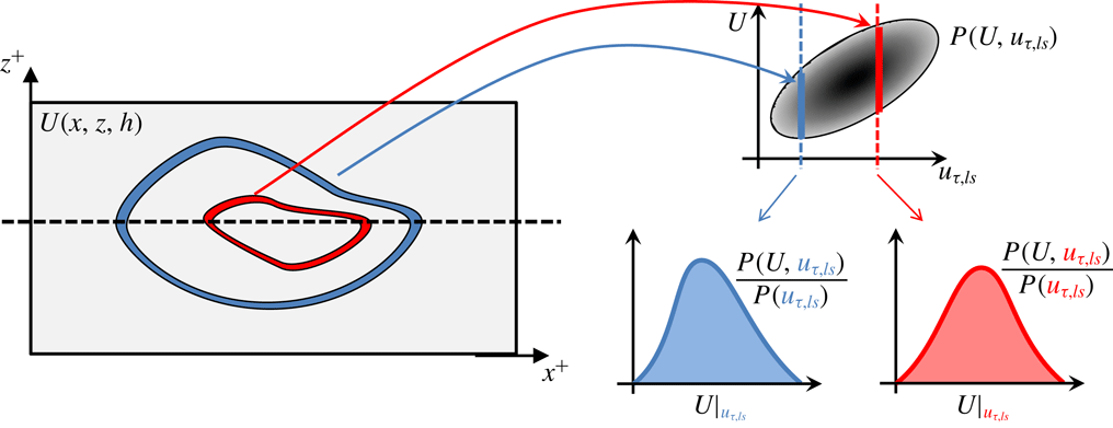
Figure 2. Conceptual representation of the data-extraction process across any wall-normal plane
 $y_{j}$
.
$y_{j}$
.
The manner in which relevant statistical results have been extracted from the data is explained below, for the particular case of the streamwise velocity component,
 $U$
, with support from the sketches in figure 2. It is remarked that the process below may be applied to any other fluctuating variable.
$U$
, with support from the sketches in figure 2. It is remarked that the process below may be applied to any other fluctuating variable.
(i) Across any wall-parallel plane,
 $y_{j}$
, pairs of
$(U(x-\unicode[STIX]{x0394}x,z),u_{\unicode[STIX]{x1D70F},ls}(x,z))$
are recorded, where
$\unicode[STIX]{x0394}x$
represents a plane-specific shift that is prescribed by the
$y$
-wise variation of the locus of maximum correlation between
$U$
and
$u_{\unicode[STIX]{x1D70F},ls}$
(generally, referred as the ‘lag’ in the literature). This allows the joint p.d.f.
$P(U,u_{\unicode[STIX]{x1D70F},ls})$
to be derived. For each value
$u_{\unicode[STIX]{x1D70F},ls}$
, there is also a value
$y_{j}^{+,ls}=y_{j}^{+}\times (u_{\unicode[STIX]{x1D70F},ls}/u_{\unicode[STIX]{x1D70F}})$
and a value of the local skin friction
$Cf_{ls}$
.
$y_{j}$
, pairs of
$(U(x-\unicode[STIX]{x0394}x,z),u_{\unicode[STIX]{x1D70F},ls}(x,z))$
are recorded, where
$\unicode[STIX]{x0394}x$
represents a plane-specific shift that is prescribed by the
$y$
-wise variation of the locus of maximum correlation between
$U$
and
$u_{\unicode[STIX]{x1D70F},ls}$
(generally, referred as the ‘lag’ in the literature). This allows the joint p.d.f.
$P(U,u_{\unicode[STIX]{x1D70F},ls})$
to be derived. For each value
$u_{\unicode[STIX]{x1D70F},ls}$
, there is also a value
$y_{j}^{+,ls}=y_{j}^{+}\times (u_{\unicode[STIX]{x1D70F},ls}/u_{\unicode[STIX]{x1D70F}})$
and a value of the local skin friction
$Cf_{ls}$
.(ii) For each value
$u_{\unicode[STIX]{x1D70F},ls}$
, the conditional first and second moments may now be determined by integrating the conditional p.d.f., premultiplied by
$U$
or
$UU$
, respectively, i.e., (2.1)$$\begin{eqnarray}\displaystyle & \displaystyle \overline{U}|_{u_{\unicode[STIX]{x1D70F},ls}}=\int _{-\infty }^{+\infty }U\frac{P(U,u_{\unicode[STIX]{x1D70F},ls})}{P(u_{\unicode[STIX]{x1D70F},ls})}\,\text{d}U & \displaystyle\end{eqnarray}$$
(2.2)For each value$$\begin{eqnarray}\displaystyle & \displaystyle \overline{uu}|_{u_{\unicode[STIX]{x1D70F},ls}}=\int _{-\infty }^{+\infty }UU\frac{P(U,u_{\unicode[STIX]{x1D70F},ls})}{P(u_{\unicode[STIX]{x1D70F},ls})}\,\text{d}U-(\overline{U}|_{u_{\unicode[STIX]{x1D70F},ls}})^{2}. & \displaystyle\end{eqnarray}$$
$u_{\unicode[STIX]{x1D70F},ls}$
– or, equivalently, skin friction
$Cf_{ls}$
– there is, therefore, a conditional mean value
$\overline{U}|_{u_{\unicode[STIX]{x1D70F},ls}}$
and standard deviation
$\overline{uu}|_{u_{\unicode[STIX]{x1D70F},ls}}$
in conjunction with a corresponding value
$y_{j}^{+,ls}$
.(iii) The above steps are repeated for all
$y^{+}$
. This allows maps of the form
$\overline{u_{i}u_{j}}|_{u_{\unicode[STIX]{x1D70F},ls}}=f(Cf_{ls},y^{+,ls})$
to be constructed for any statistical variable (for example, (2.1) and (2.2)).


With the fields of the conditional variables thus determined, it is now possible to examine the variations of the variables as functions of
 $y^{+,ls}$
and
$y^{+,ls}$
and
 $Cf_{ls}$
. This is the focus of the examination in the following section.
$Cf_{ls}$
. This is the focus of the examination in the following section.
3 Results and discussion
Profiles of the total streamwise, shear and spanwise stresses at the five conditions marked in the p.d.f. of the large-scale skin friction given in figure 3 are shown in figure 4, the subscript
 $tt$
identifying the total fluctuations, as opposed to the decomposed large-scale/small-scale components. The p.d.f.
$tt$
identifying the total fluctuations, as opposed to the decomposed large-scale/small-scale components. The p.d.f.
 $P(Cf_{ls})$
conveys the fact that, notwithstanding the relatively low Reynolds number, the footprints of the large-scale motions are substantial, giving rise to skin-friction fluctuations that exceed 50 % of the mean. All three stress components are scaled in figure 4(a,c,e) by the mean shear velocity and in figure 4(b,d,f) by the local large-scale shear velocity, with the latter presumed to return a universal behaviour that reflects the QS concept.
$P(Cf_{ls})$
conveys the fact that, notwithstanding the relatively low Reynolds number, the footprints of the large-scale motions are substantial, giving rise to skin-friction fluctuations that exceed 50 % of the mean. All three stress components are scaled in figure 4(a,c,e) by the mean shear velocity and in figure 4(b,d,f) by the local large-scale shear velocity, with the latter presumed to return a universal behaviour that reflects the QS concept.

Figure 3. The p.d.f. of large-scale skin-friction fluctuations; the magenta line corresponds to the median value of the p.d.f..
Two distinctive features in the profiles scaled by the mean wall-shear stress (figure 4
a,c,e) are, first, the strong same-signed dependence of the stress levels in the buffer layer on the footprints and, second, the opposite-signed dependence of the
 $y^{+}$
location of the maxima on the footprints. It is not possible to link, unambiguously, either feature to superposition or modulation, as defined by Mathis et al. (Reference Mathis, Hutchins and Marusic2011). However, as the stress levels in the buffer layer are dominated by small-scale activity – as will be demonstrated later – the increase in the stresses, especially the maxima in the streamwise stress, may be broadly equated with modulation. The fact that the maxima shift towards the wall as the skin friction increases, and vice versa, might superficially be interpreted as being the consequence of wall-normal convective motions induced by large-scale sweeps and ejections associated with footprinting. However, if the QS concept is valid, these shifts merely reflect the fact that the turbulence state adjusts itself rapidly to the relatively slow large-scale motions (and footprints), in which case local scaling of
$y^{+}$
location of the maxima on the footprints. It is not possible to link, unambiguously, either feature to superposition or modulation, as defined by Mathis et al. (Reference Mathis, Hutchins and Marusic2011). However, as the stress levels in the buffer layer are dominated by small-scale activity – as will be demonstrated later – the increase in the stresses, especially the maxima in the streamwise stress, may be broadly equated with modulation. The fact that the maxima shift towards the wall as the skin friction increases, and vice versa, might superficially be interpreted as being the consequence of wall-normal convective motions induced by large-scale sweeps and ejections associated with footprinting. However, if the QS concept is valid, these shifts merely reflect the fact that the turbulence state adjusts itself rapidly to the relatively slow large-scale motions (and footprints), in which case local scaling of
 $y^{+}$
should remove the shift.
$y^{+}$
should remove the shift.
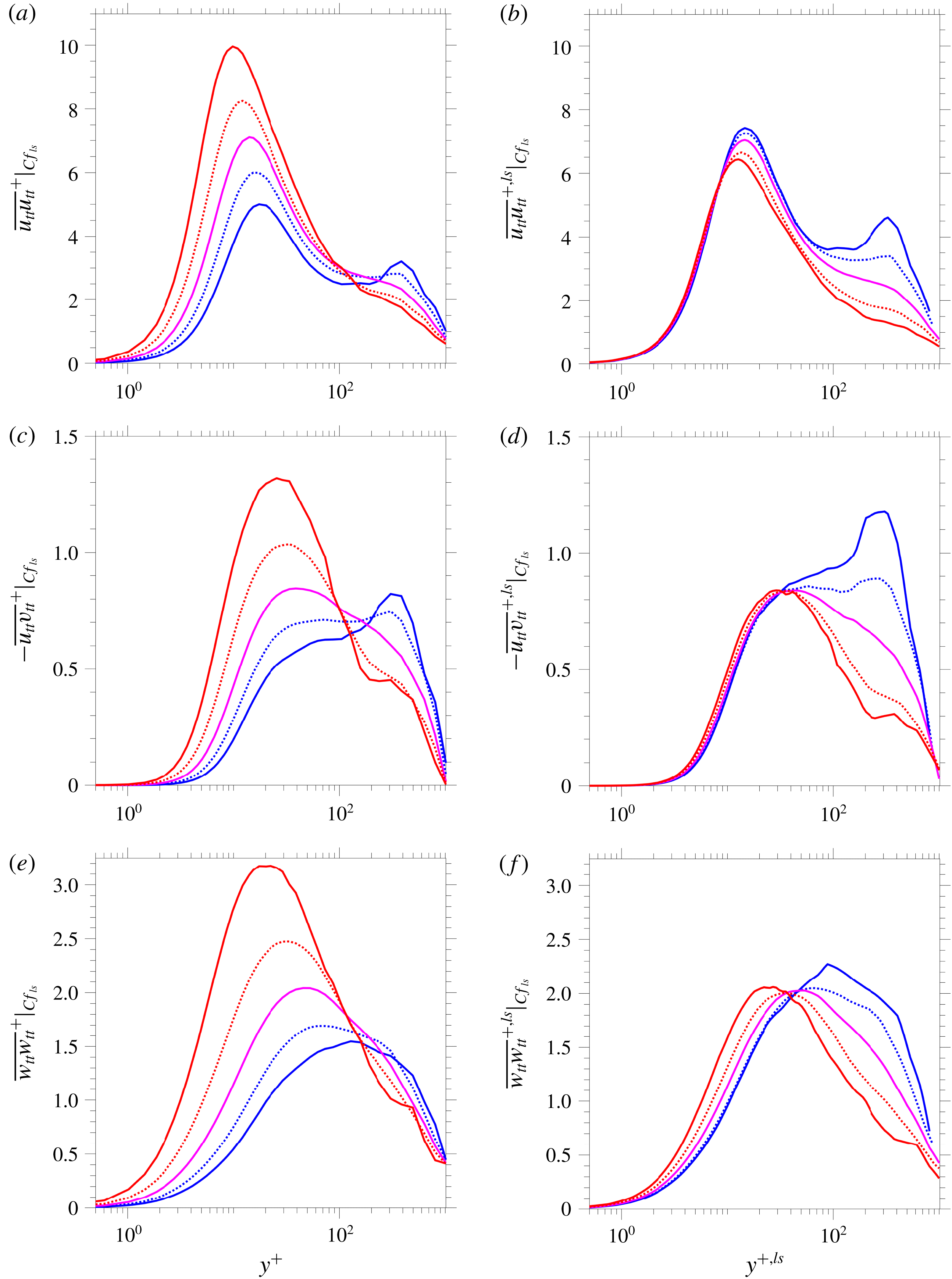


Figure 5. Joint p.d.f.s of streamwise and spanwise fluctuations for (in blue) extreme 5 % negative and (in red) extreme positive 5 % large-scale skin-friction fluctuations; (a) scaling by average wall-shear velocity at
 $y^{+}\approx 10$
; (b) scaling by local wall-shear velocity at
$y^{+}\approx 10$
; (b) scaling by local wall-shear velocity at
 $y_{ls}^{+}\approx 10$
.
$y_{ls}^{+}\approx 10$
.
The locally scaled profiles in figure 4 feature a partial collapse close to the wall, thus supporting, to a fair degree, the QS concept upon which Zhang & Chernyshenko’s theory is based. However, the approximate collapse in the profiles is confined to the relatively thin layer
 $y^{+,ls}<80$
, a limitation that Zhang & Chernyshenko accept in their theory. The collapse of the profiles for
$y^{+,ls}<80$
, a limitation that Zhang & Chernyshenko accept in their theory. The collapse of the profiles for
 $\overline{u_{tt}u_{tt}}$
is only partially satisfied closer to the wall, in the range down to
$\overline{u_{tt}u_{tt}}$
is only partially satisfied closer to the wall, in the range down to
 $10<y^{+,ls}<80$
, and this is a feature that will be expanded on below by reference to results for shear production. The collapse of the spanwise-stress profiles,
$10<y^{+,ls}<80$
, and this is a feature that will be expanded on below by reference to results for shear production. The collapse of the spanwise-stress profiles,
 $\overline{w_{tt}w_{tt}}$
, is rather poor, even close to the wall, and there are reasons to believe that this is connected to distortions provoked by ‘splatting’ and ‘anti-splatting’ that accompanies large-scale sweeps and ejections, respectively.
$\overline{w_{tt}w_{tt}}$
, is rather poor, even close to the wall, and there are reasons to believe that this is connected to distortions provoked by ‘splatting’ and ‘anti-splatting’ that accompanies large-scale sweeps and ejections, respectively.
Evidence for the role played by splatting in causing the above distortions is provided by the joint
 $(u_{tt},w_{tt})$
-p.d.f.s in figure 5. In both plots, the blue contours are conditional on the lowest 5 % of
$(u_{tt},w_{tt})$
-p.d.f.s in figure 5. In both plots, the blue contours are conditional on the lowest 5 % of
 $Cf_{ls}$
, while the red contours are conditional on the top 5 % of
$Cf_{ls}$
, while the red contours are conditional on the top 5 % of
 $Cf_{ls}$
. The difference between the two plots lies in the scaling: in figure 5(a) the fluctuations in
$Cf_{ls}$
. The difference between the two plots lies in the scaling: in figure 5(a) the fluctuations in
 $P(u_{tt}^{+},w_{tt}^{+})$
are scaled by the mean wall-shear velocity and the fluctuations are sampled at
$P(u_{tt}^{+},w_{tt}^{+})$
are scaled by the mean wall-shear velocity and the fluctuations are sampled at
 $y^{+}\approx 10$
, while in figure 5(b), for
$y^{+}\approx 10$
, while in figure 5(b), for
 $P(u_{tt}^{+,ls},w_{tt}^{+,ls})$
, scaling is effected with the local large-scale wall-shear velocity, and the fluctuations are sampled at
$P(u_{tt}^{+,ls},w_{tt}^{+,ls})$
, scaling is effected with the local large-scale wall-shear velocity, and the fluctuations are sampled at
 $y^{+,ls}\approx 10$
. It is emphasised that the constant value of
$y^{+,ls}\approx 10$
. It is emphasised that the constant value of
 $y^{+,ls}$
means that sampling is, in effect, performed on a curved surface intersecting several
$y^{+,ls}$
means that sampling is, in effect, performed on a curved surface intersecting several
 $y^{+}=\text{const.}$
planes in the
$y^{+}=\text{const.}$
planes in the
 $x,y,z$
system, rather than on a single
$x,y,z$
system, rather than on a single
 $y$
-plane. The p.d.f. contours in figure 5(a) provide visually striking evidence of the very different conditions at negative and positive footprints, with the red contours depicting far more intense streamwise as well as spanwise fluctuations for extreme positive footprints in the nominal buffer layer, in line with figures 4(a) and 4(e). Figure 5(b) pertains specifically to the QS concept, relating to figure 4(f), in particular. Consistent with earlier observations on the validity of the QS concept for streamwise fluctuations close to the wall, the contours in figure 5(b) virtually collapse at low spanwise fluctuations, and they also do so when
$y$
-plane. The p.d.f. contours in figure 5(a) provide visually striking evidence of the very different conditions at negative and positive footprints, with the red contours depicting far more intense streamwise as well as spanwise fluctuations for extreme positive footprints in the nominal buffer layer, in line with figures 4(a) and 4(e). Figure 5(b) pertains specifically to the QS concept, relating to figure 4(f), in particular. Consistent with earlier observations on the validity of the QS concept for streamwise fluctuations close to the wall, the contours in figure 5(b) virtually collapse at low spanwise fluctuations, and they also do so when
 $P(u_{tt}^{+,ls},w_{tt}^{+,ls})$
is integrated over
$P(u_{tt}^{+,ls},w_{tt}^{+,ls})$
is integrated over
 $w_{tt}^{+,ls}$
to yield the one-dimensional p.d.f.
$w_{tt}^{+,ls}$
to yield the one-dimensional p.d.f.
 $P(u_{tt}^{+,ls})$
. In contrast, the blue and red contours differ substantially in the range of positive
$P(u_{tt}^{+,ls})$
. In contrast, the blue and red contours differ substantially in the range of positive
 $u^{+,ls}$
values in which the spanwise fluctuations
$u^{+,ls}$
values in which the spanwise fluctuations
 $w_{tt}^{+,ls}$
are high, and this is consistent with the departures shown in figure 4(f). The red contours pertain to the 5 % extreme positive
$w_{tt}^{+,ls}$
are high, and this is consistent with the departures shown in figure 4(f). The red contours pertain to the 5 % extreme positive
 $Cf_{ls}$
values, and are thus associated with large-scale sweeps that cause splatting on the wall, and thus enhanced spanwise fluctuations. The distinctive pear-like shape of the p.d.f. contours indicates that positive streamwise fluctuations go hand-in-hand with increasing splatting intensity as the footprint magnitude rises.
$Cf_{ls}$
values, and are thus associated with large-scale sweeps that cause splatting on the wall, and thus enhanced spanwise fluctuations. The distinctive pear-like shape of the p.d.f. contours indicates that positive streamwise fluctuations go hand-in-hand with increasing splatting intensity as the footprint magnitude rises.
It is pertinent to comment here that Zhang & Chernyshenko (Reference Zhang and Chernyshenko2016) suggest (bottom of § II(A)) that ‘both
 $u$
and
$u$
and
 $u_{\unicode[STIX]{x1D70F}L}$
should actually be considered as vector quantities and the hypothesis should be refined accordingly’. However, this suggestion was neither pursued by Zhang & Chernyshenko, nor was tested herein, except for an ineffective attempt to scale the magnitude of the velocity fluctuation by the magnitude of the large-scale friction velocity. It is possible that a projection of the velocity fluctuations onto the direction of the vector of the large-scale friction velocity might improve the collapse of the spanwise-fluctuations profile, relative to that shown in figure 4, but this remains to be investigated.
$u_{\unicode[STIX]{x1D70F}L}$
should actually be considered as vector quantities and the hypothesis should be refined accordingly’. However, this suggestion was neither pursued by Zhang & Chernyshenko, nor was tested herein, except for an ineffective attempt to scale the magnitude of the velocity fluctuation by the magnitude of the large-scale friction velocity. It is possible that a projection of the velocity fluctuations onto the direction of the vector of the large-scale friction velocity might improve the collapse of the spanwise-fluctuations profile, relative to that shown in figure 4, but this remains to be investigated.

Figure 6. Variations in the state of anisotropy in the near-wall region conditional on the large-scale skin friction; (a) map of the one-component (1C)-turbulence metric
 $C_{1c}$
in the barocentric anisotropy triangle; (b) map of the two-component (2C)-turbulence metric
$C_{1c}$
in the barocentric anisotropy triangle; (b) map of the two-component (2C)-turbulence metric
 $C_{2c}$
in the barocentric anisotropy triangle (both vary between 0 and 1, the latter value indicating 1C or 2C state, respectively).
$C_{2c}$
in the barocentric anisotropy triangle (both vary between 0 and 1, the latter value indicating 1C or 2C state, respectively).
Strong variations in the state of the anisotropy depending on the sign and intensity of the footprinting also suggest departures from the QS concept. Such variations are therefore examined in figure 6. This contains maps of two parameters that convey the dependence of the anisotropic state of the velocity fluctuations over the locally scaled wall distance, conditional on the large-scale skin friction. Banerjee et al. (Reference Banerjee, Krahl, Durst and Zenger2007) express the state of anisotropy by three ‘barocentric coordinates’ (vertices) of the ‘barocentric triangle’, characterising the one-component (
 $1$
C), the two-component (
$1$
C), the two-component (
 $2$
C) and the isotropic state of turbulence (
$2$
C) and the isotropic state of turbulence (
 $3$
C), respectively. These coordinates are derived from the eigenvalues of the anisotropic stress tensor, so that every state of the turbulence field is represented by the sum of metrics
$3$
C), respectively. These coordinates are derived from the eigenvalues of the anisotropic stress tensor, so that every state of the turbulence field is represented by the sum of metrics
 $C_{1c}$
,
$C_{1c}$
,
 $C_{2c}$
and the isotropic-state metric (
$C_{2c}$
and the isotropic-state metric (
 $C_{3c}$
) being unity, with any one of the metrics varying between 0 and 1. Figures 6(a) and 6(b) provide maps of the metrics
$C_{3c}$
) being unity, with any one of the metrics varying between 0 and 1. Figures 6(a) and 6(b) provide maps of the metrics
 $C_{1c}$
and
$C_{1c}$
and
 $C_{2c}$
, respectively. In each case, an increasing value towards 1 indicates an increasing trend towards either the 1C or the 2C state. The map for
$C_{2c}$
, respectively. In each case, an increasing value towards 1 indicates an increasing trend towards either the 1C or the 2C state. The map for
 $C_{1c}$
indicates a strong tendency towards the 1C state in the buffer layer – i.e. pronounced streaky structures – for negative footprints, which are associated with large-scale ejections. With increasing skin-friction condition,
$C_{1c}$
indicates a strong tendency towards the 1C state in the buffer layer – i.e. pronounced streaky structures – for negative footprints, which are associated with large-scale ejections. With increasing skin-friction condition,
 $C_{1c}$
declines and
$C_{1c}$
declines and
 $C_{2c}$
increases. This trend towards the 2C state is associated with large-scale sweeps (i.e. stronger splatting), which weaken the 1C streaky structures due a strong increase in
$C_{2c}$
increases. This trend towards the 2C state is associated with large-scale sweeps (i.e. stronger splatting), which weaken the 1C streaky structures due a strong increase in
 $w_{tt}^{+}$
. The trend is thus towards flattening (elongated ‘pancake’-like) structures – a state that is especially pronounced very close to the wall. The fact that the spanwise and streamwise fluctuations vary at different rates with increasing footprint magnitude implies that a recovery of the QS state would require the streamwise and spanwise fluctuations to be scaled by a different value of
$w_{tt}^{+}$
. The trend is thus towards flattening (elongated ‘pancake’-like) structures – a state that is especially pronounced very close to the wall. The fact that the spanwise and streamwise fluctuations vary at different rates with increasing footprint magnitude implies that a recovery of the QS state would require the streamwise and spanwise fluctuations to be scaled by a different value of
 $u_{\unicode[STIX]{x1D70F},ls}$
, which is obviously inconsistent with the QS concept.
$u_{\unicode[STIX]{x1D70F},ls}$
, which is obviously inconsistent with the QS concept.
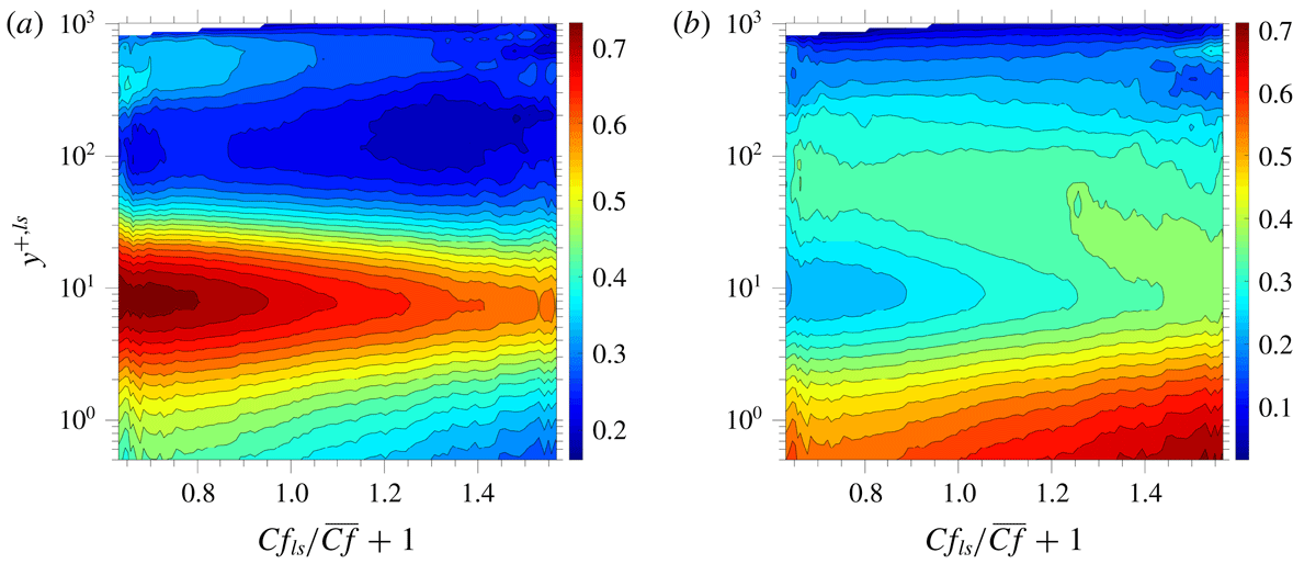
As expected, substantial departures from the QS conditions occur in the outer layer,
 $y^{+,ls}>80$
, the divergence among the profiles peaking around
$y^{+,ls}>80$
, the divergence among the profiles peaking around
 $y^{+,ls}=200$
–300. The reason for this non-universal behaviour emerges from figure 7, which shows a map of the conditional streamwise production rate,
$y^{+,ls}=200$
–300. The reason for this non-universal behaviour emerges from figure 7, which shows a map of the conditional streamwise production rate,
 $\mathit{Prod}|_{Cf_{ls}}=\overline{uv}^{+,ls}\,\text{d}U^{+,ls}/\text{d}y^{+,ls}|_{Cf_{ls}}$
premultiplied by
$\mathit{Prod}|_{Cf_{ls}}=\overline{uv}^{+,ls}\,\text{d}U^{+,ls}/\text{d}y^{+,ls}|_{Cf_{ls}}$
premultiplied by
 $y^{+,ls}$
and five profiles of this production at the same shear-velocity conditions as for the stress profiles. The map, in particular, brings to light a prominent area around
$y^{+,ls}$
and five profiles of this production at the same shear-velocity conditions as for the stress profiles. The map, in particular, brings to light a prominent area around
 $y^{+,ls}\approx 300$
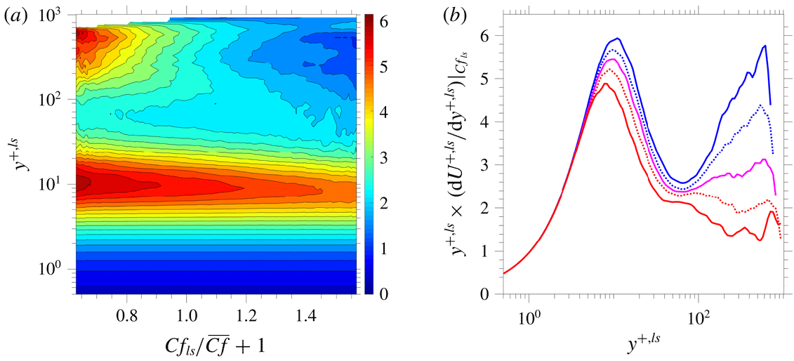
at which the production is high. This increase in production – and, to a lesser extent, the decrease at positive skin-friction fluctuations – are due to distortions in the mean velocity, which lead to a rise in shear strain in the outer region at negative fluctuations and a drop at positive fluctuations. This is confirmed by the map and profiles of the mean strain included in figure 8. As observed, the variations in the strain rate match closely those of the shear-production rate.
$y^{+,ls}\approx 300$
at which the production is high. This increase in production – and, to a lesser extent, the decrease at positive skin-friction fluctuations – are due to distortions in the mean velocity, which lead to a rise in shear strain in the outer region at negative fluctuations and a drop at positive fluctuations. This is confirmed by the map and profiles of the mean strain included in figure 8. As observed, the variations in the strain rate match closely those of the shear-production rate.

Figure 7. Conditional production rates of the total streamwise stress
 $\overline{uv}^{+,ls}(\text{d}U^{+,ls}/\text{d}y^{+,ls})$
premultiplied by
$\overline{uv}^{+,ls}(\text{d}U^{+,ls}/\text{d}y^{+,ls})$
premultiplied by
 $y^{+,ls}$
; (a) map (
$y^{+,ls}$
; (a) map (
 $y^{+,ls}$
–
$y^{+,ls}$
–
 $Cf_{ls}$
) and (b) wall-normal profiles for the values of
$Cf_{ls}$
) and (b) wall-normal profiles for the values of
 $u_{\unicode[STIX]{x1D70F},ls}$
identified in figure 3.
$u_{\unicode[STIX]{x1D70F},ls}$
identified in figure 3.

Figure 8. Conditional wall-normal derivative of the streamwise velocity
 $\text{d}U^{+,ls}/\text{d}y^{+,ls}$
premultiplied by
$\text{d}U^{+,ls}/\text{d}y^{+,ls}$
premultiplied by
 $y^{+,ls}$
; (a) map (
$y^{+,ls}$
; (a) map (
 $y^{+,ls}$
–
$y^{+,ls}$
–
 $Cf_{ls}$
) and (b) wall-normal profiles for the values of
$Cf_{ls}$
) and (b) wall-normal profiles for the values of
 $u_{\unicode[STIX]{x1D70F},ls}$
identified in figure 3.
$u_{\unicode[STIX]{x1D70F},ls}$
identified in figure 3.
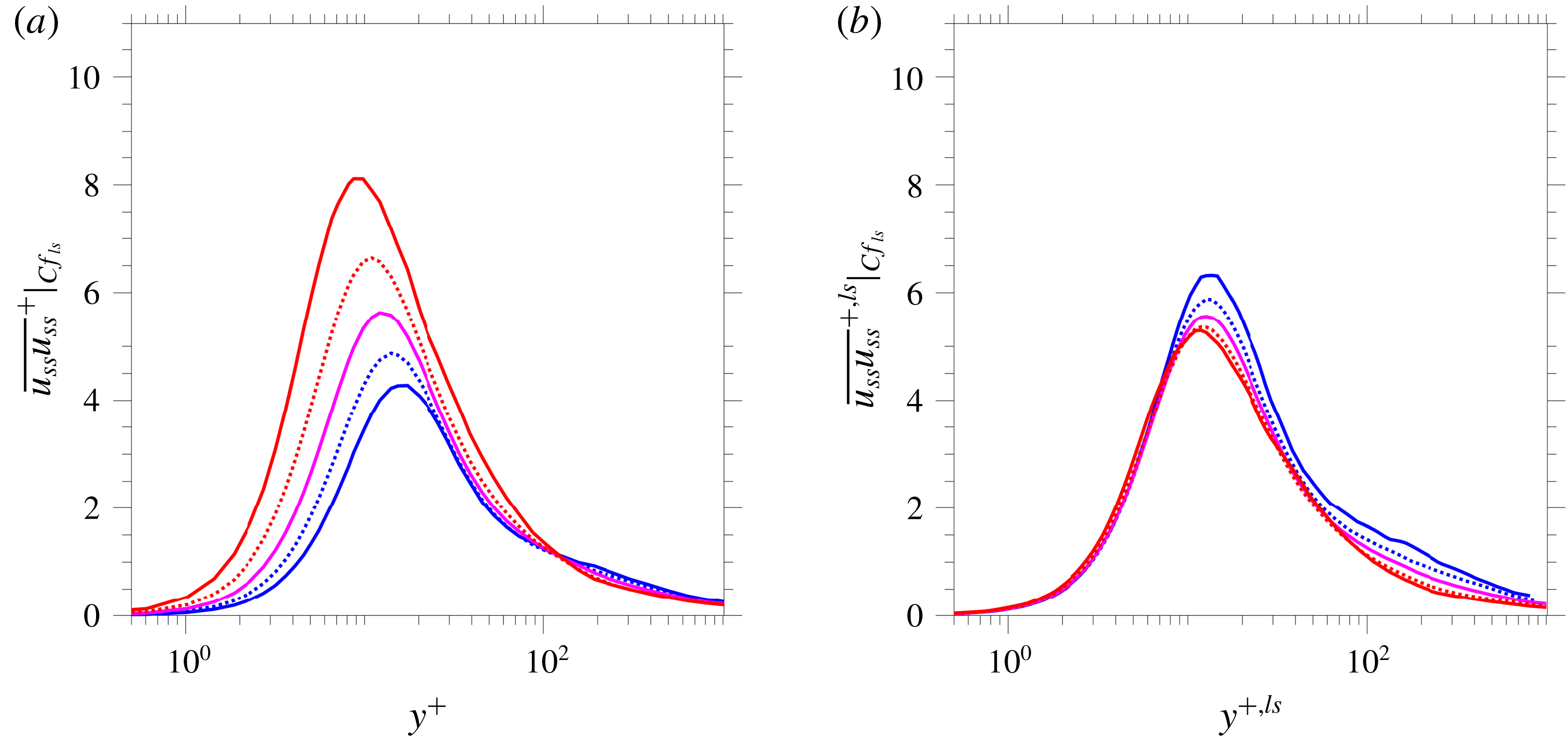
Significantly, the non-universal behaviour of the production rate extends, albeit weakly, towards the near-wall region down to
 $y^{+,ls}\approx 10$
, and the
$y^{+,ls}\approx 10$
, and the
 $\overline{u_{tt}u_{tt}}$
profiles in figures 4(a) and 4(b) show corresponding variations, including in the peak values of the streamwise stress. The question of whether the presence of the large-scale footprints in the viscous layer plays a direct role in this non-universal behaviour is answered by figures 9(a) and 9(b), which show profiles of the small-scale streamwise stress. Excluding the large-scale contributions is seen to substantially improve the collapse in the outer layer and to reduce the stress magnitude, as expected, but the discrepancies in the buffer layer persist and the trends are unchanged. This suggests that the lack of collapse in the streamwise total stress is due, as in the outer layer, to production of small-scale fluctuations, again by distortions in the locally scaled velocity profile. Indeed, reference to the strain-rate plots in figure 8 confirms that variations in the strain rate in the buffer match features in production rate and the streamwise stresses. Hence, the large-scale motions and the associated large-scale sweeps and ejections, which cause the velocity distortions, adversely affect the universality of the statistics close to the wall.
$\overline{u_{tt}u_{tt}}$
profiles in figures 4(a) and 4(b) show corresponding variations, including in the peak values of the streamwise stress. The question of whether the presence of the large-scale footprints in the viscous layer plays a direct role in this non-universal behaviour is answered by figures 9(a) and 9(b), which show profiles of the small-scale streamwise stress. Excluding the large-scale contributions is seen to substantially improve the collapse in the outer layer and to reduce the stress magnitude, as expected, but the discrepancies in the buffer layer persist and the trends are unchanged. This suggests that the lack of collapse in the streamwise total stress is due, as in the outer layer, to production of small-scale fluctuations, again by distortions in the locally scaled velocity profile. Indeed, reference to the strain-rate plots in figure 8 confirms that variations in the strain rate in the buffer match features in production rate and the streamwise stresses. Hence, the large-scale motions and the associated large-scale sweeps and ejections, which cause the velocity distortions, adversely affect the universality of the statistics close to the wall.


4 Conclusions
Although the QS concept and the related theory of Zhang & Chernyshenko are concerned with the universality of near-wall turbulence in the sense of its independence from the Reynolds number, this study focuses on the corollary – or an equivalent requirement – that the statistics for one Reynolds number should be invariant (universal) when these statistics are conditioned on the level of the large-scale skin friction that arises from the footprints of the large-scale outer motions. On the basis of this supposition, the available DNS-derived fields, including skin friction, have been subjected to a scale-separation method that allows the impact of the large scales on the small scales to be quantified and the fields to be scaled with the large-scale skin-friction footprints. The results included herein are thus in the form of skin-friction conditioned maps and profiles for the second moments and the production of the streamwise component.
The results show that the QS assumption, when pertaining to the total fluctuations, is confined to a thin layer – in the present case,
 $y^{+}<70{-}80$
. This is broadly in line with the limitation proposed by Zhang & Chernyshenko for their theory. Beyond this modest value, drastic departures from universality arise because the processes associated with the generation of the large scales do not scale with the local wall friction.
$y^{+}<70{-}80$
. This is broadly in line with the limitation proposed by Zhang & Chernyshenko for their theory. Beyond this modest value, drastic departures from universality arise because the processes associated with the generation of the large scales do not scale with the local wall friction.
An influential process is an asymmetric variation of the shear-induced production for positive and negative large-scale skin friction. This is due to wall-normal distortions in the large-scale strain rate, presumably provoked by large-scale ejections and sweeps. These distortions lead to a significant rise in the production of the outer structures for negative large-scale skin-friction fluctuations and, to a lesser extent, a decline for positive values.
The above distortions are observed to also have an impact on the small-scale turbulence right down to the viscosity-affected sublayer, adversely affecting the fidelity of the QS concept throughout the boundary layer. One aspect of this lack of fidelity is that the spanwise second moment scales especially poorly with the local wall shear, and this is attributed, with some confidence, to the role of splatting and anti-splatting associated with large-scale sweeps and ejections, respectively.
Acknowledgements
The research reported in this paper was undertaken within the framework of the EU–China project DRAGY, Grant Agreement 690623. The authors acknowledge the provision of HPC resources by the UK supercomputing facility ARCHER via the UK Turbulence Consortium funded by the EPSRC grant no. EP/L000261/1 as well as the CX2 facility of Imperial College London.