1. Introduction
The Late Palaeozoic (Stephanian to Permian times) is one of the most important stages of volcanic activity in western Europe and the Tethys realm (Arthaud & Matte, Reference Arthaud and Matte1977; Stampfli et al. Reference Stampfli, Mosar, Marquer, Marchant, Baudin, Borel, Vauchez and Meissner1998; McCann et al. Reference McCann, Pascal, Timmermann, Krzywiec, Lopez-Gomez, Wetzel, Krawczyk, Rieke, Lamarche, Gee and Stephenson2006; Bourquin et al. Reference Bourquin, Durand, Diez, Broutin and Fiuteau2007). However, in the Iberian plate a complete palaeogeographical picture of the setting of active faults and volcanic sources is not available yet because of the scarcity of outcrops and the difficulty of interpreting some of them owing to post-basinal compressional stages.
In the Pyrenean range, the Stephanian–Permian units occur as discontinuous outcrops of volcanic and continental deposits showing important thickness variations. These rocks were deposited in small and variably spaced intra-mountainous basins (J. Gisbert, unpub. Ph.D. thesis, Univ. Zaragoza, 1981; Aso et al. unpub. technical report, Instituto Geológico y Minero de España, 1987; B. Valero-Garcés, unpub. Ph.D. thesis, Univ. Zaragoza, 1991; Fig. 1a), where sedimentation was strongly controlled by the activity of faulted margins and volcanism played an important role (Martí & Mitjavila, Reference Martí and Mitjavila1987, Reference Martí and Mitjavila1988). Several studies deal with the geometry and dynamics of these basins and speculate on the causes of their origin (Soula, Lucas & Bessiere, Reference Soula, Lucas and Bessiere1979; J. Gisbert, unpub. Ph.D. thesis, Univ. Zaragoza, 1981; Bixel & Lucas, Reference Bixel and Lucas1983; Speksnijder, Reference Speksnijder1985). Nonetheless, this topic is still controversial and different geodynamic scenarios are evoked by the different authors: the basins are interpreted to be related to regional transtension or transpression (Soula, Lucas & Bessiere, Reference Soula, Lucas and Bessiere1979; Gisbert, Reference Gisbert and Comba1984; Lago et al. Reference Lago, Arranz, Pocoví, Galé, Gil-Imaz, Wilson, Neumann, Davies, Timmerman, Heeremans and Larsen2004; Román-Berdiel et al. Reference Román-Berdiel, Casas, Oliva-Urcia, Pueyo and Rillo2004; Cantarelli et al. Reference Cantarelli, Casas-Sainz, Corrado, Gisbert-Aguilar, Invernizzi and Aldega2009, in press; Rodríguez, Cuevas & Tubía, Reference Rodríguez, Cuevas and Tubía2012), to extension (Saura & Teixell, Reference Saura and Teixell2006) or to both regimes (Arthaud & Matte, Reference Arthaud and Matte1977; Ziegler, Reference Ziegler1988; Stampfli et al. Reference Stampfli, Mosar, Marquer, Marchant, Baudin, Borel, Vauchez and Meissner1998). There are also some open questions regarding the geometry and dynamics of the Stephanian, volcanic-dominated basins (Bixel & Lucas, Reference Bixel and Lucas1983; Martí & Mitjavila, Reference Martí and Mitjavila1987, Reference Martí and Mitjavila1988; Lago et al. Reference Lago, Arranz, Pocoví, Galé, Gil-Imaz, Wilson, Neumann, Davies, Timmerman, Heeremans and Larsen2004), where the massive nature of most of the volcanic and pyroclastic rocks makes difficult the determination of their internal structure and the recognition of flow directions, especially at the mesoscale.
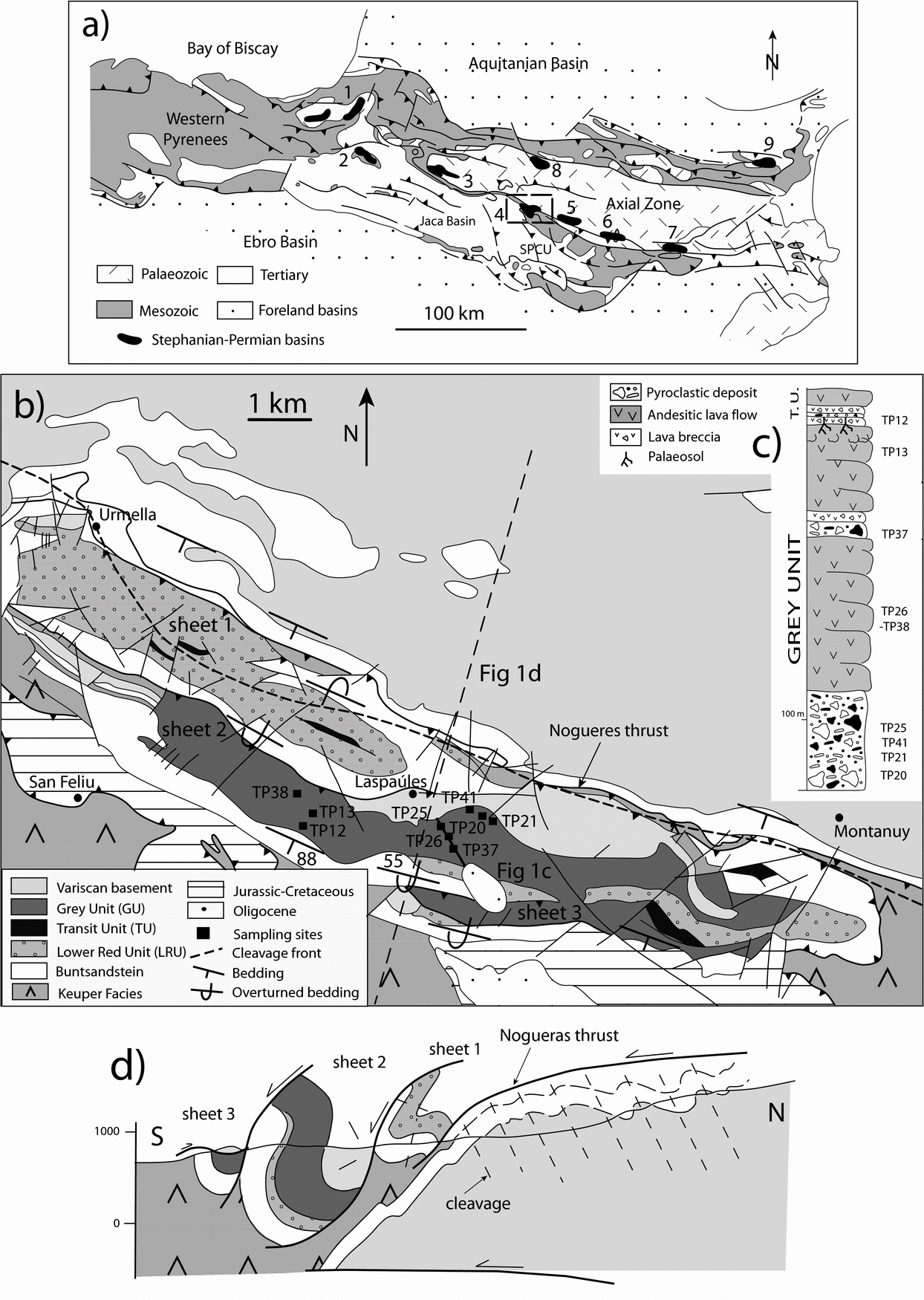
Figure 1. (a) Geological sketch of the Pyrenees showing location of the Stephanian–Permian basins (modified from Teixell, Reference Teixell1996); 1 – Basque basin, 2 – Pamplona basin, 3 – Aragón-Béarn basin, 4 – Castejón-Laspaúles basin, 5 – Malpàs-Sort basin, 6 – Cadí basin, 7 – Castellar-Camprodón basin, 8 – Central French basin, 9 – Eastern French basin (after J. Gisbert, unpub. Ph.D. thesis, Univ. Zaragoza, 1981). (b) Detailed geological map of the study area (modified from Aso et al. unpub. technical report, Instituto Geológico y Minero de España, 1987) including location of the sampling sites. (c) Stratigraphic log across the central part of thrust sheet 2 (Grey Unit), based on the description of Aso et al. (unpub. technical report, Instituto Geológico y Minero de España, 1987). (d) Geological cross-section (modified from Séguret, Reference Séguret1972). The location of the cross-section and the stratigraphic log is indicated in (b).
In this work we use the anisotropy of the magnetic susceptibility (AMS) and palaeomagnetic methods as a source of information to reconstruct and to better constrain the tectonic setting and internal geometry of the volcanic rocks in the Castejón-Laspaúles Stephanian basin (Fig. 1). On the one hand, AMS studies on lava flows and pyroclastic rocks (ignimbrites, pyroclastic surge deposits) have shown that their magnetic fabric is indicative of flow patterns and are therefore useful to locate the possible source areas (Ellwood, Reference Ellwood1978; Incoronato et al. Reference Incoronato, Addison, Tarling and Pescatore1983; Knight et al. Reference Knight, Walker, Ellwood and Diehl1986; Cañón-Tapia, Walker & Herrero-Bervera, Reference Cañón-Tapia, Walker and Herrero-Bervera1996; Cagnoli & Tarling, Reference Cagnoli and Tarling1997; Paquereau-Lebti et al. Reference Paquereau-Lebti, Fornari, Roperch, Thouret and Macedo2008; MacDonald et al. Reference MacDonald, Palmer, Deino and Shen2012). On the other hand, palaeomagnetic techniques are consolidated as a powerful tool to detect vertical axis rotations (VARs) (Allerton, Reference Allerton1998; Pueyo, Millán & Pocoví, Reference Pueyo, Millán and Pocoví2002; Platt et al. Reference Platt, Allerton, Kirker, Mandeville, Mayfield, Platzman and Rimi2003; Pueyo et al. Reference Pueyo, Pocoví, Millán, Sussman, Sussman and Weil2004; Weil & Sussman, Reference Weil, Sussman, Sussman and Weil2004; Oliva-Urcia & Pueyo, Reference Oliva-Urcia and Pueyo2007; Sussman et al. Reference Sussman, Pueyo, Chase, Mitra and Weil2012) and therefore accurately reconstruct the actual orientation of palaeoflow directions in absolute and relative frames.
The Castejón-Laspaúles basin is an a priori interesting basin to apply palaeomagnetic and rock magnetic analyses to because of (i) the varied nature of its filling (pyroclastic, sedimentary and lava flows), (ii) the thickness of the volcanic sequence, reaching 500 m in depocentral areas and (iii) the complex, post-basinal structure acquired during Tertiary times that makes difficult its reconstruction by means of conventional techniques.
2. Geological setting
The Castejón-Laspaúles basin belongs to the Nogueres Zone, located in the southern part of the Pyrenean Axial Zone, and limited to the south by the Jurassic, Cretaceous and Tertiary rocks of the South Pyrenean Central Unit (SPCU) (Fig. 1a). In this sector of the Pyrenean range, Stephanian–Permian units occur as discontinuous outcrops unconformably overlying the Variscan units of the Axial Zone (Gisbert, Reference Gisbert and Martínez Díaz1983; Gisbert, Martí & Gascón, Reference Gisbert, Martí and Gascón1985) (Fig. 1a).
The Castejón-Laspaúles basin has an ~ 800 m preserved thickness of syn-rift sedimentary and volcanic rocks (Valero-Garcés & Gisbert-Aguilar, Reference Valero-Garcés, Gisbert-Aguilar and Vera2004) and extends for ~ 17 km along strike (WNW–ESE direction) (Fig. 1b). Following Gisbert (unpub. Ph.D. thesis, Univ. Zaragoza, 1981), the Stephanian–Permian succession in this sector of the Pyrenees is divided in three units: (1) the ‘grey unit’, GU (Stephanian age), (2) the ‘transit unit’, TU (Stephanian–Autunian) and (3) the ‘lower red unit’ (LRU) (Autunian–Saxonian). The GU is more than 500 m thick and is constituted by pyroclastic deposits and dark-coloured lava flows of basaltic andesites (Aso et al. unpub. technical report, Instituto Geológico y Minero de España, 1987; García Senz et al. Reference García Senz, Ramirez Merino, Navarro Juli, Rodríguez Santisteban, Castaño, Leyva, García Sansegundo and Ramirez del Pozo2009a ,Reference García Senz, Ramirez Merino, Navarro Juli, Rodríguez Santisteban, Castaño, Leyva, García Sansegundo and Ramirez del Pozo b ) (Fig. 1c). The TU appears only as discontinuous outcrops of reduced thickness, including fine-grained sandstones, lacustrine shales, coal layers and pyroclastic rocks, that evolve laterally to fanglomerate deposits. In these deposits palaeocurrents are directed towards the south (García Senz et al. Reference García Senz, Ramirez Merino, Navarro Juli, Rodríguez Santisteban, Castaño, Leyva, García Sansegundo and Ramirez del Pozo2009b ). The LRU (also called the Peranera Formation; Nagtegaal, Reference Nagtegaal1969) is represented by more than 200 m of red shales and locally interbedded layers of sandstones and microconglomerates. This unit is unconformably covered by continental red beds, mainly sandstones, siltstones and shales, of Early to Middle Triassic age (Buntsandstein facies).
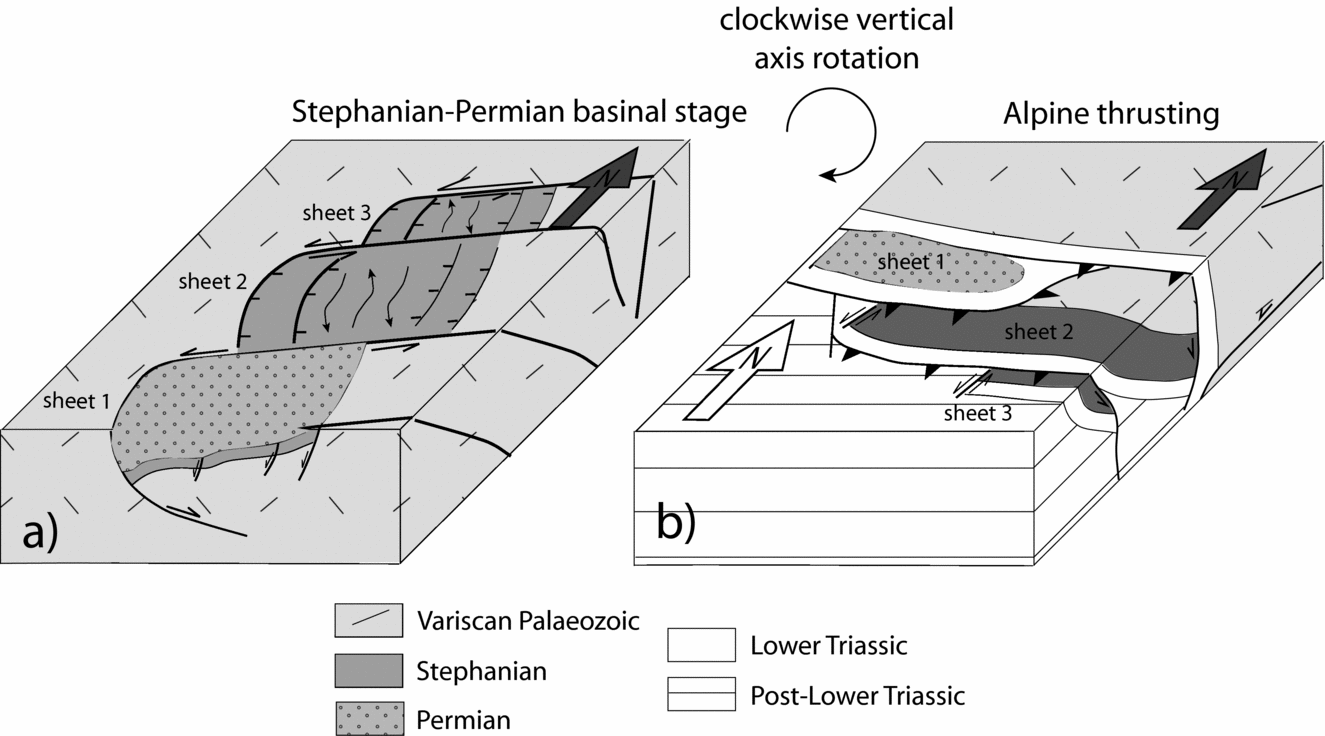
The Castejón-Laspaúles basin was inverted during the Pyrenean compression (Late Cretaceous to Tertiary times) and transported southwards within the Nogueres thrust sheet (Fig. 1b, d). In the study area, this main thrust is subdivided into three smaller-scale thrust sheets that are folded by underlying basement thrusts and involved in a foreland-dipping system at the front of an antiformal stack forming the Axial Zone. They are related to forelandward-rotated synformal anticlines (têtes plongeantes; Séguret, Reference Séguret1972). The northernmost thrust sheet (sheet 1 in Fig. 1b) contains mainly continental deposits from the LRU whereas the GU crops out within the central and southernmost thrust sheets (sheets 2 and 3 in Fig. 1b). In map view, the southern thrust sheets are shifted towards the east with respect to the thrust sheets located in a more northern position.
Thrusting was accompanied by the development of ESE–WNW-trending, S-verging folds, related to a pervasive cleavage affecting the Triassic and Palaeozoic units in the footwall of the Nogueres thrust and, partially, the Triassic and Permian rocks in the hangingwall (see the location of the cleavage front in Fig. 1b). The sampled volcanic and pyroclastic units are located South of the cleavage front and therefore not affected by macroscopic cleavage development.
3. Dynamics of the Stephanian–Permian basins in the Pyrenees
In spite of the controversy about the tectonic regime acting in the Pyrenees during Stephanian–Permian times, there is a general agreement on the influence of strike-slip faulting. Soula, Lucas & Bessiere (Reference Soula, Lucas and Bessiere1979) proposed that the development of the French Permian basins occurred during simple shear along previous basement faults of Variscan origin. The fault planes were subvertical, N 030° E- and N 070° E-striking, and the opening of the basins took place by block rotation under a general sinistral shearing (Fig. 2a). Bixel & Lucas (Reference Bixel and Lucas1983) described the western basins (Aragón-Bearn and Basque basins) as E–W and N–S half-grabens, whose opening was related to transcurrent shear. The basins were controlled by N–S-striking normal faults during the Stephanian, under a general dextral shear, and NE–SW-striking extensional faults during the Permian, under an overall sinistral wrench regime (Fig. 2b). Speksnijder (Reference Speksnijder1985) proposed for La Seu basin a simple shear mechanism along E–W-striking, dextral faults that generated E–W-oriented, strike-slip grabens, with alternating stages of transtension and transpression that were responsible for intrabasinal unconformities (Fig. 2c). Gisbert (unpub. Ph.D. thesis, Univ. Zaragoza, 1981) characterized also the activity of E–W-striking, sinistral transcurrent faults during the Stephanian and Early Permian, controlling the geometry of basins (Fig. 2d). Nonetheless, Saura & Teixell (Reference Saura and Teixell2006) interpreted the Stephanian–Permian basins located to the east of the study area (Erill Castell, Gramós and Estac basins) as extensional asymmetric grabens or half-grabens (Fig. 2e), controlled by normal E–W-striking faults acting as basin boundaries.
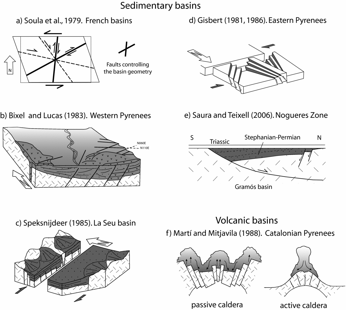
Figure 2. Different models proposed for the Stephanian–Permian basins in the Pyrenees (modified from Soula, Lucas & Bessiere, Reference Soula, Lucas and Bessiere1979; Bixel & Lucas, Reference Bixel and Lucas1983; Speksnijder, Reference Speksnijder1985; J. Gisbert, unpub. Ph.D. thesis, Univ. Zaragoza, 1981; Martí & Mitjavila, Reference Martí and Mitjavila1988; Saura & Teixell, Reference Saura and Teixell2006).
With regards to the volcanic basin activity, Martí & Mitjavila (Reference Martí and Mitjavila1987, Reference Martí and Mitjavila1988) proposed that the Malpàs-Sort, Cadí and Nevà-Campellas-Bruguera basins (eastern Pyrenees) behaved as passive volcanic calderas, with emissions of large volumes of magma and materials resulting from hydromagmatic processes. The geometry of these calderas was conditioned by the previous basin geometry, since the output of magma took place through the normal faults delimiting basin boundaries (Fig. 2f). On the other hand, the Castellar de N'Hug-Camprodón basin behaved as a sedimentary basin related to an active volcanic caldera on its western boundary (Fig. 2f). Towards the Western Pyrenees, the volcanic complexes show extrusive flows, but also important intrusive bodies. In the Anayet basin, volcanism is mainly represented by a thick laccolith that spreads laterally forming at least two sills, whereas in the Aragón–Subordán area a 35 m thick sill crops out (Lago et al. Reference Lago, Arranz, Pocoví, Galé, Gil-Imaz, Wilson, Neumann, Davies, Timmerman, Heeremans and Larsen2004).
4. Methodology
The samples used to analyse the magnetic fabrics and palaeomagnetism were directly drilled in the field with a gasoline-powered drill machine refrigerated with water. Nine sites, stratigraphically and areally distributed throughout the volcanic outcrops of the Castejón-Laspaúles basin, were collected. The samples belong to different kinds of pyroclastic units and andesitic lava flows and are located in thrust sheet 2 (see Fig. 1b), where the whole stratigraphic sequence is overturned (Fig. 1d). Between 12 and 21 cores were drilled in each sampling site, distributed in ~ 5 to 50 m of stratigraphic succession, and avoiding sampling close to the base or the top of the volcanic flows or ignimbritic sequences. The samples were oriented using a magnetic compass. Bedding/flow plane data were measured in the field for every sampling site. In site TP37, a conglomerate test was performed.
4.a. Magnetic mineralogy
In order to determine the magnetic mineralogy, three different analyses were performed: (1) temperature-dependent susceptibility curves, (2) isothermal remanent magnetization (IRM) and backfield acquisition curves (Dunlop, Reference Dunlop1972), and (3) stepwise thermal demagnetization of composite IRM (Lowrie, Reference Lowrie1990).
Temperature-dependent susceptibility curves between −195 and 700 °C were carried out in nine selected samples (one sample per site). At high temperatures, the variation of susceptibility with temperature allows the identification of magnetic phases based on their Curie (T c) or Néel temperature (T N) that defines the transition from ferromagnetic or antiferromagnetic to paramagnetic behaviours. This transition temperature is different for different ferromagnetic (sensu lato) minerals. At low temperatures, the mineral identification is based on slope variations related to changes in the crystallographic structure of the mineral (e.g. Verwey transition in magnetite at −152 °C; Verwey, Reference Verwey1939).
A KLY-3 Kappabridge combined with a CS-3 furnace (temperature range between 40 and 700 °C) and a CLS apparatus (temperature range between −195° and 0 ºC) (AGICO Inc., Czech Republic) was used for the temperature-dependent magnetic susceptibility (K–T) curves. Heating/cooling rates range between 11 and 14 °C min−1, respectively. The curves above room temperature were performed in an argon atmosphere in order to avoid mineral oxidations. Curie temperatures were determined following the method of Petrovský & Kapička (Reference Petrovský and Kapička2006).
To determine the carriers of the palaeomagnetic components, IRM and backfield acquisition curves, combined with thermal demagnetization of composite IRM, were conducted using a pulse magnetizer (maximum field of 2.5 T). The IRM acquisition curves were analysed by means of the IRM-CLG 1.0 worksheet (Kruiver, Dekkers & Heslop, Reference Kruiver, Dekkers and Heslop2001) that allows the quantification of the magnetic coercivity and the relative contribution to the IRM of the different components. Four samples (from four different sampling sites) were selected to carry out the IRM acquisition curves. They belong to different lithological types and cover the whole range of natural remanent magnetization (NRM) values and unblocking temperatures. Thermal demagnetization of composite IRM was performed in one sample per site. Three different, decreasing magnetic fields (1.5, 0.4 and 0.12 T) were applied along the three axes of the standard samples.
4.b. Magnetic fabrics at room and low temperatures
The magnetic susceptibility (K) of a rock is the ratio of induced magnetization (M) to an applied magnetic field (H): M = K·H. This physical property is described by a second-rank tensor and represented by an ellipsoid, which is defined by its three principal axes: maximum (K1), intermediate (K2) and minimum (K3). The orientation of the ellipsoid is mostly dependent on the crystallographic preferred orientation or the shape of the magnetic carriers.
In undeformed lavas, and away from the end of the flow, the mean magnetic foliation (perpendicular to the minimum axis) usually lies close to the flow plane, and the maximum susceptibility axis can be parallel (flow emplaced on significant slope) or perpendicular (flow emplaced on very weak slope) to the flow direction (Khan, Reference Khan1962; Halvorsen, Reference Halvorsen1974; Ellwood, Reference Ellwood1978; Cañón-Tapia, Walker & Herrero-Bervera, Reference Cañón-Tapia, Walker and Herrero-Bervera1996; Henry, Plenier & Camps, Reference Henry, Plenier and Camps2003; Cañón-Tapia, Reference Cañón-Tapia, Martin-Hernandez, Luneburg, Aubourg and Jackson2004). The magnetic foliation can exhibit a small imbrication angle relative to the flow plane that is upflow dipping in the lower part of the flow or downflow dipping in its lower part (Cañón-Tapia, Walker & Herrero-Bervera, Reference Cañón-Tapia, Walker and Herrero-Bervera1996, Reference Cañón-Tapia, Walker and Herrero-Bervera1997). In pyroclastic rocks, the direction of the Kmin axis is perpendicular to the bedding plane and the Kmax axis is commonly parallel to the flow direction (Knight et al. Reference Knight, Walker, Ellwood and Diehl1986; MacDonald & Palmer, Reference MacDonald and Palmer1990; Paquereau-Lebti et al. Reference Paquereau-Lebti, Fornari, Roperch, Thouret and Macedo2008), but flows perpendicular to Kmax axis directions have also been reported (Cagnoli & Tarling, Reference Cagnoli and Tarling1997). When Kmax is flow-parallel (and if there is no tectonic tilt at the site), the magnetic lineation coincides with the direction of maximum dip of the foliation plane. The slightly inclined foliation plane is usually interpreted to represent imbrication, and therefore the direction of maximum dip of the foliation plane can be used to determine flow directions.
The shape of the ellipsoid and degree of development of magnetic fabric are defined by means of two parameters: (1) the corrected anisotropy degree, Pj, and (2) the shape parameter, T, varying between T = −1 (prolate ellipsoids) and T = +1 (oblate ellipsoids). Pj and T are defined as (Jelinek, Reference Jelinek1981):
 \begin{equation*}
P_j \hspace*{-1.5pt}=\hspace*{-1.5pt} exp\sqrt {\{ 2[(\mu _1 \hspace*{-1.5pt}-\hspace*{-1.5pt} \mu _m )^2 \hspace*{-1.5pt}+\hspace*{-1.5pt} (\mu _2
\hspace*{-1.5pt}-\hspace*{-1.5pt} \mu _m )^2 \} \hspace*{-1.5pt}+\hspace*{-1.5pt} (\mu _3 \hspace*{-1.5pt}-\hspace*{-1.5pt} \mu _m )^2 ]\} }
\end{equation*
\begin{equation*}
P_j \hspace*{-1.5pt}=\hspace*{-1.5pt} exp\sqrt {\{ 2[(\mu _1 \hspace*{-1.5pt}-\hspace*{-1.5pt} \mu _m )^2 \hspace*{-1.5pt}+\hspace*{-1.5pt} (\mu _2
\hspace*{-1.5pt}-\hspace*{-1.5pt} \mu _m )^2 \} \hspace*{-1.5pt}+\hspace*{-1.5pt} (\mu _3 \hspace*{-1.5pt}-\hspace*{-1.5pt} \mu _m )^2 ]\} }
\end{equation*
 \begin{equation*}
T = \frac{{\left( {2\mu _2 - \mu _1 - \mu _3 } \right)}}{{\left( {\mu _1 - \mu _3 } \right)}}
\end{equation*}
\begin{equation*}
T = \frac{{\left( {2\mu _2 - \mu _1 - \mu _3 } \right)}}{{\left( {\mu _1 - \mu _3 } \right)}}
\end{equation*}
 $\mu _m = {{\left( {\mu _1 + \mu _2 + \mu _3 } \right)} \mathord{\left/ {\vphantom {{\left( {\mu _1 + \mu _2 + \mu _3 } \right)} 3}} \right. \kern-\nulldelimiterspace} 3}$
.
$\mu _m = {{\left( {\mu _1 + \mu _2 + \mu _3 } \right)} \mathord{\left/ {\vphantom {{\left( {\mu _1 + \mu _2 + \mu _3 } \right)} 3}} \right. \kern-\nulldelimiterspace} 3}$
.
The AMS at room temperature was measured in 141 standard rock samples (2.5 cm in diameter, 2.1 cm in height) with an average of 16 samples per site. The measurements were done with a KLY3S (AGICO Inc., Czech Republic) in the laboratory of the University of Zaragoza.
The analyses of low-temperature AMS (LT-AMS) were performed on samples from four selected sites, including pyroclastic deposits and lava flows. Samples were cooled down in liquid nitrogen (~ 77 K) for a minimum time of 30 minutes. The magnetic susceptibility was measured in air using the KLY3S, and the samples were cooled down again for ten minutes before the measurement in each new position (as in Lüneburg et al. Reference Lüneburg, Lampert, Hermann, Lebit, Hirt, Casey and Lowrie1999).
Low temperatures enhance the magnetic susceptibility of paramagnetic minerals, as established by the Curie–Weiss law (K = C/(T − T C), where K is the magnetic susceptibility, C is the Curie constant, T is the absolute temperature and T C is the Curie temperature). Assuming purely paramagnetic phases with a paramagnetic Curie temperature of around 0 K, the expected magnetic susceptibility is approximately 3.8 times higher at ~ 77 K (LT-AMS) than at room temperature.
4.c. Image analyses
Image analysis was performed in six samples from different sites. For each site, bi-dimensional orientation analyses were applied in thin-sections, which were taken from three perpendicular planes preferentially oriented with respect to the AMS ellipsoid axes: one plane is parallel to the magnetic foliation (perpendicular to K3) and the two remaining planes are perpendicular and contain K1 and K2 axes, respectively. In this way, the meaning of AMS in terms of mineral orientation can be better defined than with three randomly oriented perpendicular planes (Oliva-Urcia et al. Reference Oliva-Urcia, Casas, Ramón, Leiss, Mariani and Román-Berdiel2012 a; Izquierdo-Llavall et al. Reference Izquierdo-Llavall, Román-Berdiel, Casas, Oliva-Urcia, Gil-Peña, Soto and Jabaloy2012 b). The ImageJ public domain program (http://rsbweb.nih.gov/ij/index.html) was used to measure the shape preferred orientations (SPO) of the different components forming the volcanic and pyroclastic deposits (pyroclastic and lithic fragments, darker minerals, glass fragments, etc). The ImageJ software allows the approximation of the shapes of the fragments and individual mineral grains to ellipses and the measurement of the direction of their maximum axes. The determination of the SPO in three perpendicular planes has been used to reconstruct the bedding or flow plane, in order to compare it with the field data and the magnetic fabric results.
4.d. Palaeomagnetism
Both alternating field (AF) demagnetization and stepwise thermal demagnetization of the NRM were carried out at the Gams Palaeomagnetic Laboratory (Leoben University, Austria). Magnetization was measured using a 2G DC-SQUID magnetometer, and a MMTD-1 oven was used to thermally demagnetize the samples in steps ranging from 10 to 200 °C. AF demagnetization was performed by means of a 2G alternating field demagnetizer, in field steps ranging from 3 to 10 mT up to a maximum field of 120 mT. An average of 8–9 standard samples per site was measured. Palaeomagnetic components were fitted using the PCA method and site means were computed using Fisher (Reference Fisher1953) statistics. In both cases, the routine provided by the software Remasoft (Chadima & Hrouda, Reference Chadima and Hrouda2006) was used.
A ‘conglomerate test’ was performed at site TP37, where an ignimbritic sequence containing centimetric to decimetric-size, sub-angular andesitic lithic clasts crops out. The andesitic fragments probably derive from the underlying lava flows and were incorporated into the ignimbritic sequence during its deposition. In this site, samples from both the matrix and the andesitic lithic clasts were demagnetized.
5. Results
5.a. Field and petrographical data
All the sampling sites considered in this study belong to the GU (Fig. 1b), which shows massive andesites in the western and eastern basin margins (Aso et al. unpub. technical report, Instituto Geológico y Minero de España, 1987) and thick sequences of pyroclastic materials in the basin centre. The sampling sites are distributed within the central domain of the basin, where the following sequence is observed (Aso et al. unpub. technical report, Instituto Geológico y Minero de España, 1987; Fig. 1c): (1) a basal unit 130 m thick, constituted by breccias and thick ignimbritic sequences (sites TP20, TP21, TP25, TP38 and TP41), (2) 200 m of green andesites (TP26), (3) c. 20 m of ignimbrites and other pyroclastic deposits (TP37) and (4) c. 130 m of lava breccias and andesitic lava flows with an interbedded deposit of ignimbrites (TP12 and TP13). The top of the sequence is marked by the development of a thick palaeosol. Nonetheless, palaeosols are absent inside the GU, indicating that the deposition of the whole sequence was a relatively continuous and quick process. The pyroclastic units are mainly constituted by ignimbrites, but other types of deposits such as dome-breccias (to the bottom of the sequence) and pyroclastic surges with abundant contents of lithic fragments are also recognized (Aso et al. unpub. technical report, Instituto Geológico y Minero de España, 1987). Deposits are generally massive but flow or bedding planes could be measured in the field for all the sampling sites (Fig. 3a). Unfortunately, the determination of palaeoflow directions at the outcrop scale was not possible.

Figure 3. (a) Outcrop of ignimbritic deposits showing a well-defined bedding (site TP25). (b) Ignimbrite constituted by volcanic and lithic fragments embedded in a chloritic (Chl) matrix. Thin-section from site TP37 (crossed nicols). (c) Fine-grained andesitic lava flow mainly composed of plagioclase (Pl) and amphibole (Amp). Thin-section from site TP26 (crossed nicols). (d) Phenocrysts showing a preferred orientation. Thin-section from site TP38 (parallel nicols).
Nonetheless, the petrographical study reveals the presence of a well-developed flow orientation in most of the samples. The pyroclastic units are strongly heterometric, with highly vesicular volcanic fragments and quartz lithic fragments embedded in a fine-grained chloritic matrix (Fig. 3b). The lava flows show a finer and more homogeneous grain size (Fig. 3c). The main phenocrysts forming the sampled lithologies are plagioclase, opaque minerals, pyroxene, amphibole and, occasionally, olivine and chloritized biotite (Fig. 3c, d). The matrix is mainly composed by plagioclase, chlorite and opaque grains. Calcite cements are common in the pyroclastic rocks, filling in fractures and preferentially oriented vacuoles in vesicular volcanic fragments.
The outcrops of pyroclastic and volcanic deposits are limited to the west by NE–SW-striking faults in the central and southernmost thrust sheets (sheets 2 and 3 in Fig. 1b). The fault affecting the GU in the central thrust sheet (sheet 2) was interpreted as a syn-sedimentary normal fault, active during Stephanian times, since it is unconformably overlain by Triassic deposits (García Senz et al. Reference García Senz, Ramirez Merino, Navarro Juli, Rodríguez Santisteban, Castaño, Leyva, García Sansegundo and Ramirez del Pozo2009a ,Reference García Senz, Ramirez Merino, Navarro Juli, Rodríguez Santisteban, Castaño, Leyva, García Sansegundo and Ramirez del Pozo b ). This main structure could be syn-kinematic with a set of NNE–SSW- to NE–SW-striking listric normal faults, affecting the Devonian basement of the Nogueres Zone and the Stephanian volcanic rocks (M. P. Bates, unpub. Ph.D. thesis, Univ. Leeds, 1987). These faults strike N 020° E to N 055° E and dip both east and west.
5.b. Magnetic susceptibility and magnetic mineralogy
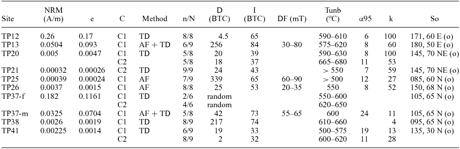
The sampled rocks show variable bulk magnetic susceptibility values, indicating a great heterogeneity in the mineralogical content of the volcanic and pyroclastic deposits, even in samples from the same site (see standard deviation in Table 1). Bulk magnetic susceptibility (K) ranges between 117 and 415·10−6 (SI), except in site TP12, where an anomalously high value of magnetic susceptibility was measured (1080·10−6) (Table 1).
Table 1. AMS data for the sampling sites in the Castejón-Laspaúles basin
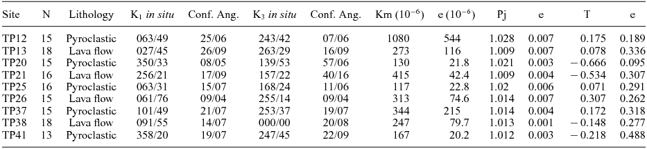
N – number of samples; K1 and K3 – mean (trend/plunge) of the magnetic lineation and of the pole of the magnetic foliation (Jelinek, Reference Jelinek1977) in geographic coordinates; Conf. Ang. – major and minor semi-axes of the 95 % confidence ellipse (Jelinek, Reference Jelinek1977); Km – magnitude of the magnetic susceptibility (·10−6); Pj – corrected anisotropy degree (Jelinek, Reference Jelinek1981); T – shape parameter (Jelinek, Reference Jelinek1981); e – standard deviation.
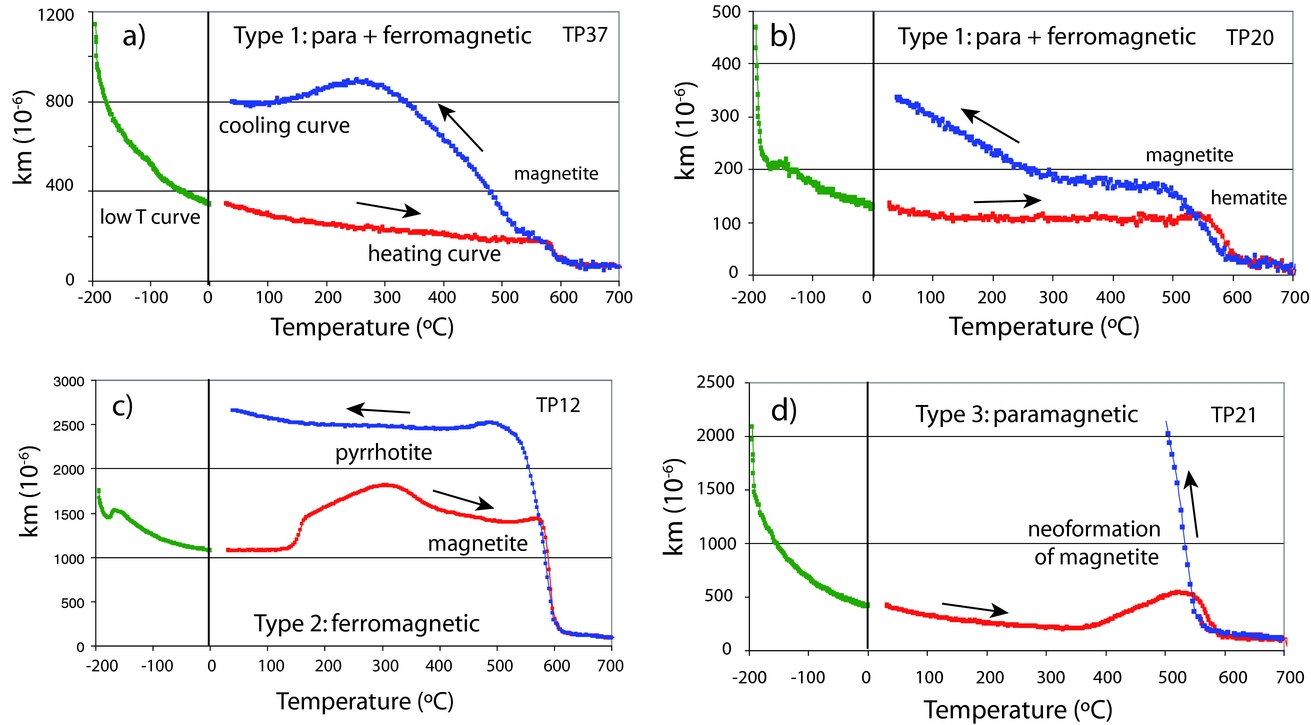
Temperature-dependent susceptibility measurements indicate, in seven out of nine samples, that magnetic fabrics are carried by a mixture of paramagnetic and ferromagnetic phases (type 1 curves in Fig. 4): they show a concave-hyperbolic shape at the beginning, indicating the contribution of paramagnetic carriers (iron-bearing silicates) and a drop in the magnetic susceptibility at c. 580 °C (T C of magnetite) (Fig. 4a). Only in two of these samples (TP20 and TP41) a second, weak phase was registered as indicated by a slight drop in susceptibility between 670° and 700 °C (TP20 is shown in Fig. 4b), suggesting the contribution of haematite in the ferromagnetic content (T N of haematite at 675 °C). The method of Hrouda (Reference Hrouda1994) allows the estimation of a heterogeneous paramagnetic contribution in type 1 curves, ranging between 50 % (sample TP20) and 93 %, and higher than 72 % when magnetite is the only ferromagnetic carrier. Temperature-dependent susceptibility measurements differ from type 1 curves in only two sites, TP12 (type 2, Fig. 4c) and TP21 (type 3, Fig. 4d). TP12 shows a purely ferromagnetic behaviour with generation of new ferromagnetic sensu lato phases while heating since magnetic susceptibility increases between 120 and 320 ºC and shows (i) a progressive drop between 320 °C (T C of ferromagnetic sensu lato iron sulphides) and 500 °C and a (ii) drop at c. 580 °C (T C of magnetite). On the other hand, TP21 shows a paramagnetic behaviour: the curve displays a concave-hyperbolic shape up to 360 °C, followed by an increase in the susceptibility between 360° and 530 °C and a drop between this temperature and 600 °C. This peak is most probably related to the neoformation of magnetite during heating due to oxidation of paramagnetic minerals (iron-bearing silicates such as pyroxene, amphibole, chlorite, biotite and olivine; see thin-sections in Fig. 3). K–T curves are very sensitive to mineral reactions, which occur during the heating if magnetic phases become unstable (e.g. Deng et al. Reference Deng, Zhu, Jackson, Verosub and Singer2001). In all the studied samples, the K–T curves are irreversible, probably owing to the mineralogical alteration of the samples during heating and the creation of new magnetite (Fig. 4).

Figure 4. Temperature-dependent susceptibility curves (−195 to 700 ºC) of four representative samples. Curves indicate (a, b) a mixed contribution of both paramagnetic and ferromagnetic carriers, (c) pure ferromagnetic behaviour and (d) prevalence of paramagnetic phases with neoformation of magnetite during heating.
The low-temperature curves describe a hyperbolic decay of susceptibility with increasing temperatures (Fig. 4). TP20 (Fig. 4b) and TP12 (Fig. 4c) show a slight increase in susceptibility at −165 °C, which could be related to a deviated Verwey transition of magnetite (Verwey, Reference Verwey1939).
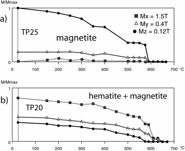
IRM acquisition curves were performed in four samples and show two different behaviours: (i) in samples TP37 and TP13 (Fig. 5a, b) a low coercivity carrier prevails, probably magnetite (mean coercivity ranges between 20 and 45 mT), which contributes 80–90 % to the IRM; (ii) in samples TP41 and TP20 a hard magnetic carrier dominates, probably haematite (mean coercivity ranges between 400 and 550 mT), which contributes 65 to 80 % to the IRM and prevents the complete saturation of the curves at 2.5 T (Fig. 5c, d). Thermal demagnetization of the composite IRM (Lowrie, Reference Lowrie1990) is consistent with the IRM acquisition curves. It shows that magnetite is the main ferromagnetic carrier, as evidenced by a sharp decay in the soft (120 mT) and intermediate (400 mT) components between 500 and 590 °C (Fig. 6a). In two of the sites (site TP20 in Fig. 6b and site TP41), an abrupt decay of the intermediate (400 mT) and hard axis (1500 mT) around 630–650 °C indicates the occurrence of haematite in the samples (Fig. 6b), consistent with the K–T curves that show a drop in susceptibility at around 680° C.
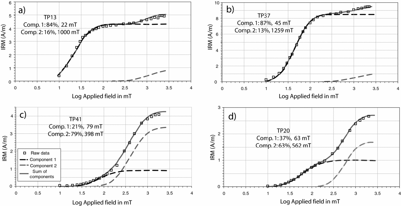
Figure 5. Analysis of the acquisition curves of the isothermal remanent magnetization (IRM) by means of the IRM-CLG 1.0 worksheet (Kruiver, Dekkers & Heslop, Reference Kruiver, Dekkers and Heslop2001).

Figure 6. Stepwise thermal demagnetization of the composite IRM (Lowrie, Reference Lowrie1990) in representative samples. Applied fields are 1.5, 0.4 and 0.12 T.
These results are consistent with the palaeomagnetic data and indicate that mainly magnetite and in some samples haematite are the main carriers of the palaeomagnetic components reported in the volcanic and pyroclastic units of the Castejón-Laspaúles basin.
5.c. Magnetic fabrics and image analysis
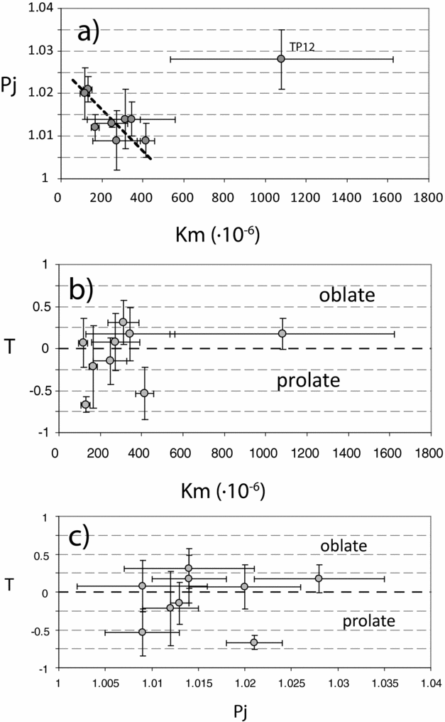
The Pj–Km (Fig. 7a) diagram shows (if site TP12 is not considered) a rough inverse correlation between them, with higher Pj values for the lower susceptibility samples. T–Km (Fig. 7b) and T–Pj (Fig. 7c) diagrams do not show a direct correlation between the shape parameter (T) and the bulk susceptibility (Km) or corrected anisotropy degree (Pj). These results suggest that Pj values could be controlled by the magnetic mineralogy content in the samples, while the T parameter seems to be independent of the lithology or magnetic mineralogy and can be interpreted in terms of the internal structure of the lava flows and pyroclastic deposits. The corrected anisotropy degree is rather low for the whole dataset, ranging between 1.009 and 1.028, with an average value of 1.016 (Table 1; Fig. 7a, b). No significant differences are observed between the lava flows and the pyroclastic samples. The shape parameter T shows a wide variability, from oblate to strongly prolate ellipsoids (Table 1; Fig. 7b, c). Negative T values are dominant in sites located close to the boundary with the Variscan basement, in the lower stratigraphic units; oblate ellipsoids (positive T values) are mainly concentrated in the intermediate and upper stratigraphic units.

Figure 7. (a) Corrected anisotropy degree (Pj) versus bulk magnetic susceptibility (Km). (b) Shape parameter (T) versus magnetic susceptibility (Km). (c) Shape parameter (T) versus the corrected anisotropy degree (Pj).
Concerning the orientation of the magnetic ellipsoid axes, sites can be grouped into two main types (AMS stereoplots are shown in Fig. 8). The first type (sites TP12, TP13, TP25, TP26 and TP37) shows an oblate to triaxial magnetic ellipsoid: the minimum susceptibility axes are perpendicular to the bedding or flow plane (or oblique in TP37) and the maximum and intermediate axes are weakly to well grouped within these planes. The second type (sites TP20, TP38 and TP41) refers to prolate AMS ellipsoids: the maximum axes are clearly clustered within the bedding or flow plane, and K3 and K2 axes describe a girdle perpendicular to K1. A different type of AMS ellipsoid was obtained in site TP21 that shows a prolate fabric, with well-grouped K1 axes perpendicular to bedding, and K2 and K3 scattered within the girdle corresponding to the bedding or flow plane. Jelinek's major semi-axes for the K1 95 % confidence ellipse (Jelinek, Reference Jelinek1977) are always smaller than 26°, and 67 % of the sites show angles lower than 20°, indicating a well-defined magnetic lineation for the whole studied area (Table 1).
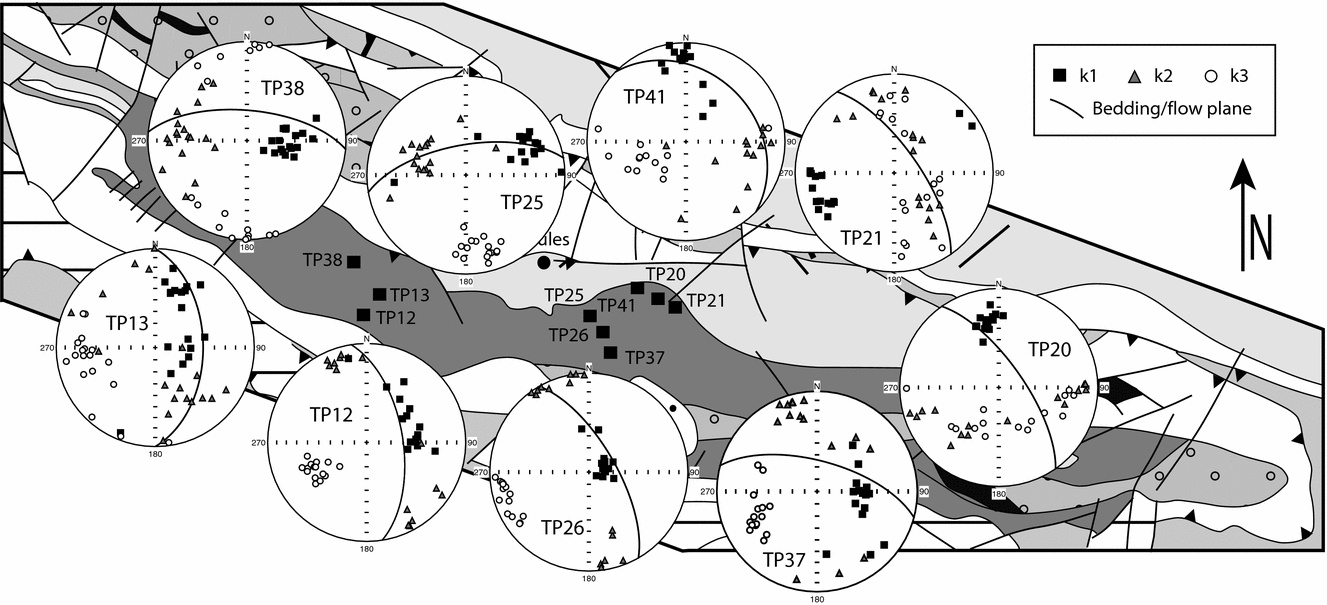
Figure 8. AMS ellipsoids obtained for each sampling site. The projection of the bedding/flow plane is shown.
The bulk susceptibility at low temperature (~ 77 K) is 1.7, 1.9, 2.1 and 2.9 times the bulk susceptibility at room temperature for the four selected sites (Fig. 9). These ratios (lower than the 3.8 expected for pure paramagnetic samples but higher than 1) could indicate a mixed contribution of ferromagnetic and paramagnetic phases to the AMS that is consistent with the results obtained in the temperature-dependent magnetic susceptibility curves. The orientation of the K1, K2 and K3 axes at low temperature (enhanced paramagnetic fabrics) overlaps the results of the AMS at room temperature (Fig. 9). Only in site TP26, slightly different results were obtained for the orientation of the AMS at room and at low temperatures (Fig. 9), suggesting a composite fabric: K1 and K2 axes are well grouped at room temperature, but at low temperature K1 shows a higher dispersion within the bedding plane and its average value is at an angle of ~ 35° with regards to the mean K1 at room temperature.
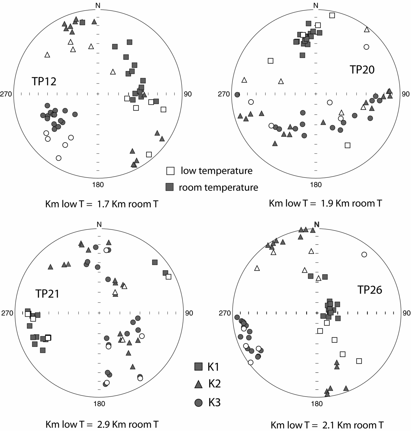
Figure 9. Stereoplot of AMS at room (grey symbols) and at low temperature (white symbols). See text for explanation.
The reliability of the AMS results was tested by means of image analysis. Results (Fig. 10) show that, in all the analysed samples, the AMS approximates the shape preferred orientation (SPO) measured for fragments and/or crystals. Therefore, the magnetic foliation plane can be relied upon as the bedding or flow plane, even in sites where this plane was not easily defined at the outcrop scale. The aspect ratio of a particle's fitted ellipse is always lower in the thin-sections parallel to the magnetic foliation and higher in the thin-sections perpendicular to it: eccentricity is either higher in the thin-section containing the K1 axis (Fig. 10a, TP13) or similar for both sections containing the K1 and K2 axes (Fig. 10a, TP25). In some of the samples, ImageJ reveals the existence of two preferred orientation maxima at lower angles (~ 20°), probably coinciding with one population of fragments whose longer axis is contained within the bedding or flow plane and a secondary population of imbricated particles (Fig. 10b, c, site TP25; for a discussion of this type of results see Oliva-Urcia et al. Reference Oliva-Urcia, Casas, Ramón, Leiss, Mariani and Román-Berdiel2012 a).

Figure 10. Image analysis results for the sections containing K1 and K3 axes (perpendicular to magnetic foliation and containing the magnetic lineation) in samples TP13 (to the left) and TP25 (to the right). (a) Original thin-section and after fitting the particle's shape to an ellipse by means of the ImageJ free software. (b) ImageJ results for the shape preferred orientation of the obtained ellipses. The histogram represents the number of ellipses versus the angle between their long axes and the reference line plotted in (a) (measured anticlockwise). (c) Comparison between the orientation of the AMS axis and the preferred shape orientation obtained by ImageJ in three perpendicular sections. AR is the aspect ratio of the ellipses fitted in each section (a higher value indicates a higher eccentricity).
5.d. Palaeomagnetism
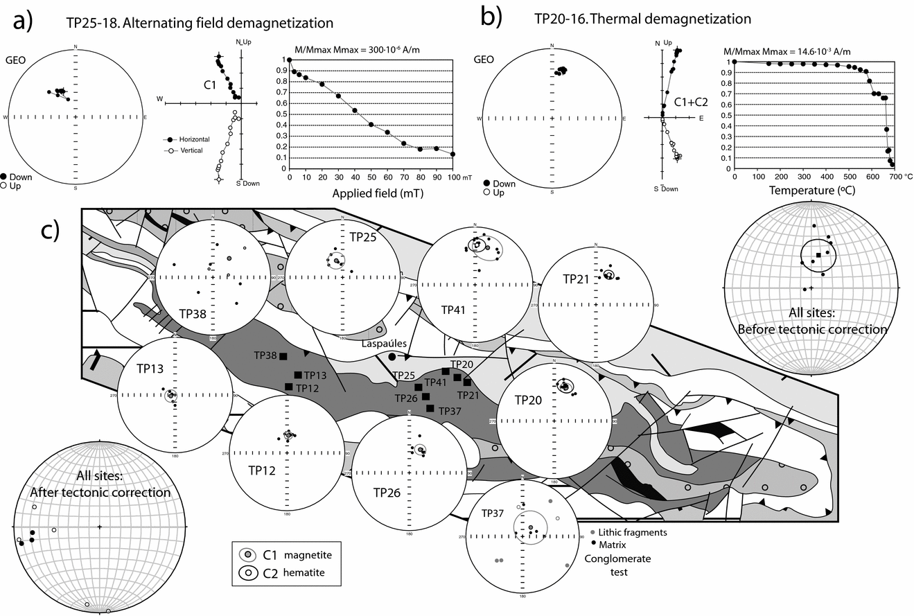
Stepwise thermal or AF demagnetization was performed in nine sampling sites (Table 2). AF demagnetization was successful (the remanent magnetization at 100–120 mT is lower than 20 % of the NRM) in pilot samples from four of the sites. Mean destructive fields vary in the different sites, and even among samples from the same site (Table 2): 32 % of the samples demagnetized by AF showed remanent magnetizations lower than 30 % of the NRM under fields of 40 mT and 68 % under fields of 70 mT (Fig. 11a). In samples that were thermally demagnetized (because AF was unable to fully destroy the remanence), two main temperature-related decays of magnetization could be distinguished (Fig. 11b): a lower temperature decay, between 550° and 630 °C, corresponding to magnetite/maghaemite (C1 in Fig. 11c), and a higher temperature decay, between 620° and 680 °C, corresponding to haematite (C2 in Fig. 11c). In sites where both minerals are present, no significant differences in the orientation of the components carried by them were observed (Table 2; Fig. 11b, c).
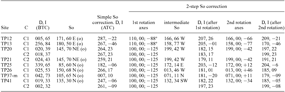
Table 2. Palaeomagnetic data for the sampling sites in the Castejón-Laspaúles basin

Site TP37 shows the conglomerate test (TP37-m refers to the matrix and TP37-f to the lithic fragments). NRM – natural remanent magnetization (in Ampere/metre); e – standard deviation of NRM; C – palaeomagnetic component (C1 for magnetite/maghaemite and C2 for haematite); demagnetization method (TD – thermal demagnetization; AF – alternating field demagnetization); n/N – number of samples used to calculate the mean from the total number of standard samples; D (BTC) and I (BTC) – declination and inclination before tectonic correction; DF – mean destructive field (the remanent magnetization is lower than 30 % of the NRM); Tunb – maximum unblocking temperature; α95 and k are the statistical parameters of a Fisherian distribution; So – bedding plane (strike and dip; o for overturned beds).

Figure 11. Results of the palaeomagnetic study. Orthogonal diagrams, decay of the magnetization and lower hemisphere equal-area stereographic projections during stepwise AF (a) or thermal (b) demagnetization. (c) Lower hemisphere stereoplots showing the samples’ components (calculated using the PCA method) and the site means (Fisher statistics; Fisher, Reference Fisher1953). The lateral stereoplots include the site means for the whole dataset before and after simple-bedding correction. In sites were both, components C1 and C2 were defined, the one showing the smaller α95 was chosen.
The demagnetization of the whole dataset reveals the presence of one stable, well-defined component in all but one of the sites (TP38) (Table 2). This component is N-trending and shows variable inclinations, from subhorizontal to subvertical. It displays a normal polarity direction in geographic coordinates and is scattered along a NNE–SSW-striking plane, perpendicular to the trend of the fold axes. This distribution strongly suggests a pre- or syn-folding acquisition (Table 2; Fig. 11c). The average orientation for this component (computed from the average values of each site) is Dec., Inc. = 012, 59 (α95 = 16°, k = 11) (Fig. 11c). After the simple bedding-plane restoration, this component is subhorizontal or shallowly plunging and can be subdivided into two groups (Fig. 11c): (1) two sites show S-trending and subhorizontal components and (2) 6 sites display W-trending components with shallow to intermediate inclinations. The distribution of this component after tectonic correction is strongly conditioned by the strike of the bedding or flow plane: W-trending components result from the simple restoration of N-S or NW-SE-striking bedding/flow planes and S-trending components from the restoration of E-W-striking bedding/flow planes.
In site TP37 it was possible to perform a conglomerate test (Watson, Reference Watson1956), which indicates that the palaeomagnetic component of the clasts (centimetric lithic fragments in the ignimbrite) has a random distribution (Fig. 11c) whereas that of the matrix shows a better grouped distribution. Samples containing both matrix and clasts also showed a random distribution and have been disregarded in Figure 11c. The result of the conglomerate test suggests a primary origin for the calculated palaeomagnetic components.
6. Discussion
6.a. Contribution of palaeomagnetic data to the restoration of bedding and the determination of vertical axis rotations
Two main arguments suggest that the palaeomagnetic component defined in the study area was acquired early with regards to Alpine compressional deformation: (i) the distribution of the components defined for the whole dataset (Fig. 11c) shows they are folded following the Alpine structure, and therefore, its acquisition pre-dates, or is early, with regards to the compressional stages and (ii) the conglomerate test is positive, indicating that the component was acquired very early in the history of the deposit and probably has a primary origin. After simple-bedding restoration (Figs 11c, 12) the palaeomagnetic components diverge into two different groups separated an angle of ~ 90°: sites where the bedding or flow plane was strongly oblique to the Alpine structures (N–S- to NW–SE-striking planes in sites TP12, TP13, TP20, TP21, TP26 and TP41) show a W-trending component after bedding restoration, and sites where the bedding/flow planes strike sub-parallel to the Alpine structure (E–W- to WNW–ESE-striking planes in sites TP25 and TP37) show a S-trending component. There is a clear influence of the strike of bedding on the restoration that cannot be justified in terms of vertical axis rotations (VARs) if palaeomagnetic studies in the adjacent Triassic red beds are taken into account (Bates, Reference Bates1989; Izquierdo-Llavall et al. Reference Izquierdo-Llavall, Casas, Oliva-Urcia and Scholger2012a ). Disregarding the possibility of relative VARs of almost 90° between the different sites, the existence of bedding/flow planes striking oblique to the main Pyrenean direction can be interpreted as due to a pre-compressional tilting of the beds. In this situation, a two-step bedding correction can be applied (Fig. 12; Table 3) according to the most plausible sequence of events: (1) restoration of the compressional structure and (2) tilt correction of the bedding/flow plane resulting after the first step. For the first step we used the orientation of bedding planes measured in the Lower Triassic red beds (Buntsandstein unit) that overlie the volcanic units sampled in the different sectors of the basin (see structural data in Fig. 1b and Table 3). The strike of bedding in the Lower Triassic units is subparallel to the fold axes and to the strike of thrusts, and its dip reflects the superimposition of horizontal axis rotations related to two coaxial compressional stages: the folding of the beds in hangingwall, thrust-related anticlines, and its foreland-wards tilting due to the emplacement of underlying basement thrusts (see cross-section in Fig. 1d). The surface obtained after this first step represents the orientation of the beds prior to the Alpine compression (Fig. 12a), and indicates that there was a dominant intermediate-to-steep westward tilting of the beds pre-dating Pyrenean folding (Table 3). After the two-step bedding correction, the palaeomagnetic components are well grouped and show a subhorizontal, SSW-trending direction (Dec., Inc. = 193, −05; α95 = 18°, k = 0.9). When compared to the Stephanian reference (Dec., Inc. = 336, −06; α95 = 12.5°; computed for a central position of the basin from three references in Van der Voo, Reference Van der Voo1969, compiled by Osete & Palencia, Reference Osete and Palencia-Ortas2006), they show similar inclination values but are clockwise rotated an average of +37° (Fig. 12b). The error in the rotation (α95 of the average component calculated from the new dataset +α95 of the Stephanian reference) is big (±32°) but the inferred mean clockwise rotation is statistically distinguishable from the Stephanian reference. Similar rotation values have been obtained in the overlying Triassic red beds (Izquierdo-Llavall et al. Reference Izquierdo-Llavall, Casas, Oliva-Urcia and Scholger2012a ) with regards to the Permian-Triassic reference for this sector of the Pyrenees (Dec., Inc. = 345, 14; α95 = 5.8°, k = 138.3; from data by Parés, van der Voo & Stamatakos, Reference Parés, van der Voo and Stamatakos1996; Schott & Perés, Reference Schott and Perés1987 and Osete et al. Reference Osete, Rey, Villalaín and Juárez1997, compiled in Osete & Palencia, Reference Osete and Palencia-Ortas2006). In all sites, a reverse polarity component is obtained (for both, northern and southern hemisphere positions), consistent with the Kiaman reverse superchron (312–262 Ma) (Molina-Garza, Geissman & van der Voo, Reference Molina-Garza, Geissman and van der Voo1989).
Table 3. Simple and two-step bedding restoration

For each component: orientation (declination, D and inclination, I) before tectonic correction (BTC), orientation after simple-bedding (So) correction (ATC), rotation axis used in the two-step bedding correction, orientation of the ‘intermediate bedding’ obtained after the first rotation and orientation of the palaeomagnetic component after the first and the second rotations.
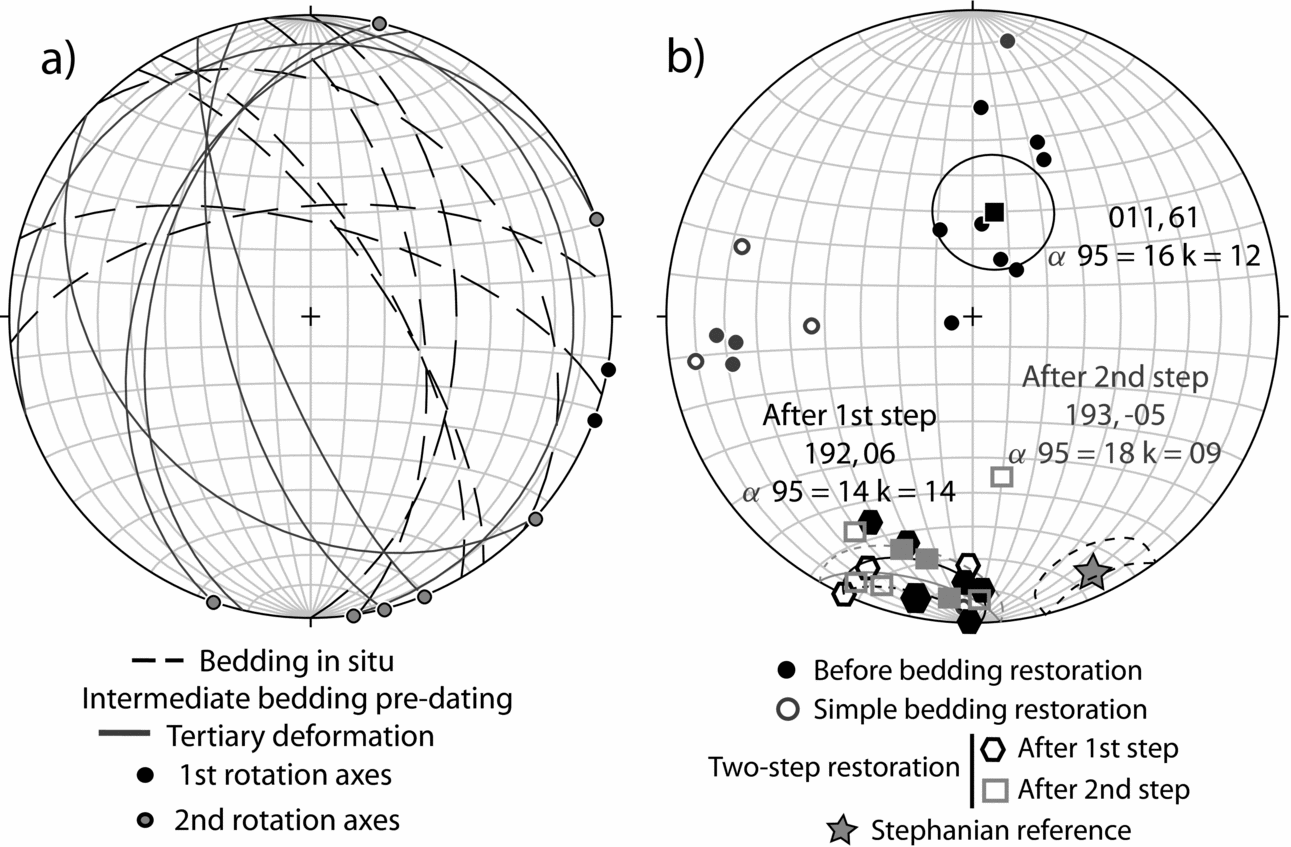
Figure 12. (a) Stereoplot showing bedding or flow planes before tectonic correction and after restoration of Alpine folding. (b) Orientation of the palaeomagnetic components before and after tectonic correction (using the two-step and the simple-bedding restoration). After the first step, a reverse polarity, southern hemisphere component is dominant and α95 is 14°. After the second step α95 is 18°; some sites keep a reverse polarity, southern hemisphere component while others show a reverse polarity, northern hemisphere component. The average component is clockwise rotated with regards to the Stephanian reference: Dec., Inc. = 336, −06; α95 = 14° (calculated from three references in Van der Voo (Reference Van der Voo1969) for a central position of the basin: latitude of 42° 28′ N and longitude of 0° 36′ E).
6.b. Interpretation of magnetic fabrics
The stereoplots in Figure 13a show the whole dataset of in situ magnetic fabrics. K1 axes are distributed within a girdle (170, 60 E) that is approximately perpendicular to the regional fold axis and contains two maxima: a N-trending, shallowly plunging maximum and an E-trending, steeply plunging maximum. K3 describes a principal, W-trending and intermediately plunging maximum and a secondary, S-trending, shallowly plunging maximum. K3 axes are mostly subperpendicular to the bedding or flow planes while K1 axes are contained within these planes (except in TP21), showing rakes that range between 90 and 25°, and are folded following the same pattern as the palaeomagnetic components.
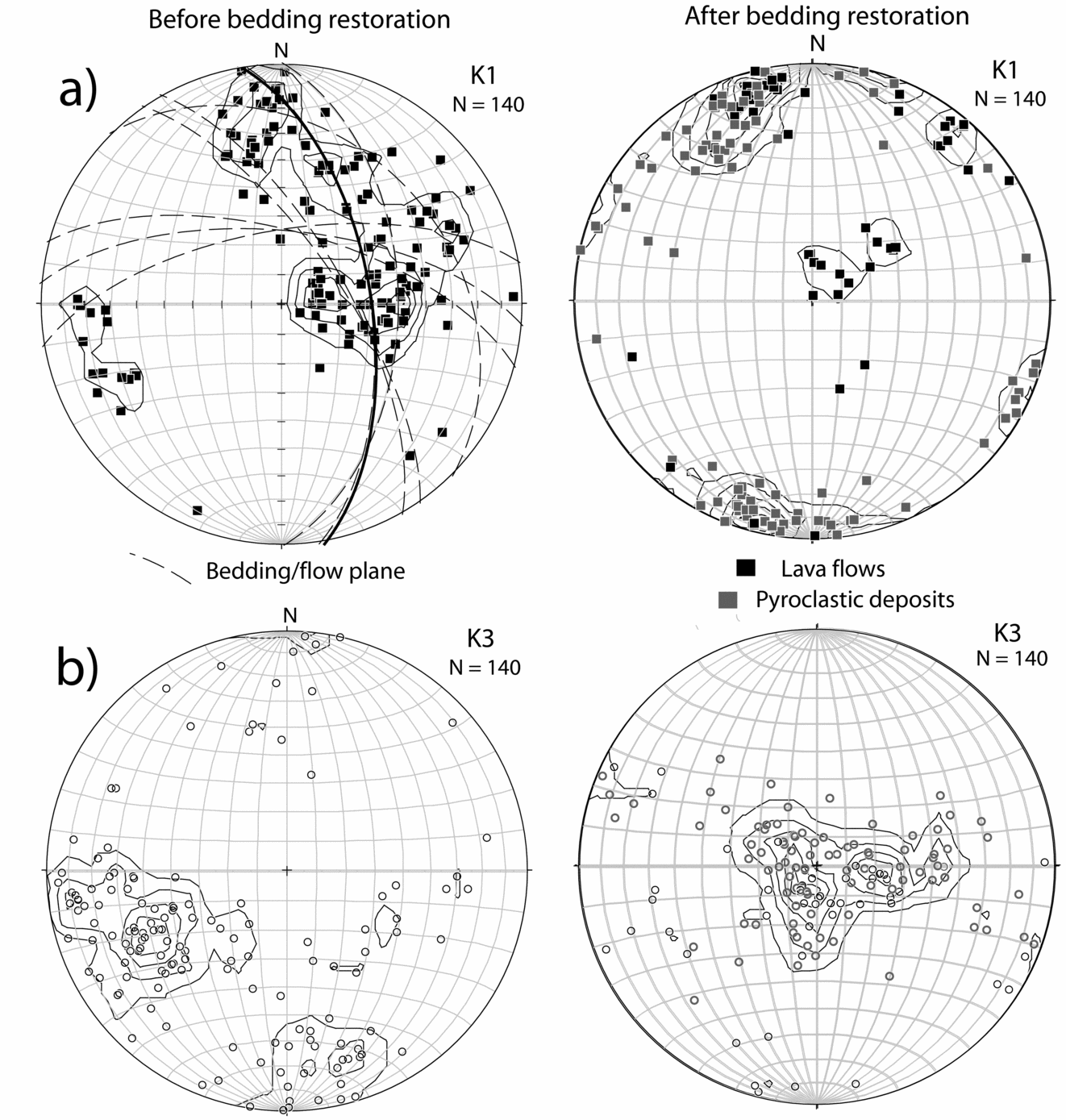
Figure 13. Stereoplots and density diagrams of K1 (a) and K3 (b) before and after bedding correction for all the measured samples.
After bedding correction (the two-step bedding correction previously described was applied), K3 and K1 axes become subvertical and subhorizontal, respectively (Fig. 13b) and show a better grouping. This distribution suggests that magnetic fabrics pre-date Pyrenean folding and register the volcanic or volcano-sedimentary fabric acquired during Stephanian times. A volcanic or volcano-sedimentary origin for the magnetic fabrics is also suggested by:
-
(i) Microstructural observations: thin-sections show flow evidences (such as oriented vacuoles and imbricated fragments) with an orientation that is consistent with the measured AMS; compression-related cleavage was not developed at the microscale.
-
(ii) Image analysis results that show a good correlation between the magnetic ellipsoid and the SPO of the different types of particles forming the lava flows and pyroclastic units.
A particular type of magnetic fabric has been obtained in site TP21, where K1 axes are almost perpendicular to the flow surface measured in the field. This kind of distribution could be expected: (i) in areas located close to the frontal boundary of the lava flows (Ellwood et al. Reference Ellwood, Osipov, Kafafy, Henry, Chlupakova, Tarling and Hrouda1993 and references therein) where particle rotation is a common process, or (ii) in the presence of single-domain magnetite causing an inverse fabric (Rochette, Reference Rochette1988; Potter & Stephenson, Reference Potter and Stephenson1988). In the remaining sites, K3 axes are subperpendicular to bedding, showing some dispersion (Fig. 13b), and no significant differences are observed between the orientation of K3 in pyroclastic units and lava flows. After bedding restoration, K1 axes are subhorizontal and show two preferred orientations, NNW–SSE and NNE–SSW.
In regional studies, magnetic lineations in ignimbritic deposits have usually been interpreted as parallel to flow directions (Knight et al. Reference Knight, Walker, Ellwood and Diehl1986; MacDonald & Palmer, Reference MacDonald and Palmer1990; Paquereau-Lebti, Reference Paquereau-Lebti, Fornari, Roperch, Thouret and Macedo2008), especially when constant trends are observed in different parts of the stratigraphic sequence and in the different levels forming one ignimbritic deposit. In our study area, K1 axes in both ignimbritic units and lava flows show a good agreement and a constant orientation in (i) the different rock types, (ii) the different stratigraphic levels of the ~ 500 m thick volcanic sequence and (iii) the different layers or flows sampled at every site. We consider that, in the absence of flow markers at the outcrop scale, this constant orientation can be interpreted in terms of flow-parallel K1 axes that would indicate an average ~ N–S-trending flow (NNW–SSE- and NNE–SSW dominant flow directions). The different lithological types (lava flows and pyroclastic units) show the same flow pattern, probably indicating a constant source area. With regards to K3 axes, there is a higher dispersion, but a N–S-elongated maximum can be observed in the stereoplot that shows the whole dataset (see Fig. 13b). This maximum indicates foliation planes that are slightly imbricated towards the N and S with respect to bedding/flow planes, which would be in agreement with a dominant flow in this direction.
The restoration of the clockwise VAR of +37° detected by palaeomagnetic data would convert the inferred, average ~ N–S-trending flow (in present-day coordinates) into a NW–SE-trending flow pattern during Stephanian times. With regards to the flow sense, no definitive indications are given by the magnetic fabric results.
Furthermore, AMS ellipsoids could be interpreted in terms of dominant flow mechanisms (Cagnoli & Tarling, Reference Cagnoli and Tarling1997): laminar flows are usually related to triaxial AMS ellipsoids (well defined in sites TP25 and TP26, to the base and intermediate part of the volcanic sequence, see Fig. 1c), while turbulent deposits are characterized by oblate ellipsoids with well-defined K3 axes and K1 and K2 axes distributed in a girdle (sites TP12, TP13 and TP37, ignimbrites and lava flows to the top of the volcanic sequence, see Fig. 1c).
6.c. Implications for the tectonic-controlled volcanism in the Castejón-Laspaúles basin
Field evidence and the new palaeomagnetic and magnetic fabric data shown in this work allow the inference of the following constraints with regards to the configuration of the Castejón-Laspaúles basin during Stephanian times:
-
(1) The comparison between the orientation of the obtained palaeomagnetic components and the Stephanian reference for the Iberian plate evidences an average clockwise rotation of +37° for the volcanic deposits. Similar rotations can be inferred from data in the overlying Triassic red beds (Bates, Reference Bates1989; Izquierdo-Llavall et al. Reference Izquierdo-Llavall, Casas, Oliva-Urcia and Scholger2012a ), indicating that the VAR took place mainly after Triassic times, probably owing to thrusting during the Pyrenean compressional stage (Fig. 14).

Figure 14. (a) Reconstruction of the basinal configuration during Stephanian–Permian times considering the magnetic fabrics and palaeomagnetic study. (b) Sketch showing the Alpine configuration of the Castejón-Laspaúles basin.
-
(2) Magnetic fabric results could be interpreted in terms of flow directions and would indicate a dominant N–S-trending flow direction (in present-day coordinates) for both lava flows and pyroclastic deposits. The expected flow pattern in a passive caldera (Martí & Mitjavila, Reference Martí and Mitjavila1987, Reference Martí and Mitjavila1988) completely surrounded by active extensional faulting would impose a concentric flow pattern. Nonetheless, the existence of a preferred N–S-trending flow pattern can only be explained in the context of (i) a passive caldera where only E–W-striking, straight and deep-rooted faults limiting the basin to the north and/or south are controlling magmatic emissions or (ii) an active caldera or volcanic building located north and/or south of the basin. There is no evidence of the presence of this sort of magmatic building and, therefore, we propose that the first option is the most plausible volcanic scenario. The existence of deep-rooted faults controlling magmatic emissions is consistent with the presence of granulitic xenoliths from the lower crust, detected by Arranz Yagüe, Galé-Bornao & Lago-San Jose (Reference Arranz Yagüe, Galé-Bornao and Lago-San Jose1998) in adjacent areas.
-
(3) The inferred westward tilting of bedding and/or flow planes can be explained by the existence of normal faults, N–S-striking (in present-day coordinates), that controlled the infill geometry and limited the basin to the west.
-
(4) The proposed, dominant fault strikes acting during Stephanian times can be recognized in the present-day structure (Fig. 1b). The E–W-striking, deep faults controlling the magmatic emissions could be later reactivated as thrust planes during Alpine thrusting (as suggested by Saura & Teixell, Reference Teixell1996 for adjacent Stephanian–Permian basins) while the N–S-striking normal faults could coincide with the oblique structures at the westward limits of thrust sheets (sheets 1, 2 and 3 in Fig. 1b; see comments at the end of section 5.a.), reactivated as strike-slip faults during Pyrenean compression (Fig. 14a, b).

In summary, a distinction can be made between deep-rooted E–W faults, probably responsible for magmatism, and shallow-rooted, listric faults of N–S orientation (both in present-day coordinates), controlling the early tilting of beds. According to these inferred fault patterns, and considering the present-day architecture of the Nogueres Zone (in map view, the southern thrust sheets are shifted towards the east with respect to the thrust sheets located in a more northern position) the Stephanian–Permian basins can be envisaged as rhomb-shaped troughs between left-lateral strike-slip faults with extensional ends located to the west and eastward shifted for the more northern positions (Fig. 14a). This model is consistent with the basin geometry and the tectonic regime proposed by Soula, Lucas & Bessiere (Reference Soula, Lucas and Bessiere1979) for the French Permian basins, Bixel & Lucas (Reference Bixel and Lucas1983) for the Western Pyrenees and Gisbert (unpub. Ph.D. thesis, Univ. Zaragoza, 1981) for the Eastern Pyrenees. It differs in the sense of shear from the model of Speksnijder (Reference Speksnijder1985) for La Seu basin and in the regional tectonic regime and the role of the E–W-striking faults from the basin model proposed by Saura & Teixell (Reference Saura and Teixell2006).
7. Conclusions
The magnetic fabrics and palaeomagnetism dataset presented in this work led to the following conclusions:
-
(i) AMS ellipsoids show K3 axes that are usually perpendicular to bedding or flow planes and K1 is generally well grouped within these planes (Table 1). Image analysis evidences that magnetic fabrics approximate the SPO of the fragments and minerals forming the different lithological units (Fig. 10).
-
(ii) Flow planes are in several sites oblique to the Alpine structure and this distribution is interpreted as being due to a westward tilting of the beds pre-dating compression.
-
(iii) The palaeomagnetic study (Figs 11, 12) reveals the presence of one stable primary component clockwise rotated an average of +37° (±32°).
-
(iv) Magnetic fabrics are interpreted as being acquired during the emplacement or deposition of the volcanic and pyroclastic units and indicate a preferred N–S-trending flow direction (Fig. 13) in present-day coordinates. Both pyroclastic and volcanic units probably shared the same source area.
-
(v) Emissions were probably related to E–W-striking, deep-rooted faults limiting the basins. These faults were coeval to the development of N–S-striking normal faults limiting the basins preferentially towards their western ends. The existence of these two fault sets and the distribution of basins are consistent with a sinistral shear regime during the development of the Castejón-Laspaúles basin (Fig. 14).
Acknowledgements
The authors thank Cristina García and Teresa Román for her help during field and laboratory work and Manuel Tricas for the preparation of thin-sections. This work forms part of the research projects CGL2009-08969 and CGL2006-05817 (Spanish Ministry of Education) and is included in the objectives of the pre-doctoral grant AP-2009-0554 (Esther Izquierdo) (Programa de formación de profesorado universitario, Spanish Ministry of Education). Funding from the Instituto de Estudios Altoaragoneses is also acknowledged. BOU acknowledges the JAEDOC postdoctoral programme financed with ESF. The authors acknowledge the careful and constructive revisions by B. Henry and an anonymous reviewer.