


1 Introduction
Plumes are convective flows with predominantly vertical motion, which occur whenever buoyant fluid is persistently released from a localised source. Such flows are common in a wide variety of natural and industrial circumstances, with their length scales ranging over orders of magnitude. In most cases of practical interest, plumes are turbulent, exhibiting chaotic motion and having a high Reynolds number  $Re=WL/\unicode[STIX]{x1D708}$, where
  $W$ is a vertical velocity scale,
  $L$ is a characteristic length scale, for example, the plume radius, and
  $\unicode[STIX]{x1D708}$ is the kinematic viscosity of the fluid. In nature, examples of turbulent plumes include, but are not limited to, seafloor hydrothermal vents, known as ‘black smokers’, plumes of freshwater formed by melting glaciers and icebergs and, most energetic of all, plumes due to explosive volcanic eruptions (Carazzo, Kaminski & Tait Reference Carazzo, Kaminski and Tait2006). Examples of turbulent plumes due to industrial human activities include smoke issuing from chimneys, oil and forest fires, effluent from submerged pollution outlets and, in some extreme cases, buoyant flows formed by large explosions or nuclear accidents (Hunt & Van den Bremer Reference Hunt and Van den Bremer2010). Recent examples of rather dramatic environmental events involving plumes are the eruption of the Icelandic volcano Eyjafjallajökull in 2010 and the Deepwater Horizon oil leak in the Gulf of Mexico in the same year (Burridge, Partridge & Linden Reference Burridge, Partridge and Linden2016).
The dynamics and ultimate fate of the plume fluid is largely determined by the process of turbulent entrainment of ambient fluid into the plume that, owing to its complexity, has to be modelled. The classical approach to modelling turbulent entrainment, formulated by Morton, Taylor & Turner (Reference Morton, Taylor and Turner1956), assumes the profiles of time-averaged vertical velocity and buoyancy force in horizontal sections of turbulent plumes to be of similar form at all heights from the source. From this hypothesis of geometric self-similarity, it follows that in a uniform environment the rate of entrainment at the edge of the plume is a constant fraction of some characteristic velocity at that height, called the ‘entrainment coefficient’  $\unicode[STIX]{x1D6FC}$. To date, the exact numerical value of
  $\unicode[STIX]{x1D6FC}$ cannot be obtained theoretically and has to be determined from other considerations, such as laboratory experiments or numerical simulations.
In many cases, the density difference, which gives rise to the buoyancy force that drives the fluid motion, originates from the difference in concentration of only one scalar quantity, for example, temperature or salinity. In this article, we refer to such plumes as ‘single diffusive’. Determination of the numerical value of the entrainment constant for single-diffusive plumes has received continuous attention over the past 65 years (Rouse, Yih & Humphreys Reference Rouse, Yih and Humphreys1952; George, Alpert & Tamanini Reference George, Alpert and Tamanini1977; Shabbir & George Reference Shabbir and George1994; Wang & Law Reference Wang and Law2002). The reported values of these experimental investigations are tabulated in Linden (Reference Linden, Batchelor, Moffatt and Worster2000) and Carazzo et al. (Reference Carazzo, Kaminski and Tait2006) with the generally accepted value under the ‘top-hat’ assumption, in which plume properties are assumed to be uniform inside the plume and zero outside, being around  $\unicode[STIX]{x1D6FC}\approx 0.13$. Comparisons between single-diffusive plumes driven by temperature or solute concentration differences show that, despite orders of magnitude difference in the molecular diffusivity
  $\unicode[STIX]{x1D705}$ of the scalar (in the case of heat or a solute in water, the values of
  $\unicode[STIX]{x1D705}$ differ by a factor of the order of 100), for high-Péclet-number
  $Pe=WL/\unicode[STIX]{x1D705}$ turbulent single-diffusive plumes the rate of entrainment is a constant (Partridge & Linden Reference Partridge and Linden2013).
However, there are cases where buoyancy is produced by the combined difference in concentration of two (or more) components that diffuse at different rates, for example, temperature and salt. Depending on whether the faster or slower component is unstably distributed, double-diffusive processes can lead to two distinct types of instabilities. In the case where the faster-diffusing component is unstably distributed, the system is in the so-called ‘diffusive’ configuration. The opposite case, an unstable distribution of the slower-diffusing component, results in the ‘salt-fingering’ configuration, potentially leading to the development of a fingering instability. Double-diffusive processes in both configurations have received considerable attention in applications to oceanography (Turner Reference Turner1967), as well as geological (Huppert & Sparks Reference Huppert and Sparks1984) and industrial (Ghenai et al. Reference Ghenai, Mudunuri, Lin and Ebadian2003) processes. Plumes, which are common in a wide variety of natural and industrial scenarios, can also be double diffusive. One example is a plume of freshwater rising along a wall of a melting iceberg. The plume is double diffusive because the freshwater produced is normally colder than the saline ocean water and thus is different in both temperature and salinity. An example of a double-diffusive plume in an industrial context is the discharge of waste brine from a seawater desalination facility into the ocean (Roberts, Johnston & Knott Reference Roberts, Johnston and Knott2010). The injected brine is double diffusive as it is typically warmer and saltier than the ambient ocean.
Unlike single-diffusive plumes, details of which have been studied in considerable detail, the availability of literature on double-diffusive plumes is rather limited: we have found no studies addressing the dynamics of entrainment in turbulent double-diffusive plumes, and only a few works on related phenomena, which are described in the following. McDougall (Reference McDougall1983) conducted an experimental study in which the behaviour of heat–salt and salt–sugar double-diffusive plumes and their surroundings in confined and unconfined environments was investigated. The first part of his study addressed the influence of double-diffusive convection on the turbulent plume itself. For the qualitative description of plume behaviour, McDougall adopted a ‘parcel argument’, in which he assumed that although buoyancy is the driver of plume motion, the plume fluid parcels can exchange their scalar properties with the environment, leading to changes in their buoyancy. In some particular configurations with an unstable distribution of the faster-diffusing component, the action of double-diffusion reversed the initial buoyancy of a fluid parcel, making it move in the opposite direction to that of the main plume. Later, Turner (Reference Turner2003) observed similar behaviour during the release of a slightly less dense plume of sugar solution into a homogeneous tank of salt. Other related studies include the investigation of turbulent double-diffusive jets ejected horizontally into a homogeneous environment conducted by Law, Ho & Monismith (Reference Law, Ho and Monismith2004), as well as a more recent numerical simulation of double-diffusive lock exchange gravity currents performed by Konopliv & Meiburg (Reference Konopliv and Meiburg2016).
In our work, we investigate experimentally the role of double molecular diffusion on the rate of entrainment in high-Péclet-number turbulent plumes. In doing so, we attempt to not only increase our understanding of the dynamics of double-diffusive plumes, but to potentially bring another viewpoint on the debate around the nature of the entrainment process itself, by which the irrotational fluid outside a sharp boundary of a turbulent buoyant fluid becomes rotational and is incorporated into the plume. In particular, it remains unclear as to what dominates the entrainment process: the large-scale engulfment of external fluid or the small-scale outward interface propagation driven by eddying motion, also known as ‘nibbling’. Contradictory to the results in support of ‘nibbling’ obtained in some recent numerical simulations (Mathew & Basu Reference Mathew and Basu2002) and experiments (Westerweel et al. Reference Westerweel, Fukushima, Pedersen and Hunt2005), a significant number of early (Gartshore Reference Gartshore1966; Townsend Reference Townsend1970; Brown & Roshko Reference Brown and Roshko1974) and recent (Burridge et al. Reference Burridge, Parker, Kruger, Partridge and Linden2017) experimental studies suggest that engulfment is the dominant process.
For our experiments, we chose to work with the aqueous heat–salt (‘thermohaline’) system in which a hot, salty plume descends into cooler, fresher water. For this combination, the component with the larger molecular diffusivity  $\unicode[STIX]{x1D705}_{T}$ is temperature
  $T$ and that with the smaller molecular diffusivity
  $\unicode[STIX]{x1D705}_{S}$ is salinity
  $S$. The ratio
  $\unicode[STIX]{x1D705}_{T}/\unicode[STIX]{x1D705}_{S}$ is
  $O(100)$, and therefore for large concentration gradients of both components the system is strongly doubly diffusive.
The rest of the article is structured as follows. In § 2, we present the basic plume theory used for determining the entrainment coefficient. We then describe our experimental method and procedure in § 3 and § 4, respectively. In § 5, we summarise and discuss the key observations and results, highlighting the differences in entrainment between single-diffusive and double-diffusive plumes. Finally, in § 6 an explanation for the observed differences is proposed and a series of conclusions are drawn.
2 Theory
The dynamics of turbulent plumes are determined by the fluxes of mass, momentum and the force arising from buoyancy. For high-Péclet-number, incompressible, Boussinesq plumes, where density differences are small compared with the ambient density, conservation of mass can be approximated by conservation of volume and the density changes are only important for determining the buoyancy force. We can therefore rewrite the aforementioned physical fluxes as the fluxes of volume  $Q$, specific momentum
  $M$ and buoyancy
  $B$ in terms of time-averaged plume velocity
  $w(r,z)$, density
  $\unicode[STIX]{x1D70C}(r,z)$ and buoyancy
  $g^{\prime }(r,z)=g(\unicode[STIX]{x1D70C}_{a}-\unicode[STIX]{x1D70C}(r,z))/\unicode[STIX]{x1D70C}_{a}$ as
 $$\begin{eqnarray}Q=2\unicode[STIX]{x03C0}\int _{0}^{\infty }rw(r,z)\,\text{d}r,\quad M=2\unicode[STIX]{x03C0}\int _{0}^{\infty }rw^{2}(r,z)\,\text{d}r,\quad B=2\unicode[STIX]{x03C0}\int _{0}^{\infty }rw(r,z)g^{\prime }(r,z)\,\text{d}r,\end{eqnarray}$$
 where  $\unicode[STIX]{x1D70C}_{a}$ is the ambient fluid density,
  $r$ is the plume radial coordinate and
  $z$ is the vertical coordinate. To model the process of turbulent entrainment and mixing of the ambient fluid into the plume, we use the ‘entrainment assumption’, formulated by Morton et al. (Reference Morton, Taylor and Turner1956), which takes the entrainment velocity of ambient fluid at the plume edge at a given height
  $u_{e}(z)$ to be linearly related to the vertical velocity in the plume at that height by the entrainment coefficient
  $\unicode[STIX]{x1D6FC}$. Using this model for self-similar plumes in a uniform environment under the top-hat representation, for which plume properties are taken to be constant within the plume and zero outside, and neglecting turbulent transport terms, which are small (Burridge et al. Reference Burridge, Partridge and Linden2016), the plume conservation equations can be written as
 $$\begin{eqnarray}\frac{\text{d}Q}{\text{d}z}=2\unicode[STIX]{x03C0}bu_{e}=2\unicode[STIX]{x03C0}^{1/2}\unicode[STIX]{x1D6FC}M^{1/2},\quad \frac{\text{d}M}{\text{d}z}=\unicode[STIX]{x03C0}b^{2}g_{T}^{\prime }=\frac{BQ}{M}\quad \text{and}\quad \frac{\text{d}B}{\text{d}z}=0,\end{eqnarray}$$
 where  $b$,
$b$,  $g_{T}^{\prime }$ and
  $\unicode[STIX]{x1D6FC}$ denote the top-hat plume radius, buoyancy and entrainment coefficient, respectively. For a complete set of similarity solutions to the conservation equations for a plume rising in a uniform environment from a point source of buoyancy with zero source volume and momentum fluxes, the reader is referred to Morton et al. (Reference Morton, Taylor and Turner1956). For the purpose of this article, we only include the solution for the plume volume flux
 $$\begin{eqnarray}Q(z)=\frac{6\unicode[STIX]{x1D6FC}}{5}\left(\frac{9\unicode[STIX]{x1D6FC}}{10}\right)^{1/3}\unicode[STIX]{x03C0}^{2/3}B_{0}^{1/3}z^{5/3},\end{eqnarray}$$
where the subscript ‘0’ denotes the buoyancy flux at the physical plume source.
In practical situations, we need to relate actual source conditions to the point source pure plume assumed in the similarity solutions. Solutions of the conservation equations yield a plume Richardson number, also referred to as the plume parameter, which represents the balance of volume, specific momentum and buoyancy fluxes at the plume source (again denoted with the subscript ‘0’) as
 $$\begin{eqnarray}\unicode[STIX]{x1D6E4}_{0}=\frac{5}{8\unicode[STIX]{x03C0}^{1/2}\unicode[STIX]{x1D6FC}}\frac{Q_{0}^{2}B_{0}}{M_{0}^{5/2}},\end{eqnarray}$$
 which can be used to classify the plume source conditions. In our experiments, the laboratory plumes were ‘non-ideal’ in that they had a non-zero source volume flux and/or an imbalance of momentum and buoyancy fluxes at the source, that is,  $\unicode[STIX]{x1D6E4}_{0}\neq 1$. Therefore, in order to be able to use the similarity solutions for accurate prediction of the flow evolution, a correction to the source position, called the ‘virtual origin correction’ needs to be applied. We define the virtual origin correction
  $h_{vo}$ as the distance from a physical plume source to a virtual location, from which an ideal point source pure plume, of buoyancy only, would develop fluxes identical to those in a real plume. In our calculations, we used the two-step source correction based on the initial properties of the plume (
 $B_{0},M_{0},Q_{0}$) developed by Morton (Reference Morton1959), which is particularly useful as it can be applied to lazy (
 $\unicode[STIX]{x1D6E4}_{0}<1$) and forced (
 $\unicode[STIX]{x1D6E4}_{0}>1$) plumes, both of which were present in our experiments. Using this correction, the far-field flow produced by the general source may be related to the flow from a point source of buoyancy at the virtual origin
  $h_{vo}$ that scales on the plume jet length, defined as
 $$\begin{eqnarray}L_{M}=(4\unicode[STIX]{x03C0}^{1/2}\unicode[STIX]{x1D6FC})^{-1/2}\frac{M_{0}^{3/4}}{B_{0}^{1/2}}.\end{eqnarray}$$
 The exact calculations of the virtual origin depend on the value of plume parameter  $\unicode[STIX]{x1D6E4}_{0}$, and are provided in detail by Hunt & Kaye (Reference Hunt and Kaye2001).
As described previously, we consider the case of a hot, salty dense plume descending into a cooler and fresher less dense environment. The dynamics of double-diffusive processes depend on three key parameters: the Prandtl number  $Pr=\unicode[STIX]{x1D708}/\unicode[STIX]{x1D705}_{T}$, the Lewis number
  $\unicode[STIX]{x1D70F}=\unicode[STIX]{x1D705}_{T}/\unicode[STIX]{x1D705}_{S}$ and, for a plume the source density ratio
  $R_{\unicode[STIX]{x1D70C}}=\unicode[STIX]{x1D6FD}_{T}\unicode[STIX]{x0394}T_{0}/\unicode[STIX]{x1D6FD}_{S}\unicode[STIX]{x0394}S_{0}$, where
  $\unicode[STIX]{x1D6FD}_{T}$ and
  $\unicode[STIX]{x1D6FD}_{S}$ are the expansion coefficients for temperature
  $T$ and salinity
  $S$, respectively. The first two parameters are defined by the properties of a particular fluid–solute combination, and we used the source density ratio
  $R_{\unicode[STIX]{x1D70C}}$ as the control parameter for our experiments. The density ratio is a measure of the relative effects of temperature and salt on the total departure from a reference fluid density and for the case of a hot, salty dense plume
  $0\leqslant R_{\unicode[STIX]{x1D70C}}\leqslant 1$. The limit
  $R_{\unicode[STIX]{x1D70C}}=0$ corresponds to a single-component saline plume, whereas the limit
  $R_{\unicode[STIX]{x1D70C}}=1$ corresponds to the plume source fluid having the same density as the environment, that is,
  $B_{0}=0$. For this range of values of
  $R_{\unicode[STIX]{x1D70C}}$ with a hot salty and dense plume the slower diffusing component (salt) is driving the plume downwards, whereas the faster diffusing component (temperature) is opposing the motion. In this configuration, the plume flow is in the salt-fingering regime (Turner Reference Turner1979).
3 Experimental method
We determined the entrainment coefficient  $\unicode[STIX]{x1D6FC}$ using an experimental method first described and verified by Baines (Reference Baines1983), which allows direct measurement of the volume flux in a turbulent plume. The procedure involves the release of a plume into an enclosure through which a known ventilation flux
  $Q_{v}$ is imposed on the ambient fluid via input through openings at the top of the enclosure and removed through openings at the bottom. A turbulent negatively buoyant plume initiated at the top of the enclosure descends and spreads out on reaching the bottom of the enclosure to form a dense layer. This dense bottom layer continues to increase in depth until the volume flux
  $Q(h)$, supplied by the plume into the dense layer at a distance
  $h$ from the virtual source, is balanced by the ventilation flux
  $Q_{v}$. At this point a steady state is established, as illustrated schematically in figure 1, where each distance from the source virtual origin to the interface
  $h_{i}$ corresponds to a specific value of the ventilation volume flux
  $Q_{vi}$. In steady state, there is no flow across the interface other than in the plume itself and, therefore, the imposed ventilation flow rate
  $Q_{v}$ equals the plume volume flux. Consequently, the plume volume flux can be determined as a function of distance from the source from measurements of the interface position and, therefore, the entrainment rate into the plume can be calculated directly.

Figure 1. A schematic representation of the ‘filling-box’ experiment. Larger values of ventilation volume fluxes  $Q_{v}$, correspond to the lower positions of the interface
  $h$, as the plume needs a longer distance to develop an equal volume flux.
Hence, to determine the value of the entrainment coefficient, we located the steady-state interface position  $h$ for a specific ventilation volume flux
  $Q_{v}$, which equals the plume volume flux at that height
  $Q(h)$. This procedure was repeated for different source buoyancy fluxes and ventilation volume fluxes to measure the plume volume flux at various distances from the source. By substituting the obtained values of the plume volume flux, the top-hat value of the entrainment coefficient
  $\unicode[STIX]{x1D6FC}$ was determined using (2.3), rearranged to solve for
  $\unicode[STIX]{x1D6FC}$ as
 $$\begin{eqnarray}\unicode[STIX]{x1D6FC}=\left(\frac{5}{6}\left(\frac{10}{9}\right)^{1/3}\unicode[STIX]{x03C0}^{-2/3}\right)^{3/4}Q(h)^{3/4}~B_{0}^{-1/4}h^{-5/4}.\end{eqnarray}$$
4 Experimental procedure
All experiments were conducted in a clear Perspex (acrylic) tank with dimensions of  $0.30~\text{m}\times 0.15~\text{m}\times 0.25~\text{m}$ (
 $L\times W\times H$), submerged in a larger ‘environmental’ tank, measuring
  $2.5~\text{m}\times 0.7~\text{m}\times 0.8~\text{m}$ (
 $L\times W\times H$), filled with uniform ambient fluid. The submerged experimental tank, herein called the ‘filling box’, had five identical circular openings, each with diameter 20 mm, on each side at the top and bottom, which were used for fluid drainage and resupply. The bottom openings of the filling box were connected to a peristaltic pump, which extracted the dense bottom layer fluid during the experiment at a known constant volume flow rate in the range
  $22.1{-}33.4\pm 0.1~\text{ml}~\text{s}^{-1}$, where the error represents two standard deviations about the mean of the calibration measurements. To conserve volume, the top inlets were left open, allowing the ambient fluid to freely replace the extracted fluid at the same constant flow rate. Over this range of ventilation flow rates the maximum vertical velocity averaged over the area of the filling box was less than
  $0.8~\text{mm}~\text{s}^{-1}$, which was much less than the typical plume velocities at the source of
  ${\sim}80~\text{mm}~\text{s}^{-1}$ and had no effect on the plume itself. We also assumed that the filling box is well-insulating, as verified in appendix A.
Plumes were created by steadily ejecting negatively buoyant salt solution through the specifically designed plume nozzle located at the top of the filling box using a gear pump. The pump was carefully calibrated over the range of volume fluxes used, that is,  $1.3\leqslant Q_{0}\leqslant 1.6~\text{ml}~\text{s}^{-1}$. The typical error of the source flow rate did not exceed
  $\pm 0.045~\text{ml}~\text{s}^{-1}$, which was estimated as two standard deviations about the mean values of the flow rate measurements during calibration. Note that the plume source flow rate was approximately 5 % of the ventilation rate and was accounted for using the virtual origin correction, described in § 2. As shown in table 1, the values of
  $h_{vo}$ range from 10 to 31 mm, which are small compared with the distance to the interface, typically 100–150 mm where measurements were taken. Validation of this correction was confirmed as we obtained a constant entrainment coefficient value for a range of interface heights of salt-only experiments (see § 5.2).
Table 1. Summary of the source parameters for all experiments with single- and double-diffusive plumes.

The plume nozzle had a circular bore of radius  $r_{0}=2.5~\text{mm}$. Given the moderate source Reynolds numbers (
 $Re_{0}=M_{0}^{1/2}/\unicode[STIX]{x1D708}\approx 300$), the plume fluid had to be additionally excited to produce turbulent flow at the point of discharge. This was achieved by ejecting the fluid through a nozzle, specifically designed to promote turbulence within the flow. The nozzle, originally designed by Professor P. Cooper and illustrated schematically in Hunt & Linden (Reference Hunt and Linden2001), achieves this by passing the flow through a ‘pin-hole’ (diameter 1 mm) and then into a wide expansion chamber (diameter 10 mm) before exiting through the nozzle exit with radius
  $r_{0}=2.5~\text{mm}$. The sharp expansion acts to excite turbulent flow in the chamber prior to discharge from the nozzle.
Thermohaline plumes were created by heating a solution of known salt concentration to a set temperature of up to  $80.0\pm 0.1\,^{\circ }\text{C}$ using the 1 kW Grant LTC4 heater bath. For our experimental setup,
  $80.0\,^{\circ }\text{C}$ was the highest temperature that could be safely supplied to the nozzle. The inevitable heat losses, occurring during the supply of the plume fluid from the heater bath to the discharge point, were reduced by thermally insulating the connecting pipework and minimising the total distance from the heater bath to the nozzle. Nevertheless, even the slightest variations in the ambient conditions created unavoidable fluctuations in the plume temperature at the discharge point, which thus had to be monitored. This was done by means of two T-type thermocouples inserted inside the nozzle. These thermocouples were positioned with 10 mm vertical spacing, with the distance upstream from the nozzle outlet to the furthest thermocouple fixed at 35 mm. The geometry of the nozzle did not allow closer positioning of the thermocouples to the source outlet. The temperature at the point of discharge was then estimated by linearly extrapolating the temperature loss over the 10 mm spacing between the thermocouples to the nozzle outlet. As well as measuring the temperature within the nozzle, the readings were used to check that the supply temperature remained constant throughout an experimental run. Another four thermocouples were located in the environmental tank around the experimental tank inlets to monitor the temperature of the incoming ambient fluid.
The thermocouples were calibrated in DigiFlow by placing them in a water bath over an appropriate temperature range ( $15{-}80\,^{\circ }\text{C}$), with an accuracy within
  $\pm 0.1\,^{\circ }\text{C}$. Temperatures were recorded at 5 Hz using National Instruments equipment (NI 9213). As the capacity of the heater bath reservoir did not allow for a full set of experiments to be completed in one run without a refill, the heater bath was continuously resupplied with the salt solution at ambient temperature using a peristaltic pump. The resupply flow rate was equal to the volume flux at the plume source and so small that it did not produce any noticeable temperature fluctuations of the solution in the bath.
The densities of the saline plume fluid and the ambient fluid were measured using an Anton Paar densitometer and, using the source volume flux, the source buoyancy flux was determined for the single-diffusive plumes. In the case of heat–salt combinations, the source density of the supply fluid was evaluated using the equations of state of Ruddick & Shirtcliffe (Reference Ruddick and Shirtcliffe1979) from the known salinity and temperature at the source.
A probe, consisting of a conductivity sensor and a thermocouple (identical to the fixed thermocouples), was mounted on a traverse mechanism that was used to obtain vertical profiles of temperature  $T(z)$ and conductivity
  $S(z)$ in the ambient fluid away from any regions directly affected by the plume. As the temperature variations in the ambient fluid were at most
  $3.5\,^{\circ }\text{C}$ in all experiments, the effect of temperature on conductivity was negligible compared with that of salt, and the conductivity measurements could be considered as a good analogue for the salinity of the system, and therefore were used to identify the salinity interface. For all experiments, the first traverse of the probe was initiated simultaneously with starting the plume fluid supply into the box. The traversing mechanism was driven by a UEI data acquisition card, to send pulses to a stepper motor, which was controlled via DigiFlow. The stepper motor was pulsed at 125 Hz and took approximately 3 min to traverse 241 mm through the tank. This traverse speed was chosen to minimise the lag associated with the conductivity probe and thermocouple. Reducing the speed of the stepper motor further made no difference to the density and temperature profiles recorded.
Table 1 provides a summary of all experiments and their respective parameters. Each experiment was performed at five ventilation volume fluxes  $Q_{v}$, with the values presented in table 1 being the averages over these five runs. The range of
  $Q_{v}$ gave a range of steady-state interface heights
  $85~\text{mm}\leqslant h\leqslant 190~\text{mm}$. Altogether 13 experiments (making a total of 65 runs) were performed, 3 with single-diffusive plumes (S1–S3), with the values of
  $R_{\unicode[STIX]{x1D70C}}$ being close to 0, and 10 with double-diffusive plumes (HS4–HS13). Since for all double-diffusive experiments the faster diffusing component (heat) was stably distributed and the slower diffusing component (salt) was unstable, as mentioned previously the plumes were in the salt-fingering regime.
5 Results

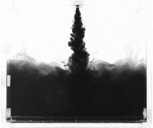
Figure 2. A series of images of a dyed plume from a typical experiment (salt only in this case). The initial descent of the plume is shown in (a); (b,c) show the impact of the fluid on the base and its subsequent rise toward the source, and (d) shows the final steady state with two uniform layers separated by the density interface.
Figure 2 shows a visualisation of a typical single-diffusive experiment, recorded using DigiFlow. The instant when the negatively buoyant axisymmetric turbulent plume, introduced into a fresh stationary ambient from the top, reached the base of the filling box is shown in figure 2(a). During its descent the plume entrained ambient fluid and thus grew in radius. Upon reaching the bottom of the box, the plume spread radially outwards as a gravity current and hit the walls, as shown in figure 2(b). At this moment, the denser fluid began to exit through the bottom opening and was replaced by an equal volume of fresh ambient fluid, entering through the upper openings, to conserve volume. As the volume flux supplied by the plume initially exceeded that imposed by the drainage pump, a layer of salt solution began to form and grew in height, as shown in figure 2(c). This layer continued to increase in depth and density until a steady-state flow was established. Figure 2(d) demonstrates that the steady flow consisted of a two-layer stratification: a fresh upper layer and a well-mixed lower layer of salt solution, separated by a horizontal interface.
As shown in figure 2, the interface between the two layers was not perfectly flat and horizontal throughout the experiment. The disturbances introduced by the plume caused interfacial waves between the fresh and saline layers. As the interface moved closer to the plume source, the amplitude of these interfacial waves reduced, but remained significant compared with the thickness of the interface. As the fluctuations were oscillatory in time, it was necessary to perform multiple measurements of the interface position to average out any temporal variations.
5.1 Conductivity and temperature measurements

Figure 3. Dimensionless conductivity and temperature profiles for experiment HS9. The chronological order of obtained measurements is indicated by the darkness of the lines, with the darker ones corresponding to later profiles. Here the subscripts max and min denote the maximum and minimum values of the variables for this experiment.
Figure 3 shows the outputs of the conductivity probe and thermocouple traversed through the box during the filling process of experiment HS9. Such profiles were typical for all experiments. The chronological order of the measurements is indicated by the darkness of the lines, with the darker lines corresponding to later profiles. The salinity profiles, shown in figure 3(a) can be roughly broken down into three sections from the top down: (i) a region of constant low salinity (top layer); (ii) an intermediate region where the salinity increases to that of the bottom layer; and (iii) a high-salinity region (bottom layer). The sequence of profiles shows that the bottom layer grew in height and salinity during the filling process, until the steady state was reached with the salinity interface fluctuating around its mean position. The associated temperature profiles, shown in figure 3(b), exhibit a similar behaviour, typical for all conducted thermohaline experiments, wherein the temperature of the bottom layer grew until reaching the steady state.
Two important observations about the profiles have to be made here. First, in comparison with the salinity profiles, the outputs of temperature measurements are considerably more diffuse, which cannot be explained by the slow response time of the thermocouple, as further reduction of the traversing speed did not make any noticeable difference to the obtained shape. Such diffuse temperature profiles make the definition of the temperature interface position ambiguous and, therefore, unsuitable for locating the interface. For that reason, salinity profiles only were used to locate the interface. Second, figure 3(a,b) demonstrates a small but persistent gradual increase in the salinity and temperature of the upper layer, respectively. While the salinity profiles appear to be nearly uniform at all times, the temperature in the upper layer forms a stable stratification.
This increase in both scalar properties could be a result of either double diffusion acting across the plume, indicative of the counterbuoyancy flux observed by McDougall (Reference McDougall1983) and Turner (Reference Turner2003), and/or double-diffusive convection occurring along the interface between the layers. It is hard to tell with certainty what is the dominating cause of the thermal stratification, but, given that the temperature difference between the top and bottom layers never exceeded  $3.5\,^{\circ }\text{C}$, its effect on plume buoyancy was negligible. Moreover, the reduction in temperature difference between the ambient and the plume owing to the stratification is small, as at the source the ambient temperature increase had a mean value of
  $1.0\,\%\pm 0.5\,\%$ of
  $\unicode[STIX]{x0394}T_{0}$, where the error is one standard deviation. Further, although the temperature of the plume decreases as it descends, so does the ambient temperature anomaly, and the temperature difference between the plume just above the interface and the initial ambient temperature has a mean value of
  $3.2\,\%\pm 2.6\,\%$.

Figure 4. Evolution of the salinity interface in time  $t$ normalised with the drainage timescale
  $T_{d}$: (a) for four individual experiments normalised by box height
  $H$; (b) for all 13 experiments, conducted at the lowest ventilation volume flux for each experiment, normalised by their respective maximum interface heights
  $z_{max}$.
To locate the instantaneous interface position, a hyperbolic tangent was fitted to each salinity profile and the height at the centre of the fitted profile was used to track the interface migration. Figure 4(a) shows the temporal evolution of the interface height determined in this manner for four different experiments. In this figure, the physical time  $t$ has been normalised with a timescale for emptying the tank
  $T_{d}$ at a constant rate due to the ventilation volume flux
  $Q_{v}$, giving the non-dimensional time scale
 $$\begin{eqnarray}\hat{t}=\frac{t}{T_{d}}=t\;\frac{Q_{v}}{SH},\end{eqnarray}$$
 where  $S$ and
  $H$ are the floor area and height of the tank, respectively. It is clear that for the four (typical) experiments shown, the interface height becomes approximately steady after
  $\hat{t}\simeq 2$.
Figure 4(b) shows the evolution of interface position normalised by the maximum interface distance  $z_{max}$ for all experiments conducted at the lowest ventilation volume flux
  $Q_{v}^{min}=21.8~\text{ml}~\text{s}^{-1}$. In line with figure 4(a), we see that after
  $\hat{t}\simeq 2$ all experiments reached a steady state. We also observed that for ventilation flow rates higher than
  $Q_{v}>Q_{v}^{min}$ the interface reached a steady state faster (in
  $\hat{t}\leqslant 2$), and therefore, for consistency, we took the last six profiles (
 $\hat{t}>2$) for each experiment to calculate the time-averaged steady-state salinity
  $\overline{S}(z)$ and temperature
  $\overline{T}(z)$ profiles using
 $$\begin{eqnarray}\overline{S}(z)=\frac{1}{(i_{e}-i_{s}+1)}\mathop{\sum }_{i_{s}=6}^{i_{e}=11}S_{i}(z)\quad \text{and}\quad \overline{T}(z)=\frac{1}{(i_{e}-i_{s}+1)}\mathop{\sum }_{i_{s}=6}^{i_{e}=11}T_{i}(z).\end{eqnarray}$$
 Figure 5 shows the typical calculated steady-state time-averaged salinity  $\overline{S}(z)$ and temperature
  $\overline{T}(z)$ profiles. The figure demonstrates that the steady-state salinity profile is very well-approximated by the hyperbolic tangent fit and can therefore be used to determine the interface position. The horizontal dashed bars represent the confidence levels of the interface position, estimated by extrapolating the slope at the centre of the interface to the edges of the profile. Although, as noted earlier, the averaged temperature profile is too diffuse to be used for accurate interface identification, figure 5 demonstrates that the temperature increase starts within the confidence levels.

Figure 5. Typical normalised time-averaged steady-state profiles of salinity  $\overline{S}(z/H)$, fitted using hyperbolic tangent profile, and temperature
  $\overline{T}(z/H)$.
5.2 Entrainment coefficient
Figure 6 shows the calculated values of the top-hat entrainment coefficient  $\unicode[STIX]{x1D6FC}$ for three single-diffusive experiments (figure 6a) and four double-diffusive experiments (figure 6b) at five ventilation volume fluxes, evaluated using (3.1). The vertical error bars represent the combination of errors from temporal interface fluctuations, and the uncertainties in the temperature and supply volume flux measurements. These three sources of error were estimated as two standard deviations about their respective mean values for each experiment. Figure 6(a) demonstrates that the value of the entrainment coefficient for single-diffusive plumes is a constant, independent of plume buoyancy flux and ventilation volume flux, with a mean of
  $\unicode[STIX]{x1D6FC}=0.129\pm 0.002$, where the error represents two standard deviations from the mean. This is in good agreement with the generally accepted value of
  $\unicode[STIX]{x1D6FC}\approx 0.13$, reported in various experimental investigations (Linden Reference Linden, Batchelor, Moffatt and Worster2000), and was therefore used as a benchmark for further results.

Figure 6. (a) Top-hat entrainment coefficient  $\unicode[STIX]{x1D6FC}$ for: (a) three single-diffusive experiments at five ventilation volume fluxes
  $Q_{v}$; (b) four double-diffusive experiments at five ventilation volume fluxes
  $Q_{v}$.
In contrast to the results obtained from experiments with single-diffusive plumes, figure 6(b) shows that the values of the entrainment coefficient for double-diffusive plumes are (i) not constant and (ii) smaller than the single-diffusive entrainment constant. These two observations are surprising for a number of reasons. Observation (i) is contradictory to the general assumption that molecular diffusion plays no role in the dynamics of entrainment in high-Péclet-number turbulent plumes. Observation (ii) is also surprising, because we naively supposed that the small-scale double-diffusive processes would enhance mixing of the engulfed fluid, leading to an increase of the effective entrainment coefficient. The observed reduction in the entrainment coefficient cannot be explained by the temporal change in the buoyancy flux of the plume during its descent. The faster diffusion of heat would result in an increase of the negative buoyancy flux, driving the flow, which, in turn, would lead to an increase in the plume volume flux and ‘move’ the interface closer to the source than it should be for a given initial source buoyancy flux  $B_{0}$. From (3.1), this reduction of
  $h$ would yield an increased value of the entrainment coefficient, opposite to our observations.
Two additional important observations have to be made here. First, recalling that the experimental parameters presented in table 1 were tabulated in the ascending order of  $R_{\unicode[STIX]{x1D70C}}$, it is clear that the reduction of the entrainment coefficient is proportional to the strength of the double diffusivity of the plume, represented by
  $R_{\unicode[STIX]{x1D70C}}$. In particular, figure 6(b) shows that for all values of ventilation volume flux
  $Q_{v}$, the values of the entrainment coefficient for HS13 are lower than those of HS11, HS7 and HS5. This suggests that the intensity of the double-diffusive processes within the plume controls the magnitude of the reduction in entrainment. We also observe some non-monotonic behaviour of HS5 and HS7, in that their values of the entrainment coefficient appear to reduce at the intermediate range of
  $Q_{v}$. However, the magnitude of these variations in relation to experimental uncertainty for those experiments, makes it is difficult to comment reliably on this observation.
Second, for highly doubly diffusive experiments (HS11 and HS13), the values of the entrainment coefficient exhibit a clear dependency on the ventilation flux, that is, for smaller values of the flux, the reduction of the entrainment coefficient is greater. Note that, in effect, a reduction in  $Q_{v}$ results in the migration of the interface towards the plume source. Therefore, the second observation can be transformed into a statement that, the reduction in the entrainment coefficient is greater when the interface is closer to the plume source. This observation is not explained by the need for the plume to adjust to a self-similar state, as the lowest ratio of the distance to the interface and jet length is
  $h/L_{m}=6.6$. Instead, this observation suggests that the strength of double diffusion in the plume varies with distance from the source.

Figure 7. Entrainment coefficient results for all experiments at all ventilation volume fluxes as a function of: (a) density ratio  $R_{\unicode[STIX]{x1D70C}}$, where marker colour represents the normalised distance from the plume virtual origin to the interface
  $h/H$; (b) normalised distance from the plume virtual origin to the interface
  $h/H$, where marker colour represents stability ratio
  $R_{\unicode[STIX]{x1D70C}}$.
To explore further the variation of double-diffusive effects within the plume, we present the results in a different fashion in figure 7. Figure 7(a) shows the dependence of the top-hat entrainment coefficient on the density ratio  $R_{\unicode[STIX]{x1D70C}}$ for all experiments at all ventilation fluxes (making a total of 65 data points). The colour scheme in this figure represents the normalised distance from the plume virtual origin to the steady-state interface
  $h/H$. Although no clear dependency between the entrainment coefficient and
  $h$ is observed in the range
  $0<R_{\unicode[STIX]{x1D70C}}<0.3$, there appears to be a pattern for strongly double-diffusive experiments in the range
  $0.3<R_{\unicode[STIX]{x1D70C}}<0.6$. In particular, for a specific value of
  $R_{\unicode[STIX]{x1D70C}}$, the values of entrainment coefficient are consistently smaller for smaller
  $h$, that is, monotonically reducing with
  $h$. The absence of such behaviour in the region
  $0<R_{\unicode[STIX]{x1D70C}}<0.3$ is attributed to the fact that the magnitude of dependence on
  $h$ is comparable with the experimental uncertainty. Figure 7(b) displays the same results as a function of the distance to the interface. As expected, the figure shows that for single-diffusive plumes, represented by the dark blue markers, there is no dependency on the interface position, confirming that the entrainment coefficient is a constant. In contrast, the strongly double-diffusive plumes exhibit a clear dependency on the distance travelled to the interface. The data, displayed in figure 7 lead to the conclusion that double-diffusive effects, acting to inhibit entrainment, vary along the plume and are stronger closer to the plume source. An attempt to explain these observations is made in the following section.
5.3 Differential diffusion mechanism

Figure 8. A schematic snapshot of the edge of a thermohaline negatively buoyant plume during its descent, showing the distribution of vertical velocity  $w(r,z)$, temperature outside salinity edge
  $T_{a}$ and vorticity fields
  $\unicode[STIX]{x1D701}_{p}$ and
  $\unicode[STIX]{x1D701}_{a}$, within and outside the plume, respectively.
One possible explanation for the observed reduction of entrainment is based on differential diffusion of the properties driving the plume motion. Consider a snapshot of a negatively buoyant turbulent thermohaline plume during its descent, schematically illustrated in figure 8. We assume for simplicity that the flux of salt across the salinity interface is negligible, with only heat being transferred from the plume to the surrounding fluid by molecular diffusion (evidence of this heat diffusion across the plume/ambient interface is shown in figure 3b). Under these assumptions, the ambient fluid just outside the salinity interface is fresh and warm, with an associated Gaussian distribution of temperature  $T_{a}$ in the radial direction. Such a temperature profile will create a corresponding buoyancy force distribution, which, in turn, will produce a vorticity field
  $\unicode[STIX]{x1D701}_{a}$, oriented oppositely to the vorticity field
  $\unicode[STIX]{x1D701}_{p}$ within the plume itself. This oppositely orientated vorticity field outside the plume edge
  $\unicode[STIX]{x1D701}_{a}$ will counteract
  $\unicode[STIX]{x1D701}_{p}$ and thereby inhibit turbulent engulfment, which, as discussed in § 1, could be the dominant mechanism of entrainment. This explanation, based on differential diffusion of heat and salt, is consistent with the observations of ‘counterbuoyancy’ fluxes and ‘plume splitting’ made by McDougall (Reference McDougall1983), Turner & Veronis (Reference Turner and Veronis2000) and Turner (Reference Turner2003).
From the above model it follows that the strength of the thermally induced external vorticity field  $\unicode[STIX]{x1D701}_{a}$ is dependent on the temperature gradient at the salinity interface, with larger gradients inducing a stronger field. From our definition of
  $R_{\unicode[STIX]{x1D70C}}$, for a fixed salinity difference, larger values of density ratio
  $R_{\unicode[STIX]{x1D70C}}$ are accompanied by stronger temperature gradients and, thus, the proposed counteracting effect of the external vorticity field on engulfment is greater. This explains the direct relationship between
  $R_{\unicode[STIX]{x1D70C}}$ and the scale of entrainment reduction. Such reasoning is consistent with large-scale engulfment being dominant in the entrainment process.
The proposed explanation also supports the observed inverse dependence of the reduction in entrainment with the distance travelled by the plume. Close to its source, the plume experiences a significant reduction in entrainment, as it has not yet lost its heat and the temperature gradients are still large. As the plume continues its downward motion, exchanging its properties with the ambient, heat is lost  $O(100)$ times faster than salt by the action of molecular diffusion, thereby decreasing the local value of the density ratio from that at the source. This reduction continues as the plume descends.
An estimate of the velocity scale in the region driven by the temperature alone can be constructed as
 $$\begin{eqnarray}w\sim \sqrt{g\unicode[STIX]{x1D6FD}_{T}\unicode[STIX]{x0394}Tb}.\end{eqnarray}$$
 To get an order of magnitude estimate, we take  $g=10~\text{m}~\text{s}^{-2}$,
  $\unicode[STIX]{x1D6FD}_{T}=1{0^{-4}\,}^{\circ }\text{C}^{-1}$ and
  $\unicode[STIX]{x0394}T=1\,^{\circ }\text{C}$. Assuming diffusive growth of the thermal boundary layer (
 $b\sim \sqrt{\unicode[STIX]{x1D705}_{T}t}$), we take
  $b=10^{-3}~\text{m}$. Using these values, the vertical velocity will be
  $O(10^{-3})~\text{m}~\text{s}^{-1}$, which is approximately 10 % of the typical entrainment velocity and, therefore, could hinder the entrainment process.
6 Conclusions
An experimental investigation of the role of double diffusion on the rate of entrainment in turbulent plumes has been conducted. We have restricted our attention to negatively buoyant saline and thermohaline plumes discharged vertically downwards into a stationary uniform freshwater ambient. Under this configuration, the thermohaline plumes were in the salt-fingering regime. As expected, the obtained values of the top-hat entrainment coefficient for single-diffusive (saline) plumes are a constant  $\unicode[STIX]{x1D6FC}=0.129\pm 0.002$, independent of the source buoyancy flux and the ventilation flux
  $Q_{v}$.
However, we observed a reduction in the value of the entrainment coefficient by up to 20 % for double-diffusive thermohaline plumes. The reduction is not explained by the changes in the plume buoyancy flux, as this would yield the opposite result. As shown in figure 7(a), the scale of reduction is in direct relation to the source density ratio  $R_{\unicode[STIX]{x1D70C}}$, indicating that double-diffusive processes alter the dynamics of turbulent entrainment. The reduction is also inversely related to the distance from the virtual origin to the interface
  $h$, implying transiency of the double-diffusive effects. The exact functional relationship of
  $\unicode[STIX]{x1D6FC}$ as a function of
  $z$ and
  $R_{\unicode[STIX]{x1D70C}}$ remains to be established. As all of our experiments were in the salt-fingering configuration, it is also unclear at this stage as to what effect double-diffusion would have on the dynamics of a plume in the diffusive regime.
There are at least two important implications of this paper. First, our findings may be useful in deciding whether double-diffusive effects would be of importance in modelling entrainment and subsequent dynamics of turbulent plumes in various environmental and industrial scenarios. Extrapolation to large-scale systems requires independence of the flow on Péclet and Reynolds numbers. Previously noted agreement between heat-only and salt-only plumes shows that these plumes are already independent of  $Pe$ and it is well known that laboratory-scale plumes at lower
  $Re$ capture the dynamics of large-scale plumes (Briggs Reference Briggs1982). One particular example is the already mentioned case of an iceberg melting, the typical temperature and salinity differences between the produced meltwater and the ambient ocean are
  $\unicode[STIX]{x0394}T=5\,^{\circ }\text{C}$ and
  $\unicode[STIX]{x0394}S=0.035$, respectively, yielding a density ratio of
  $R_{\unicode[STIX]{x1D70C}}=0.05$. Based on our experimental results, such a low source density ratio would result in a minor reduction in the entrainment coefficient. However, for cases where
  $R_{\unicode[STIX]{x1D70C}}$ is significantly greater, the double-diffusive effects should not be ignored. Second, this article has shown that even for high-Péclet-number turbulent flows, in which advection dominates diffusion, the effect of molecular diffusion can be non-negligible, as it may alter the overall dynamics of the flow.
Acknowledgements
We acknowledge funding from the EPSRC under the Programme Grant EP/K034529/1 ‘Mathematical Underpinnings of Stratified Turbulence’ (MUST), and from the European Research Council (ERC) under the European Union’s Horizon 2020 research and innovation programme under grant no. 742480 ‘Stratified Turbulence And Mixing Processes’ (STAMP). M.D. is supported by the Gates Cambridge Scholarship. We are grateful for the invaluable experimental support of Professor S. Dalziel and of the technicians of the G. K. Batchelor Laboratory.
Declaration of interests
The authors report no conflict of interest.
Appendix A
To verify that the conductive heat losses were insignificant, a series of experiments measuring the thermal conductivity of the filling box were performed. To this end, we determined the effective heat transfer coefficient  $U$ of the container, which enters the rate of conductive heat loss relation as
 $$\begin{eqnarray}H_{c}=U\unicode[STIX]{x0394}TA_{T},\end{eqnarray}$$
 where  $A_{T}$ is the total conductive surface area, and
  $\unicode[STIX]{x0394}T=T_{H}-T_{C}$ is the temperature difference between the interior and the exterior of the box.
The experiments were performed by filling the box with hot fluid, and then sealing it and placing it inside the environmental tank to cool. An array of four T-type thermocouples with 40 mm vertical spacing was placed inside the box and another two into the ambient fluid to monitor the temperature difference. A magnetic stirrer was inserted into the box to keep the interior well-mixed. A schematic representation of the experimental arrangement is shown in figure 9. From the obtained temperature measurements, we estimated the value of  $U$ using Newton’s law of cooling, in the form
 $$\begin{eqnarray}\unicode[STIX]{x1D703}=\exp (-\unicode[STIX]{x1D6FE}t),\end{eqnarray}$$
 where  $\unicode[STIX]{x1D703}=T-T_{C}/T_{0}-T_{C}$ is the non-dimensional temperature,
  $\unicode[STIX]{x1D6FE}=A_{T}U/mc_{p}$,
  $m$ is the mass of warm fluid and
  $c_{p}$ is the specific heat capacity of water.

Figure 9. A schematic representation of the conductive heat-loss experiment.

Figure 10. Time evolution of: (a) temperature differences  $T_{H}-T_{C}$ between the interior and exterior of the box; (b) normalised temperature differences
  $\unicode[STIX]{x1D703}$ between the interior and exterior of the box. Plot (b) shows good collapse of the obtained measurements from four different experiments.
Two pairs of experiments, with hot water levels of  $h_{T}=0.195~\text{m}$ and
  $h_{T}=0.245~\text{m}$, respectively, were performed. Figure 10 demonstrates the time series of the obtained temperature measurements. On both plots, the lines represent the average readings from thermocouples inside and outside the tank, with respective accuracies of
  $\pm 0.16\,^{\circ }\text{C}$ and
  $\pm 0.12\,^{\circ }\text{C}$, estimated as two standard deviations of the time-average fluctuations between thermocouple readings. Such a small error shows that both the interior of the tank and the fluid in the larger environmental tank remained well-mixed throughout the experiment. Figure 10(a) demonstrates that, as expected, the temperature difference between the interior and the exterior of the tank decays exponentially. Normalising the temperature differences to obtain
  $\unicode[STIX]{x1D703}$ and plotting it on a logarithmic
  $y$-scale, as shown in figure 10(b), we obtain a linear decay in time, whose gradient represents the value of
  $\unicode[STIX]{x1D6FE}$. By performing a linear fit for the obtained measurements of
  $\unicode[STIX]{x1D703}$ and substituting the obtained values of the gradient into the relation for
  $\unicode[STIX]{x1D6FE}$ we found a
  $U$-value of
  $18.5\pm 0.3~\text{W}~\text{m}^{-2}~\text{K}$, where the error represents two standard deviations around the mean of the four obtained results.
Using the experimentally obtained  $U$-value for the filling box, we estimated conductive heat losses
  $H_{c}$ using (A 1). In this calculation, we used an appropriate
  $A_{T}$, based on the interface height, and assumed that the bottom layer is well-mixed with its temperature equal to the temperature measured at the bottom of the box
  $T_{b}$. The obtained losses were compared with the thermal flux into the box from the supply nozzle, defined as
 $$\begin{eqnarray}H_{in}={\dot{m}}_{in}c_{p}(T_{in}-T_{amb}),\end{eqnarray}$$
 where  ${\dot{m}}_{in}$ is the mass flux of the supply fluid, and
  $T_{in}$ and
  $T_{amb}$ are the temperatures of the supply fluid and the ambient, respectively. In this way, we estimated that the typical thermal losses by conduction through the side tank walls
  $H_{loss}$ were up to
  $3.0\pm 0.3\,\%$ of the total heat input
  $H_{in}$, confirming that the heat losses were insignificant and did not have an impact on the experimental results.
As a further check of the experimental data, we performed the heat budget of each experiment, which, assuming no losses, can be written as
 $$\begin{eqnarray}Q_{0}T_{in}+(Q_{v}-Q_{0})T_{amb}=Q_{v}T_{b}.\end{eqnarray}$$
 We find that the overall heat budget for all filling-box experiments is accurate up to  $14.5\,\%\pm 0.4\,\%$. However, this is extremely sensitive to temperature differences, that is, a change by
  $0.3\,^{\circ }\text{C}$ only, comparable with the uncertainty of the temperature measurements, would result in a perfect balance.


