


1. Introduction
The case of turbulent wall-bounded flow over rough surfaces has been extensively studied, owing to important practical implications. Such flows almost always produce skin-friction coefficients,
 $C_{f}$
(which is the ratio between the wall shear stress
$C_{f}$
(which is the ratio between the wall shear stress
 ${\it\tau}_{w}$
and the dynamic pressure
${\it\tau}_{w}$
and the dynamic pressure
 ${\it\rho}U_{b}^{2}/2$
, where
${\it\rho}U_{b}^{2}/2$
, where
 $U_{b}$
is the bulk velocity and
$U_{b}$
is the bulk velocity and
 ${\it\rho}$
the density of the fluid), that are higher than those of smooth surfaces, and are thus of concern in a wide range of applications. For example, biofouling on a ship’s hull roughens the surface, causing an increase in the drag which consequently decreases the fuel efficiency of the ship (see for example Schultz et al.
Reference Schultz, Bendick, Holm and Hertel2011). Roughness is also an important factor in meteorological flows, where the atmospheric surface layer encounters changes in surface topology owing to vegetation canopies, man-made structures and ocean waves (Thom Reference Thom1971; Raupach & Shaw Reference Raupach and Shaw1982; Raupach, Antonia & Rajagopalan Reference Raupach, Antonia and Rajagopalan1991; Yang, Meneveau & Shen Reference Yang, Meneveau and Shen2013). In biomedical flows also, roughness can occur as plaque build-up in arteries, and as a result of the stents that are used to treat such conditions (see for example Cunningham & Gotlieb Reference Cunningham and Gotlieb2004).
${\it\rho}$
the density of the fluid), that are higher than those of smooth surfaces, and are thus of concern in a wide range of applications. For example, biofouling on a ship’s hull roughens the surface, causing an increase in the drag which consequently decreases the fuel efficiency of the ship (see for example Schultz et al.
Reference Schultz, Bendick, Holm and Hertel2011). Roughness is also an important factor in meteorological flows, where the atmospheric surface layer encounters changes in surface topology owing to vegetation canopies, man-made structures and ocean waves (Thom Reference Thom1971; Raupach & Shaw Reference Raupach and Shaw1982; Raupach, Antonia & Rajagopalan Reference Raupach, Antonia and Rajagopalan1991; Yang, Meneveau & Shen Reference Yang, Meneveau and Shen2013). In biomedical flows also, roughness can occur as plaque build-up in arteries, and as a result of the stents that are used to treat such conditions (see for example Cunningham & Gotlieb Reference Cunningham and Gotlieb2004).
The increase in wall drag caused by the surface roughness is manifested in the streamwise mean velocity profile as a downward shift in the logarithmic region,
 ${\rm\Delta}U^{+}\equiv {\rm\Delta}U/U_{{\it\tau}}$
(
${\rm\Delta}U^{+}\equiv {\rm\Delta}U/U_{{\it\tau}}$
(
 $U_{{\it\tau}}\equiv \sqrt{{\it\tau}_{w}/{\it\rho}}$
, the friction velocity), known as the roughness function. The roughness function is itself a function of the roughness Reynolds number,
$U_{{\it\tau}}\equiv \sqrt{{\it\tau}_{w}/{\it\rho}}$
, the friction velocity), known as the roughness function. The roughness function is itself a function of the roughness Reynolds number,
 $k^{+}=kU_{{\it\tau}}/{\it\nu}$
, where
$k^{+}=kU_{{\it\tau}}/{\it\nu}$
, where
 $k$
is some measure of the roughness height and
$k$
is some measure of the roughness height and
 ${\it\nu}$
is the kinematic viscosity. Note that for rough-wall flows,
${\it\nu}$
is the kinematic viscosity. Note that for rough-wall flows,
 $U_{{\it\tau}}$
and
$U_{{\it\tau}}$
and
 $C_{f}$
are no longer composed solely of the skin-friction drag but actually reflect the total wall drag which is composed of viscous and pressure drag components. The engineering challenge is to predict the roughness function for a given surface at operational conditions. If this is known, engineers can predict the drag coefficient and hence the energy requirements or penalty due to the surface roughness, either using the Moody chart (Moody Reference Moody1944) for pipes and channels, or variants of this for developing turbulent boundary layers (Prandtl & Schlichting Reference Prandtl and Schlichting1955; Granville Reference Granville1958). It should be noted that both of these approaches require an assumed self-similar functional form for the mean velocity profile. Hence the existence of outer-layer similarity (Townsend Reference Townsend1980) for rough flows is pivotal to the process of extrapolating laboratory results to full-scale applications.
$C_{f}$
are no longer composed solely of the skin-friction drag but actually reflect the total wall drag which is composed of viscous and pressure drag components. The engineering challenge is to predict the roughness function for a given surface at operational conditions. If this is known, engineers can predict the drag coefficient and hence the energy requirements or penalty due to the surface roughness, either using the Moody chart (Moody Reference Moody1944) for pipes and channels, or variants of this for developing turbulent boundary layers (Prandtl & Schlichting Reference Prandtl and Schlichting1955; Granville Reference Granville1958). It should be noted that both of these approaches require an assumed self-similar functional form for the mean velocity profile. Hence the existence of outer-layer similarity (Townsend Reference Townsend1980) for rough flows is pivotal to the process of extrapolating laboratory results to full-scale applications.
Typically, the roughness function is predicted empirically, by testing a replica of the surface roughness in the laboratory. Measurements of the mean velocity profile within the turbulent boundary layer enable the determination of
 ${\rm\Delta}U^{+}$
as a function of the roughness Reynolds number. Alternatively, drag measurements on towed test surfaces, or pressure drop measurements in roughened pipes or channels also enable a determination of the coefficient of friction
${\rm\Delta}U^{+}$
as a function of the roughness Reynolds number. Alternatively, drag measurements on towed test surfaces, or pressure drop measurements in roughened pipes or channels also enable a determination of the coefficient of friction
 $C_{f}$
and hence, via assumptions of self-similar velocity profiles,
$C_{f}$
and hence, via assumptions of self-similar velocity profiles,
 ${\rm\Delta}U^{+}$
. The key point is that the relationship between
${\rm\Delta}U^{+}$
. The key point is that the relationship between
 ${\rm\Delta}U^{+}$
and
${\rm\Delta}U^{+}$
and
 $k^{+}$
is highly dependent on the characteristics of the surface and is not trivial, requiring engineers to conduct scaled experiments in order to predict full-scale performance. An overarching goal for roughness research would be to bypass this costly empirical stage, and to produce a methodology that is capable of predicting the relationship between
$k^{+}$
is highly dependent on the characteristics of the surface and is not trivial, requiring engineers to conduct scaled experiments in order to predict full-scale performance. An overarching goal for roughness research would be to bypass this costly empirical stage, and to produce a methodology that is capable of predicting the relationship between
 ${\rm\Delta}U^{+}$
and
${\rm\Delta}U^{+}$
and
 $k^{+}$
directly from known characteristics of the surface. In the past, many such attempts have been made, occasionally suggesting new roughness parameters in order to characterise the surface. Jimenez (Reference Jimenez2004) and Flack & Schultz (Reference Flack and Schultz2010) provide overviews of some of these schemes. Schlichting (Reference Schlichting1936) introduces the solidity parameter,
$k^{+}$
directly from known characteristics of the surface. In the past, many such attempts have been made, occasionally suggesting new roughness parameters in order to characterise the surface. Jimenez (Reference Jimenez2004) and Flack & Schultz (Reference Flack and Schultz2010) provide overviews of some of these schemes. Schlichting (Reference Schlichting1936) introduces the solidity parameter,
 ${\it\Lambda}$
, defined as the total projected frontal roughness area per unit wall-parallel area. It has been a key parameter for characterising the effect of various regular rough surfaces, such as spheres, cones, spherical segments and spanwise fences.
${\it\Lambda}$
, defined as the total projected frontal roughness area per unit wall-parallel area. It has been a key parameter for characterising the effect of various regular rough surfaces, such as spheres, cones, spherical segments and spanwise fences.
More recently, Napoli, Armenio & De Marchis (Reference Napoli, Armenio and De Marchis2008) who conducted numerical simulations on channels with two-dimensional inhomogeneous roughness, suggest that the effective slope
 $\mathit{ES}$
, defined as the mean absolute streamwise gradient of the surface, scales well with
$\mathit{ES}$
, defined as the mean absolute streamwise gradient of the surface, scales well with
 ${\rm\Delta}U^{+}$
for a variety of non-regular rough walls, independent of the roughness height. On the contrary, in a boundary layer experiment Schultz & Flack (Reference Schultz and Flack2009) found that
${\rm\Delta}U^{+}$
for a variety of non-regular rough walls, independent of the roughness height. On the contrary, in a boundary layer experiment Schultz & Flack (Reference Schultz and Flack2009) found that
 ${\rm\Delta}U^{+}$
is sensitive to the roughness height and independent of
${\rm\Delta}U^{+}$
is sensitive to the roughness height and independent of
 $\mathit{ES}$
if the surface has large values of
$\mathit{ES}$
if the surface has large values of
 $\mathit{ES}\;({>}0.35)$
. Other work has suggested that combinations of more traditional surface roughness parameters can yield predictions of
$\mathit{ES}\;({>}0.35)$
. Other work has suggested that combinations of more traditional surface roughness parameters can yield predictions of
 ${\rm\Delta}U^{+}$
. For example, Flack & Schultz (Reference Flack and Schultz2010) propose that the equivalent sand grain roughness can be modelled as a function of the root-mean-square roughness height
${\rm\Delta}U^{+}$
. For example, Flack & Schultz (Reference Flack and Schultz2010) propose that the equivalent sand grain roughness can be modelled as a function of the root-mean-square roughness height
 $k_{rms}$
and skewness
$k_{rms}$
and skewness
 $k_{sk}$
. This proposed model works very well in predicting the equivalent sand grain roughness
$k_{sk}$
. This proposed model works very well in predicting the equivalent sand grain roughness
 $k_{s}$
of gravel, packed spheres covered with grit and sandpaper (12 and 80 grit) in the fully rough regime. On the other hand, the model overpredicts
$k_{s}$
of gravel, packed spheres covered with grit and sandpaper (12 and 80 grit) in the fully rough regime. On the other hand, the model overpredicts
 $k_{s}$
for honed and commercial pipes by approximately 100 %. Though some of these models have proven promising for certain classes of surfaces, none has proven universally reliable (refer to Flack & Schultz Reference Flack and Schultz2010 for further information on previously proposed roughness function correlations). Taylor, Coleman & Hodge (Reference Taylor, Coleman and Hodge1985) characterised the rough surface using a discrete element model for uniform roughness. In this model, the coefficient of friction of the surface can be estimated by modelling the coefficient of drag
$k_{s}$
for honed and commercial pipes by approximately 100 %. Though some of these models have proven promising for certain classes of surfaces, none has proven universally reliable (refer to Flack & Schultz Reference Flack and Schultz2010 for further information on previously proposed roughness function correlations). Taylor, Coleman & Hodge (Reference Taylor, Coleman and Hodge1985) characterised the rough surface using a discrete element model for uniform roughness. In this model, the coefficient of friction of the surface can be estimated by modelling the coefficient of drag
 $C_{D}$
of the individual roughness elements. This model has been used on sphere- and cone-roughened surfaces and is able to accurately predict the skin-friction coefficient of a surface
$C_{D}$
of the individual roughness elements. This model has been used on sphere- and cone-roughened surfaces and is able to accurately predict the skin-friction coefficient of a surface
 $C_{f}$
(Scaggs, Taylor & Coleman Reference Scaggs, Taylor and Coleman1988). However, for more complex, realistic-looking rough surfaces,
$C_{f}$
(Scaggs, Taylor & Coleman Reference Scaggs, Taylor and Coleman1988). However, for more complex, realistic-looking rough surfaces,
 $C_{D}$
is not easily determined unless an experiment is carried out.
$C_{D}$
is not easily determined unless an experiment is carried out.
To achieve the aim of predicting the drag of a surface without conducting laboratory experiments, a better understanding of roughness is needed. It is important to know how the flow is affected by certain key roughness parameters. In the present study, we take a simple building-block roughness (which could later form the basis of a decomposition of a more complex geometry), and investigate the influence of the wavelength of the inner-normalised roughness elements
 ${\it\lambda}^{+}$
, and also the roughness semi-amplitude height
${\it\lambda}^{+}$
, and also the roughness semi-amplitude height
 $h^{+}$
. By systematically varying these parameters, we are also able to investigate the influence of solidity
$h^{+}$
. By systematically varying these parameters, we are also able to investigate the influence of solidity
 ${\it\Lambda}$
and effective slope
${\it\Lambda}$
and effective slope
 $\mathit{ES}$
. The aim here is to take a more systematic approach in the spirit of the close-packed pyramids experiments of Schultz & Flack (Reference Schultz and Flack2009) and the
$\mathit{ES}$
. The aim here is to take a more systematic approach in the spirit of the close-packed pyramids experiments of Schultz & Flack (Reference Schultz and Flack2009) and the
 $\mathit{ES}$
simulations of Napoli et al. (Reference Napoli, Armenio and De Marchis2008) towards producing more reliable predictive schemes.
$\mathit{ES}$
simulations of Napoli et al. (Reference Napoli, Armenio and De Marchis2008) towards producing more reliable predictive schemes.
In this study, direct numerical simulation (DNS) with a body-fitted grid is used to simulate the flow through a pipe roughened with three-dimensional sinusoidal elements at low Reynolds number. A body-fitted grid was chosen in favour of the immersed boundary method (IBM) to remove uncertainties in the near-wall flow which may arise due to the unphysical oscillations occurring in the vicinity of the virtual boundary (Iaccarino & Verzicco Reference Iaccarino and Verzicco2003). However, a turbulent rough-wall simulation with a body-fitted grid is computationally more expensive. The current simulation at
 $\mathit{Re}_{{\it\tau}}=540$
requires 120 268 800 elements as compared to 35 000 000 nodes for an open channel simulation by Leonardi & Castro (Reference Leonardi and Castro2010) at comparable Reynolds number (
$\mathit{Re}_{{\it\tau}}=540$
requires 120 268 800 elements as compared to 35 000 000 nodes for an open channel simulation by Leonardi & Castro (Reference Leonardi and Castro2010) at comparable Reynolds number (
 $\mathit{Re}_{{\it\tau}}=600$
) using IBM. For the current simulations, a decision has been made balancing the need for high Reynolds number and the need to investigate a range of surfaces using body-fitted grids. Based on the strong belief that a large number of simulations covering a wide surface parameter space would produce more insight into the problem than a limited number of simulations at high Reynolds numbers, we elect after careful validation, to perform the majority of simulations at low Reynolds numbers. For comparison, the computational hours required for a rough-wall simulation at
$\mathit{Re}_{{\it\tau}}=600$
) using IBM. For the current simulations, a decision has been made balancing the need for high Reynolds number and the need to investigate a range of surfaces using body-fitted grids. Based on the strong belief that a large number of simulations covering a wide surface parameter space would produce more insight into the problem than a limited number of simulations at high Reynolds numbers, we elect after careful validation, to perform the majority of simulations at low Reynolds numbers. For comparison, the computational hours required for a rough-wall simulation at
 $\mathit{Re}_{{\it\tau}}=180$
would only be approximately 43 000 CPU hours using 256 Blue Gene/Q processors while a simulation at
$\mathit{Re}_{{\it\tau}}=180$
would only be approximately 43 000 CPU hours using 256 Blue Gene/Q processors while a simulation at
 $\mathit{Re}_{{\it\tau}}=540$
would require 1370 000 CPU hours using 1024 Blue Gene/Q processors if the statistics were collected for the same amount of time. This computational burden can easily double for surfaces with large roughness, where a smaller timestep
$\mathit{Re}_{{\it\tau}}=540$
would require 1370 000 CPU hours using 1024 Blue Gene/Q processors if the statistics were collected for the same amount of time. This computational burden can easily double for surfaces with large roughness, where a smaller timestep
 ${\rm\Delta}t$
has to be used (to ensure that the Courant number is approximately 0.8) and the lower bulk velocity
${\rm\Delta}t$
has to be used (to ensure that the Courant number is approximately 0.8) and the lower bulk velocity
 $U_{b}$
means that the flow has to be simulated for a longer duration to obtain converged statistics. In § 4.3, we carefully investigate the validity of the choice of low Reynolds number simulations and we observe only minor differences in the calculated roughness function
$U_{b}$
means that the flow has to be simulated for a longer duration to obtain converged statistics. In § 4.3, we carefully investigate the validity of the choice of low Reynolds number simulations and we observe only minor differences in the calculated roughness function
 ${\rm\Delta}U^{+}$
and similarity in the outer region. In addition, we validate that the
${\rm\Delta}U^{+}$
and similarity in the outer region. In addition, we validate that the
 $\mathit{Re}_{{\it\tau}}=180$
simulation successfully captures the variation in
$\mathit{Re}_{{\it\tau}}=180$
simulation successfully captures the variation in
 ${\rm\Delta}U^{+}$
caused by parametric changes to the surface. Based on these results, a strategic decision is made to simulate the majority of the flows at
${\rm\Delta}U^{+}$
caused by parametric changes to the surface. Based on these results, a strategic decision is made to simulate the majority of the flows at
 $\mathit{Re}_{{\it\tau}}=180$
to ensure that a comprehensive range of test cases can be conducted. It should be highlighted that the roughness cases simulated here are predominantly within the transitionally rough regime. This regime is interesting since it covers the transition from the smooth-wall regime, where viscous drag dominates as a result of the well-known near-wall cycle, to the fully rough regime, where the drag coefficient becomes Reynolds number independent and the pressure drag from the roughness elements is presumed to dominate.
$\mathit{Re}_{{\it\tau}}=180$
to ensure that a comprehensive range of test cases can be conducted. It should be highlighted that the roughness cases simulated here are predominantly within the transitionally rough regime. This regime is interesting since it covers the transition from the smooth-wall regime, where viscous drag dominates as a result of the well-known near-wall cycle, to the fully rough regime, where the drag coefficient becomes Reynolds number independent and the pressure drag from the roughness elements is presumed to dominate.
While there has been extensive numerical study of turbulent flows in smooth-wall pipes (Eggels et al. Reference Eggels, Unger, Weiss, Westerweel, Adrian, Friedrich and Nieuwstadt1994; Loulou et al. Reference Loulou, Moser, Mansour and Cantwell1997; Satake, Kunugi & Himeno Reference Satake, Kunugi and Himeno2000; Wagner, Hüttl & Friedrich Reference Wagner, Hüttl and Friedrich2001; Wu & Moin Reference Wu and Moin2008; Chin et al. Reference Chin, Ooi, Marusic and Blackburn2010; Saha et al. Reference Saha, Chin, Blackburn and Ooi2011), there is limited literature for a turbulent flow in a rough-wall pipe. Simulation of a turbulent flow in a pipe with two-dimensional roughness was conducted by Blackburn, Ooi & Chong (Reference Blackburn, Ooi and Chong2007) where the effects of the corrugation height for a fixed corrugation wavelength were investigated. They found that flow separation occurs when the corrugation height increases and that the pressure drag accounts for approximately 85 % of the total pressure drop in the turbulent flow. To the best of the authors’ knowledge, the present work is the first simulation using a body-conforming grid of turbulent flow within a pipe with three-dimensional roughness elements.
The choice of sinusoidal roughness elements was influenced by the recent work of Mejia-Alvarez & Christensen (Reference Mejia-Alvarez and Christensen2010). In that study, the authors conducted experiments on a realistic rough surface that was scanned and replicated from a turbine blade that had experienced pitting during operation. They decomposed this surface into a series of basis functions, following which they tested the ability of a reconstructed surface, generated from a limited subset of the most energetic modes, to recreate key flow parameters. Building from this background, one future direction we plan to pursue with the current sinusoidal roughness would be to superimpose several modes of different height, wavelength and phase to build towards modelling more complex and hence realistic rough surfaces. However, the first step with such an approach is to understand the single mode, which is rigorously detailed here.
Throughout this paper, we adopt the cylindrical coordinate system where
 $r$
is the radial direction measured from the centre of the pipe,
$r$
is the radial direction measured from the centre of the pipe,
 ${\it\theta}$
is the azimuthal angle and
${\it\theta}$
is the azimuthal angle and
 $x$
is in the streamwise direction. As pointed out by Monty et al. (Reference Monty, Hutchins, Ng, Marusic and Chong2009), the ‘spanwise’ (azimuthal) length scale of the coherent structures in the pipe is measured along the arclength
$x$
is in the streamwise direction. As pointed out by Monty et al. (Reference Monty, Hutchins, Ng, Marusic and Chong2009), the ‘spanwise’ (azimuthal) length scale of the coherent structures in the pipe is measured along the arclength
 $s=r{\it\theta}$
. Capitalised variables (e.g.
$s=r{\it\theta}$
. Capitalised variables (e.g.
 $U$
) indicate time- and plane-averaged quantities, referred to as the global average. Over-bars indicate time-averaged quantities (e.g.
$U$
) indicate time- and plane-averaged quantities, referred to as the global average. Over-bars indicate time-averaged quantities (e.g.
 $\overline{u}$
), and angle brackets indicate in-fluid averages at fixed wall-normal locations (e.g.
$\overline{u}$
), and angle brackets indicate in-fluid averages at fixed wall-normal locations (e.g.
 $\langle u\rangle$
). Lower-case primed symbols (e.g.
$\langle u\rangle$
). Lower-case primed symbols (e.g.
 $u^{\prime }$
) denote fluctuations about the global average and the subscript ‘rms’ denotes the corresponding root-mean-square fluctuations. The ‘
$u^{\prime }$
) denote fluctuations about the global average and the subscript ‘rms’ denotes the corresponding root-mean-square fluctuations. The ‘
 $+$
’ superscript is used to denote viscous scalings of length (e.g.
$+$
’ superscript is used to denote viscous scalings of length (e.g.
 $r^{+}=rU_{{\it\tau}}/{\it\nu}$
), velocity (e.g.
$r^{+}=rU_{{\it\tau}}/{\it\nu}$
), velocity (e.g.
 $u^{+}=u/U_{{\it\tau}}$
) and time (e.g.
$u^{+}=u/U_{{\it\tau}}$
) and time (e.g.
 $t^{+}=tU_{{\it\tau}}^{2}/{\it\nu}$
).
$t^{+}=tU_{{\it\tau}}^{2}/{\it\nu}$
).

Figure 1. (a) Sketch of the rough-wall pipe for case 20\_141. The radial distance
 $r$
is measured from the centre of the pipe whereas
$r$
is measured from the centre of the pipe whereas
 $y$
is measured from the virtual origin of the pipe wall:
$y$
is measured from the virtual origin of the pipe wall:
 $y=(R_{0}-r-{\it\epsilon})/R_{0}$
where
$y=(R_{0}-r-{\it\epsilon})/R_{0}$
where
 ${\it\epsilon}$
is the offset of the virtual origin from the reference radius of the pipe. The four planes labelled
${\it\epsilon}$
is the offset of the virtual origin from the reference radius of the pipe. The four planes labelled
 $I$
,
$I$
,
 $II$
,
$II$
,
 $A$
and
$A$
and
 $B$
will be referred to in the subsequent discussion.
$B$
will be referred to in the subsequent discussion.
 $I$
: rough cross-sectional plane;
$I$
: rough cross-sectional plane;
 $II$
: ‘smooth’ cross-sectional plane;
$II$
: ‘smooth’ cross-sectional plane;
 $A$
: rough streamwise plane; and
$A$
: rough streamwise plane; and
 $B$
: ‘smooth’ streamwise plane.
$B$
: ‘smooth’ streamwise plane.
 $L_{x}$
is the length of the computational domain. (b) O-grid mesh along plane
$L_{x}$
is the length of the computational domain. (b) O-grid mesh along plane
 $I$
, down-sampled by approximately 4.5:1 for clarity. (c) Zoomed in view of the cross-sectional plane illustrating the averaging annulus.
$I$
, down-sampled by approximately 4.5:1 for clarity. (c) Zoomed in view of the cross-sectional plane illustrating the averaging annulus.
2. Numerical procedure
The turbulent flow through a pipe is simulated by solving the Navier–Stokes equations for incompressible flow in Cartesian coordinates:
 $$\begin{eqnarray}\displaystyle & \boldsymbol{{\rm\nabla}}\boldsymbol{\cdot }\boldsymbol{u}=0, & \displaystyle\end{eqnarray}$$
 $$\begin{eqnarray}\displaystyle & \displaystyle \frac{\partial \boldsymbol{u}}{\partial t}+\boldsymbol{u}\boldsymbol{\cdot }\boldsymbol{{\rm\nabla}}\boldsymbol{u}=-\frac{1}{{\it\rho}}\boldsymbol{{\rm\nabla}}p+{\it\nu}{\rm\nabla}^{2}\boldsymbol{u}+F_{x}\boldsymbol{i}, & \displaystyle\end{eqnarray}$$
 $\boldsymbol{u}=(u,v,w)$
is the velocity in the
$\boldsymbol{u}=(u,v,w)$
is the velocity in the
 $x$
,
$x$
,
 $y$
, and
$y$
, and
 $z$
directions,
$z$
directions,
 $t$
is the time and
$t$
is the time and
 $F_{x}(t)$
is the uniform, time-varying body force required to maintain a constant mass flux through the pipe. The flows were simulated using CDP, a finite-volume unstructured-grid code (Ham & Iaccarino Reference Ham and Iaccarino2004; Mahesh, Constantinescu & Moin Reference Mahesh, Constantinescu and Moin2004), where the diffusive and convective terms are advanced in time using the second-order, fully implicit Crank–Nicolson scheme, and continuity is enforced by the fractional-step method by Kim & Moin (Reference Kim and Moin1985).
$F_{x}(t)$
is the uniform, time-varying body force required to maintain a constant mass flux through the pipe. The flows were simulated using CDP, a finite-volume unstructured-grid code (Ham & Iaccarino Reference Ham and Iaccarino2004; Mahesh, Constantinescu & Moin Reference Mahesh, Constantinescu and Moin2004), where the diffusive and convective terms are advanced in time using the second-order, fully implicit Crank–Nicolson scheme, and continuity is enforced by the fractional-step method by Kim & Moin (Reference Kim and Moin1985).
For pipe-flow simulations, the finite-volume grid is typically aligned with cylindrical coordinates. That is, the vertices of the cells coincide with the
 $r$
and
$r$
and
 ${\it\theta}$
coordinates. However, to ensure adequate resolution at the wall, especially in the azimuthal direction, this grid would result in a significant and unnecessary number of cells in the centre of the pipe. Hence, the Navier–Stokes equations are solved in Cartesian coordinates on an ‘O-grid’ mesh. In the centre region of the pipe a square-based grid is employed which transitions to a cylindrical-based grid at the near-wall regions (refer to figure 1). Care has been taken at the transition to ensure that cells are not significantly skewed. The grid is uniformly spaced in the streamwise direction and a linear expansion is used in the radial direction to ensure sufficient resolution at the wall of the pipe. At the centre of the pipe, the cells are approximately cube shaped (
${\it\theta}$
coordinates. However, to ensure adequate resolution at the wall, especially in the azimuthal direction, this grid would result in a significant and unnecessary number of cells in the centre of the pipe. Hence, the Navier–Stokes equations are solved in Cartesian coordinates on an ‘O-grid’ mesh. In the centre region of the pipe a square-based grid is employed which transitions to a cylindrical-based grid at the near-wall regions (refer to figure 1). Care has been taken at the transition to ensure that cells are not significantly skewed. The grid is uniformly spaced in the streamwise direction and a linear expansion is used in the radial direction to ensure sufficient resolution at the wall of the pipe. At the centre of the pipe, the cells are approximately cube shaped (
 ${\rm\Delta}r^{+}\approx {\rm\Delta}r{\it\theta}^{+}\approx {\rm\Delta}x^{+}$
). The size of the grid elements in the rough cases at
${\rm\Delta}r^{+}\approx {\rm\Delta}r{\it\theta}^{+}\approx {\rm\Delta}x^{+}$
). The size of the grid elements in the rough cases at
 $\mathit{Re}_{{\it\tau}}=180$
is approximately 20 % smaller in
$\mathit{Re}_{{\it\tau}}=180$
is approximately 20 % smaller in
 $r$
,
$r$
,
 ${\it\theta}$
and
${\it\theta}$
and
 $x$
than the smooth-wall case to accurately capture the shape of the roughness elements. In addition, the rough surface skews the grid cells near the wall, thus requiring additional grid points to resolve the flow. The skewness of the grid at the wall also limits the roughness-height-to-wavelength ratio,
$x$
than the smooth-wall case to accurately capture the shape of the roughness elements. In addition, the rough surface skews the grid cells near the wall, thus requiring additional grid points to resolve the flow. The skewness of the grid at the wall also limits the roughness-height-to-wavelength ratio,
 $h/{\it\lambda}_{x}$
that can be simulated. Computational details regarding the mean grid spacing near the wall for each case are given in table 1.
$h/{\it\lambda}_{x}$
that can be simulated. Computational details regarding the mean grid spacing near the wall for each case are given in table 1.
Table 1. Computational details for the different roughness cases.
 $N_{r,{\it\theta}}$
is the number of elements in an
$N_{r,{\it\theta}}$
is the number of elements in an
 $(r,{\it\theta})$
plane,
$(r,{\it\theta})$
plane,
 $N_{x}$
is the number of elements in the streamwise direction and
$N_{x}$
is the number of elements in the streamwise direction and
 $N_{{\it\lambda}_{x}}$
is the number of elements per roughness wavelength.
$N_{{\it\lambda}_{x}}$
is the number of elements per roughness wavelength.
 ${\rm\Delta}r^{+}$
,
${\rm\Delta}r^{+}$
,
 ${\rm\Delta}r{\it\theta}^{+}$
and
${\rm\Delta}r{\it\theta}^{+}$
and
 ${\rm\Delta}z^{+}$
are the mean grid spacings in wall units at the wall calculated using (the local)
${\rm\Delta}z^{+}$
are the mean grid spacings in wall units at the wall calculated using (the local)
 $\overline{u}_{{\it\tau}}$
and
$\overline{u}_{{\it\tau}}$
and
 ${\rm\Delta}t^{+}$
is the timestep. The largest cells are located at the centre of the pipe where
${\rm\Delta}t^{+}$
is the timestep. The largest cells are located at the centre of the pipe where
 ${\rm\Delta}r^{+}\approx {\rm\Delta}r{\it\theta}^{+}\approx {\rm\Delta}x^{+}$
. For reference, computational details from the smooth-wall case of Wu & Moin (Reference Wu and Moin2008) are included.
${\rm\Delta}r^{+}\approx {\rm\Delta}r{\it\theta}^{+}\approx {\rm\Delta}x^{+}$
. For reference, computational details from the smooth-wall case of Wu & Moin (Reference Wu and Moin2008) are included.

Statistics such as velocity profiles are determined by spatially and temporally averaging the flow. Spatial averages are conducted along the streamwise and azimuthal directions. Owing to the use of the hybrid O-grid, wall-normal profiles are calculated by using a ‘bin’ or ‘shell’ approach: the radial direction is divided into thin annular shells and an average is performed over all the cells which fall inside that shell (see figure 1
c). The spatial average of a quantity,
 ${\it\sigma}$
, in the
${\it\sigma}$
, in the
 $i$
th shell is defined as
$i$
th shell is defined as
 $$\begin{eqnarray}\langle {\it\sigma}\rangle _{i}=\frac{\displaystyle \mathop{\sum }_{j\in {\it\Omega}_{i}}{\it\sigma}_{j}V_{j}}{\displaystyle \mathop{\sum }_{j\in {\it\Omega}_{i}}V_{j}}\end{eqnarray}$$
where
 $V_{j}$
is the volume of cell
$V_{j}$
is the volume of cell
 $j$
,
$j$
,
 $i$
is from 1 to the total number of shells in the radial direction, and
$i$
is from 1 to the total number of shells in the radial direction, and
 $j$
is from 1 to the total number of cells in the corresponding shell
$j$
is from 1 to the total number of cells in the corresponding shell
 ${\it\Omega}_{i}$
. If a cell spans the boundary of a shell, then the cell is included in the shell that contains the cell centre. These spatial averages can then be averaged over time. The radial position of each shell can be determined with the above averaging technique, i.e. by setting
${\it\Omega}_{i}$
. If a cell spans the boundary of a shell, then the cell is included in the shell that contains the cell centre. These spatial averages can then be averaged over time. The radial position of each shell can be determined with the above averaging technique, i.e. by setting
 ${\it\sigma}=r$
. As a body-fitted grid is used for the simulations, only the in-fluid values are used for the calculations of the statistics. The no-slip condition is applied to the walls of the pipe and a periodic boundary condition is applied to the ends of the pipe.
${\it\sigma}=r$
. As a body-fitted grid is used for the simulations, only the in-fluid values are used for the calculations of the statistics. The no-slip condition is applied to the walls of the pipe and a periodic boundary condition is applied to the ends of the pipe.
The length of the pipe is selected to be
 $L_{x}=4{\rm\pi}R_{0}$
where
$L_{x}=4{\rm\pi}R_{0}$
where
 $R_{0}$
is the reference radius of the pipe (see § 3). The current domain length is longer than the domain used by Eggels et al. (Reference Eggels, Unger, Weiss, Westerweel, Adrian, Friedrich and Nieuwstadt1994), Loulou et al. (Reference Loulou, Moser, Mansour and Cantwell1997) and Fukagata & Kasagi (Reference Fukagata and Kasagi2002) which had a length of
$R_{0}$
is the reference radius of the pipe (see § 3). The current domain length is longer than the domain used by Eggels et al. (Reference Eggels, Unger, Weiss, Westerweel, Adrian, Friedrich and Nieuwstadt1994), Loulou et al. (Reference Loulou, Moser, Mansour and Cantwell1997) and Fukagata & Kasagi (Reference Fukagata and Kasagi2002) which had a length of
 $10R_{0}$
. Wu & Moin (Reference Wu and Moin2008) adopted a domain length of
$10R_{0}$
. Wu & Moin (Reference Wu and Moin2008) adopted a domain length of
 $15R_{0}$
as they argued that this length is required to resolve the maximum wavelength of very large-scale motions, reported to be around
$15R_{0}$
as they argued that this length is required to resolve the maximum wavelength of very large-scale motions, reported to be around
 $12R_{0}$
to
$12R_{0}$
to
 $14R_{0}$
. The domain length study conducted by Chin et al. (Reference Chin, Ooi, Marusic and Blackburn2010) found that whilst the correlations and energy spectra are not fully converged, the velocity and turbulence intensity profiles are sufficiently resolved when
$14R_{0}$
. The domain length study conducted by Chin et al. (Reference Chin, Ooi, Marusic and Blackburn2010) found that whilst the correlations and energy spectra are not fully converged, the velocity and turbulence intensity profiles are sufficiently resolved when
 $L_{x}=4{\rm\pi}R_{0}$
. The chosen length of the pipe is deemed sufficiently long to analyse the low-order statistics of the flow, which is the main focus of this paper.
$L_{x}=4{\rm\pi}R_{0}$
. The chosen length of the pipe is deemed sufficiently long to analyse the low-order statistics of the flow, which is the main focus of this paper.
For a pipe with a smooth wall, the flow is initialised using a parabolic curve superimposed with random fluctuations. Owing to the low Reynolds number of the flow, the random fluctuations can cause significant viscous dissipation and hence relaminarise the flow (Eggels et al.
Reference Eggels, Unger, Weiss, Westerweel, Adrian, Friedrich and Nieuwstadt1994). Therefore, a smaller viscosity is temporarily used to allow the perturbations to grow into turbulent fluctuations. This regime is run for 2500 timesteps with an initial timestep of
 ${\rm\Delta}t^{+}=0.036$
to ensure stability. The timestep is progressively increased up to
${\rm\Delta}t^{+}=0.036$
to ensure stability. The timestep is progressively increased up to
 ${\rm\Delta}t^{+}=0.144$
, where the Courant–Friedrichs–Lewy (CFL) number is approximately 0.8. The simulation is then run for
${\rm\Delta}t^{+}=0.144$
, where the Courant–Friedrichs–Lewy (CFL) number is approximately 0.8. The simulation is then run for
 $30T_{f}$
(where
$30T_{f}$
(where
 $T_{f}\equiv L_{x}/U_{b}$
, the flow-through time based on bulk velocity) for the flow to become independent of the initial condition before statistics of the flow field are gathered. The rough-wall simulations are initialised by interpolating the flow field of the developed smooth-wall pipe flow. Again, a small timestep and viscosity are initially used and progressively increased up to
$T_{f}\equiv L_{x}/U_{b}$
, the flow-through time based on bulk velocity) for the flow to become independent of the initial condition before statistics of the flow field are gathered. The rough-wall simulations are initialised by interpolating the flow field of the developed smooth-wall pipe flow. Again, a small timestep and viscosity are initially used and progressively increased up to
 ${\rm\Delta}t^{+}=0.09$
(
${\rm\Delta}t^{+}=0.09$
(
 $\mathit{Re}_{{\it\tau}}=180$
). For the cases in which the roughness amplitude is large (
$\mathit{Re}_{{\it\tau}}=180$
). For the cases in which the roughness amplitude is large (
 $h^{+}=20$
), a slightly smaller timestep of
$h^{+}=20$
), a slightly smaller timestep of
 ${\rm\Delta}t^{+}=0.07$
is used. Data are collected every
${\rm\Delta}t^{+}=0.07$
is used. Data are collected every
 $500{\rm\Delta}t^{+}$
and at
$500{\rm\Delta}t^{+}$
and at
 $\mathit{Re}_{{\it\tau}}=180$
the flow is averaged for a duration of at least
$\mathit{Re}_{{\it\tau}}=180$
the flow is averaged for a duration of at least
 $20T_{f}$
to obtain well-converged statistics (for simulations at
$20T_{f}$
to obtain well-converged statistics (for simulations at
 $\mathit{Re}_{{\it\tau}}=360$
and 540 this time is reduced to
$\mathit{Re}_{{\it\tau}}=360$
and 540 this time is reduced to
 $15T_{f}$
and
$15T_{f}$
and
 $10T_{f}$
respectively).
$10T_{f}$
respectively).
3. Surface roughness parameters
The rough surface of the pipe is described by a cosine function:
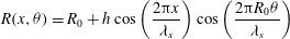 $$\begin{eqnarray}R(x,{\it\theta})=R_{0}+h\cos \left(\frac{2{\rm\pi}x}{{\it\lambda}_{x}}\right)\cos \left(\frac{2{\rm\pi}R_{0}{\it\theta}}{{\it\lambda}_{s}}\right)\end{eqnarray}$$
where
 $R_{0}$
is the reference radius of the pipe,
$R_{0}$
is the reference radius of the pipe,
 $h$
is the semi-amplitude of the sinusoidal roughness (half of the peak-to-trough height
$h$
is the semi-amplitude of the sinusoidal roughness (half of the peak-to-trough height
 $k_{t}=2h$
) and
$k_{t}=2h$
) and
 ${\it\lambda}_{x}$
and
${\it\lambda}_{x}$
and
 ${\it\lambda}_{s}$
are the wavelengths of the roughness elements in the streamwise and azimuthal directions respectively. For all of the rough cases,
${\it\lambda}_{s}$
are the wavelengths of the roughness elements in the streamwise and azimuthal directions respectively. For all of the rough cases,
 ${\it\lambda}_{x}={\it\lambda}_{s}$
. The rough-wall pipe for
${\it\lambda}_{x}={\it\lambda}_{s}$
. The rough-wall pipe for
 $h^{+}=20$
and
$h^{+}=20$
and
 ${\it\lambda}^{+}=141$
is illustrated in figure 1. In this figure, attention is drawn to four planes which embody two distinct surface characteristics:
${\it\lambda}^{+}=141$
is illustrated in figure 1. In this figure, attention is drawn to four planes which embody two distinct surface characteristics:
-
(i) The rough planes, taken through the maximum variation of roughness. These planes are labelled
 $I$
in the cross-sectional plane and
$A$
in the streamwise plane.
$I$
in the cross-sectional plane and
$A$
in the streamwise plane. -
(ii) The smooth planes, where the wall appears to be locally smooth. These planes are labelled
$II$
in the cross-sectional plane and
$B$
in the streamwise plane.


For a rough-wall pipe, the inner-scaled wall-normal direction
 $y^{+}$
is defined from the wall as
$y^{+}$
is defined from the wall as
 $$\begin{eqnarray}y^{+}=\frac{(R_{0}-r-{\it\epsilon})U_{{\it\tau}}}{{\it\nu}}\end{eqnarray}$$
where
 $r$
is the radial location measured from the centre of the pipe and
$r$
is the radial location measured from the centre of the pipe and
 ${\it\epsilon}$
the virtual origin offset due to roughness (refer to § 4.2). Throughout the paper, the roughness cases are identified by the following identifying code
${\it\epsilon}$
the virtual origin offset due to roughness (refer to § 4.2). Throughout the paper, the roughness cases are identified by the following identifying code
![]()
where the first two digits represent the roughness height and the last three digits represent the streamwise or spanwise wavelength of the roughness elements. In this paper, the roughness height
 $h^{+}$
and wavelength
$h^{+}$
and wavelength
 ${\it\lambda}^{+}$
are systematically varied to fulfil three different studies:
${\it\lambda}^{+}$
are systematically varied to fulfil three different studies:
- (C1)
-
A range of geometrically increasing roughness cases were simulated (i.e.
$h/{\it\lambda}_{x}=$
constant while
$h^{+}$
varied). The geometrically scaled case is of relevance since this is the case that is typically tested in laboratories, where the same surface is subjected to various bulk flow velocities to map out the dependence of
$C_{f}$
on the bulk Reynolds number. - (C2)
-
The wavelength of the roughness
${\it\lambda}^{+}$
is varied while maintaining the roughness height to determine the effects of wavelength alone on the roughness function (i.e.
$h^{+}=$
constant while
${\it\lambda}_{x}^{+}$
varied). - (C3)
-
The roughness height
$h^{+}$
is increased while maintaining a constant roughness wavelength to investigate the effects of roughness height in isolation from changes in wavelength (i.e.
${\it\lambda}_{x}^{+}=$
constant while
$h^{+}$
varied).


An additional range of cases is conducted to investigate the validity of the low Reynolds number simulations (cases labelled
 $\mathit{RE}$
). For this study, rough case 20\_141 (the largest rough case) and the smooth-wall pipe are simulated at
$\mathit{RE}$
). For this study, rough case 20\_141 (the largest rough case) and the smooth-wall pipe are simulated at
 $\mathit{Re}_{{\it\tau}}=180,360$
and 540. The roughness cases are partitioned into these studies in table 2. A sketch of the pipe cross-sections we have simulated through plane
$\mathit{Re}_{{\it\tau}}=180,360$
and 540. The roughness cases are partitioned into these studies in table 2. A sketch of the pipe cross-sections we have simulated through plane
 $I$
are presented by the black curves in figure 2. The corresponding cross-sections through plane
$I$
are presented by the black curves in figure 2. The corresponding cross-sections through plane
 $II$
(which are always circular) are shown by the dashed grey curves. Note that for cases 10\_283 and 02\_141, where the roughness elements have a high roughness-wavelength-to-roughness-height ratio, the walls of the pipe in plane
$II$
(which are always circular) are shown by the dashed grey curves. Note that for cases 10\_283 and 02\_141, where the roughness elements have a high roughness-wavelength-to-roughness-height ratio, the walls of the pipe in plane
 $I$
become faceted and do not appear to consist of roughness elements. Rather, the flow is passing through a deformed square/circular pipe (from plane
$I$
become faceted and do not appear to consist of roughness elements. Rather, the flow is passing through a deformed square/circular pipe (from plane
 $I$
to plane
$I$
to plane
 $II$
) for case 10\_283 and through a deformed octagonal/circular pipe for case 02\_141.
$II$
) for case 10\_283 and through a deformed octagonal/circular pipe for case 02\_141.
Table 2. Description of the different roughness elements analysed at
 $\mathit{Re}_{{\it\tau}}\approx 180,360$
and 540.
$\mathit{Re}_{{\it\tau}}\approx 180,360$
and 540.
 $h$
is the roughness mean to peak amplitude,
$h$
is the roughness mean to peak amplitude,
 ${\it\lambda}_{x}$
the roughness wavelength and
${\it\lambda}_{x}$
the roughness wavelength and
 $h/{\it\lambda}_{x}$
the aspect ratio of the roughness elements;
$h/{\it\lambda}_{x}$
the aspect ratio of the roughness elements;
 $k_{a}^{+}$
is the roughness average height,
$k_{a}^{+}$
is the roughness average height,
 $k_{rms}^{+}$
is the root-mean-square height of the roughness and
$k_{rms}^{+}$
is the root-mean-square height of the roughness and
 $\mathit{ES}$
is the effective slope of the surface. The virtual origin offsets are calculated using:
$\mathit{ES}$
is the effective slope of the surface. The virtual origin offsets are calculated using:
 ${\it\epsilon}_{1}$
, the mean momentum absorption plane method;
${\it\epsilon}_{1}$
, the mean momentum absorption plane method;
 ${\it\epsilon}_{2}$
, where
${\it\epsilon}_{2}$
, where
 $U^{+}=0$
; and
$U^{+}=0$
; and
 ${\it\epsilon}_{3}$
, where
${\it\epsilon}_{3}$
, where
 $U^{+}=1$
and then shifted by
$U^{+}=1$
and then shifted by
 $y^{+}=-1$
.
$y^{+}=-1$
.


Figure 2. Cross-sectional sketch of the roughness cases for
 $\mathit{Re}_{{\it\tau}}=180$
. Sketches in black are the cases simulated in this paper at plane I. Grey dashed lines show the simulated cases at plane II. The classification under labels C1, C2 and C3 is also shown.
$\mathit{Re}_{{\it\tau}}=180$
. Sketches in black are the cases simulated in this paper at plane I. Grey dashed lines show the simulated cases at plane II. The classification under labels C1, C2 and C3 is also shown.
Statistical parameters used to characterise the rough surface are tabulated in table 2. Increasing
 $h^{+}$
increases the roughness average height
$h^{+}$
increases the roughness average height
 $k_{a}$
, defined by ASME (2009) as the arithmetic average of the absolute values of the profile height deviations from the mean line,
$k_{a}$
, defined by ASME (2009) as the arithmetic average of the absolute values of the profile height deviations from the mean line,
 $$\begin{eqnarray}k_{a}=\frac{1}{2{\rm\pi}L_{x}}\int _{0}^{2{\rm\pi}}\int _{0}^{L_{x}}|R(x,{\it\theta})-\overline{R}|\text{d}x\text{d}{\it\theta}.\end{eqnarray}$$
For our pipe the mean line would be the reference radius of the pipe, i.e.
 $\overline{R}=R_{0}$
. The parameter
$\overline{R}=R_{0}$
. The parameter
 $k_{a}$
is one of the most common measures used in general engineering practice as it is easy to obtain. It is frequently used to analyse surface finish, where this single-value parameter makes it simple to determine if the surface has met the required standard. The value of
$k_{a}$
is one of the most common measures used in general engineering practice as it is easy to obtain. It is frequently used to analyse surface finish, where this single-value parameter makes it simple to determine if the surface has met the required standard. The value of
 $k_{a}$
, which is essentially a first-order moment of the absolute roughness height, is not as sensitive to occasional peaks on the surface compared to higher-order moments such as the root-mean-square
$k_{a}$
, which is essentially a first-order moment of the absolute roughness height, is not as sensitive to occasional peaks on the surface compared to higher-order moments such as the root-mean-square
 $k_{rms}$
(square root of the second-order moment), skewness
$k_{rms}$
(square root of the second-order moment), skewness
 $k_{sk}$
(normalised third-order moment) and kurtosis
$k_{sk}$
(normalised third-order moment) and kurtosis
 $k_{ku}$
(normalised fourth-order moment). Thus, it is unlikely that
$k_{ku}$
(normalised fourth-order moment). Thus, it is unlikely that
 $k_{a}$
alone will be sufficient to characterise the effect of a sparse rough surface on a wall-bounded flow, although Acharya, Bornstein & Escudier (Reference Acharya, Bornstein and Escudier1986) do collate
$k_{a}$
alone will be sufficient to characterise the effect of a sparse rough surface on a wall-bounded flow, although Acharya, Bornstein & Escudier (Reference Acharya, Bornstein and Escudier1986) do collate
 $k_{a}^{+}$
against
$k_{a}^{+}$
against
 ${\rm\Delta}U^{+}$
for a limited selection of roughness geometries, showing quite reasonable collapse for certain surfaces. For the current roughness geometries, constructed from simple cosines,
${\rm\Delta}U^{+}$
for a limited selection of roughness geometries, showing quite reasonable collapse for certain surfaces. For the current roughness geometries, constructed from simple cosines,
 $k_{rms}$
and
$k_{rms}$
and
 $k_{a}$
are a constant multiple of the roughness height
$k_{a}$
are a constant multiple of the roughness height
 $h$
where
$h$
where
 $h=2k_{rms}=({\rm\pi}^{2}/4)k_{a}\approx 2.46k_{a}$
, while the skewness for all the surfaces is zero. Reductions in the wavelength of the roughness elements cause an increase in the density of roughness elements per unit wall-parallel surface area. Reductions in wavelength at fixed
$h=2k_{rms}=({\rm\pi}^{2}/4)k_{a}\approx 2.46k_{a}$
, while the skewness for all the surfaces is zero. Reductions in the wavelength of the roughness elements cause an increase in the density of roughness elements per unit wall-parallel surface area. Reductions in wavelength at fixed
 $h$
also cause a steepening of the roughness, which can be characterised by the effective slope
$h$
also cause a steepening of the roughness, which can be characterised by the effective slope
 $\mathit{ES}$
(Napoli et al.
Reference Napoli, Armenio and De Marchis2008). The equation for
$\mathit{ES}$
(Napoli et al.
Reference Napoli, Armenio and De Marchis2008). The equation for
 $\mathit{ES}$
, which is the mean absolute streamwise gradient of the surface, was defined by Napoli et al. (Reference Napoli, Armenio and De Marchis2008) for two-dimensional rough surfaces. Here, this equation is generalised for three-dimensional roughnesses as
$\mathit{ES}$
, which is the mean absolute streamwise gradient of the surface, was defined by Napoli et al. (Reference Napoli, Armenio and De Marchis2008) for two-dimensional rough surfaces. Here, this equation is generalised for three-dimensional roughnesses as
 $$\begin{eqnarray}\mathit{ES}=\frac{1}{2{\rm\pi}L_{x}}\int _{0}^{2{\rm\pi}}\int _{0}^{L_{x}}\left|\frac{\partial R(x,{\it\theta})}{\partial x}\right|\text{d}x\text{d}{\it\theta}.\end{eqnarray}$$
This parameter is also related to solidity
 ${\it\Lambda}$
by the relationship
${\it\Lambda}$
by the relationship
 $\mathit{ES}=2{\it\Lambda}$
(Napoli et al.
Reference Napoli, Armenio and De Marchis2008). For inhomogeneous roughness,
$\mathit{ES}=2{\it\Lambda}$
(Napoli et al.
Reference Napoli, Armenio and De Marchis2008). For inhomogeneous roughness,
 $\mathit{ES}$
is a more general parameter which can be easily calculated with the use of a profilometer or if the equation of the surface is known. For the present sinusoidal roughness, it can be shown that
$\mathit{ES}$
is a more general parameter which can be easily calculated with the use of a profilometer or if the equation of the surface is known. For the present sinusoidal roughness, it can be shown that
 $\mathit{ES}=(8/{\rm\pi})h/{\it\lambda}_{x}$
.
$\mathit{ES}=(8/{\rm\pi})h/{\it\lambda}_{x}$
.

Figure 3. (a) Mean streamwise velocity profile for the smooth-wall pipe. Dash-dotted lines show
 $U^{+}=y^{+}$
and
$U^{+}=y^{+}$
and
 $U^{+}=(1/{\it\kappa})\log (y^{+})+C$
, where
$U^{+}=(1/{\it\kappa})\log (y^{+})+C$
, where
 ${\it\kappa}=0.40$
and
${\it\kappa}=0.40$
and
 $C=5.3$
. (b) Radial, azimuthal and streamwise components of turbulence intensity for the smooth-wall pipe. (c) Reynolds shear stress for the smooth-wall pipe. Viscous stress
$C=5.3$
. (b) Radial, azimuthal and streamwise components of turbulence intensity for the smooth-wall pipe. (c) Reynolds shear stress for the smooth-wall pipe. Viscous stress
 $-\text{d}U^{+}/\text{d}r^{+}$
and total stress of the current simulation are denoted by the dotted and dash-dotted line respectively. (d) Root-mean-squared pressure fluctuations for the smooth-wall pipe. Solid lines: second-order finite difference code at
$-\text{d}U^{+}/\text{d}r^{+}$
and total stress of the current simulation are denoted by the dotted and dash-dotted line respectively. (d) Root-mean-squared pressure fluctuations for the smooth-wall pipe. Solid lines: second-order finite difference code at
 $\mathit{Re}_{{\it\tau}}=180$
. Dashed line: spectral code at
$\mathit{Re}_{{\it\tau}}=180$
. Dashed line: spectral code at
 $\mathit{Re}_{{\it\tau}}\approx 170$
(Chin et al.
Reference Chin, Ooi, Marusic and Blackburn2010) and
$\mathit{Re}_{{\it\tau}}\approx 170$
(Chin et al.
Reference Chin, Ooi, Marusic and Blackburn2010) and
 $\mathit{Re}_{{\it\tau}}\approx 190$
(Loulou et al.
Reference Loulou, Moser, Mansour and Cantwell1997).
$\mathit{Re}_{{\it\tau}}\approx 190$
(Loulou et al.
Reference Loulou, Moser, Mansour and Cantwell1997).
4. Results and discussion
4.1. Smooth-wall validation
The accuracy of the code CDP in simulating pipe flows is first validated by comparing our results against other published DNS results for the smooth-wall case at similar Reynolds numbers. The mean velocity profile and the turbulence intensities are shown in figures 3(a) and 3(b) respectively. It can be seen that the present mean velocity profile has excellent agreement with other existing literature (both second-order and spectral codes). The velocity profiles do not fall on the high-
 $\mathit{Re}$
log law owing to the low Reynolds number of the flow. Comparing the turbulence intensities, we also obtain good agreement with data in the existing literature. The largest discrepancy (2.8 %) occurs in the comparison of the peak values of the streamwise and azimuthal turbulence intensities with those of Eggels et al. (Reference Eggels, Unger, Weiss, Westerweel, Adrian, Friedrich and Nieuwstadt1994). An explanation for this is offered by Wu & Moin (Reference Wu and Moin2008) who argue that this is due to the relatively coarse mesh and shorter domain used by Eggels et al. (Reference Eggels, Unger, Weiss, Westerweel, Adrian, Friedrich and Nieuwstadt1994). The variation from Loulou et al. (Reference Loulou, Moser, Mansour and Cantwell1997) and Chin et al. (Reference Chin, Ooi, Marusic and Blackburn2010) is likely to be due to the slightly different Reynolds numbers,
$\mathit{Re}$
log law owing to the low Reynolds number of the flow. Comparing the turbulence intensities, we also obtain good agreement with data in the existing literature. The largest discrepancy (2.8 %) occurs in the comparison of the peak values of the streamwise and azimuthal turbulence intensities with those of Eggels et al. (Reference Eggels, Unger, Weiss, Westerweel, Adrian, Friedrich and Nieuwstadt1994). An explanation for this is offered by Wu & Moin (Reference Wu and Moin2008) who argue that this is due to the relatively coarse mesh and shorter domain used by Eggels et al. (Reference Eggels, Unger, Weiss, Westerweel, Adrian, Friedrich and Nieuwstadt1994). The variation from Loulou et al. (Reference Loulou, Moser, Mansour and Cantwell1997) and Chin et al. (Reference Chin, Ooi, Marusic and Blackburn2010) is likely to be due to the slightly different Reynolds numbers,
 $\mathit{Re}_{{\it\tau}}=170$
and
$\mathit{Re}_{{\it\tau}}=170$
and
 $\mathit{Re}_{{\it\tau}}=190$
, respectively, and possibly also because of the spectral code. The Reynolds shear stress
$\mathit{Re}_{{\it\tau}}=190$
, respectively, and possibly also because of the spectral code. The Reynolds shear stress
 $\langle \overline{u_{r}^{\prime }u_{x}^{\prime }}\rangle ^{+}$
is shown in figure 3(c) as a function of wall-normal distance. The agreement with Eggels et al. (Reference Eggels, Unger, Weiss, Westerweel, Adrian, Friedrich and Nieuwstadt1994), Fukagata & Kasagi (Reference Fukagata and Kasagi2002) and Wu & Moin (Reference Wu and Moin2008) is good and the differences observed with Loulou et al. (Reference Loulou, Moser, Mansour and Cantwell1997) and Chin et al. (Reference Chin, Ooi, Marusic and Blackburn2010) are due to the different Reynolds number. Also shown in figure 3(c) are the viscous stress and the total shear stress for the current simulation. It can be seen that the total shear stress is a linear function, which gives confidence that all relevant statistics have converged. There is some variation of
$\langle \overline{u_{r}^{\prime }u_{x}^{\prime }}\rangle ^{+}$
is shown in figure 3(c) as a function of wall-normal distance. The agreement with Eggels et al. (Reference Eggels, Unger, Weiss, Westerweel, Adrian, Friedrich and Nieuwstadt1994), Fukagata & Kasagi (Reference Fukagata and Kasagi2002) and Wu & Moin (Reference Wu and Moin2008) is good and the differences observed with Loulou et al. (Reference Loulou, Moser, Mansour and Cantwell1997) and Chin et al. (Reference Chin, Ooi, Marusic and Blackburn2010) are due to the different Reynolds number. Also shown in figure 3(c) are the viscous stress and the total shear stress for the current simulation. It can be seen that the total shear stress is a linear function, which gives confidence that all relevant statistics have converged. There is some variation of
 ${p^{\prime }}_{rms}^{+}$
, present in the literature. The peak
${p^{\prime }}_{rms}^{+}$
, present in the literature. The peak
 ${p^{\prime }}_{rms}^{+}$
is found to be fairly consistently located at
${p^{\prime }}_{rms}^{+}$
is found to be fairly consistently located at
 $y^{+}=30$
; however the value ranges from 1.82 to 2.01. The present DNS results have a peak
$y^{+}=30$
; however the value ranges from 1.82 to 2.01. The present DNS results have a peak
 ${p^{\prime }}_{rms}^{+}$
of 1.95 (figure 3
d), which is closer to the values obtained by Loulou et al. (Reference Loulou, Moser, Mansour and Cantwell1997) and Wu & Moin (Reference Wu and Moin2008). Generally, the agreement with other similar simulations from the literature is good. Even with
${p^{\prime }}_{rms}^{+}$
of 1.95 (figure 3
d), which is closer to the values obtained by Loulou et al. (Reference Loulou, Moser, Mansour and Cantwell1997) and Wu & Moin (Reference Wu and Moin2008). Generally, the agreement with other similar simulations from the literature is good. Even with
 ${p^{\prime }}_{rms}^{+}$
, for which the literature exhibits substantial variation, data from the current simulation are within the reported scatter.
${p^{\prime }}_{rms}^{+}$
, for which the literature exhibits substantial variation, data from the current simulation are within the reported scatter.
4.2. Investigation of the virtual origin
Defining the virtual origin (
 $y=0$
) for a rough wall is not straightforward. For a smooth surface
$y=0$
) for a rough wall is not straightforward. For a smooth surface
 $y=0$
is easily defined as the point at which the no-slip condition acts. For a rough surface, the virtual origin depends on roughness geometry, and is typically located somewhere between the peak and trough of the rough surface. Knowledge of the virtual origin is critical for the ability to compare statistics from different surfaces. This is especially so for the current simulations where the ratio of the reference radius of the pipe
$y=0$
is easily defined as the point at which the no-slip condition acts. For a rough surface, the virtual origin depends on roughness geometry, and is typically located somewhere between the peak and trough of the rough surface. Knowledge of the virtual origin is critical for the ability to compare statistics from different surfaces. This is especially so for the current simulations where the ratio of the reference radius of the pipe
 $R_{0}$
to the roughness height
$R_{0}$
to the roughness height
 $h$
is low. However, for flows with large
$h$
is low. However, for flows with large
 $R_{0}/h$
ratios, the virtual origin offset
$R_{0}/h$
ratios, the virtual origin offset
 ${\it\epsilon}$
, which lies somewhere between the peak and trough of the roughness, only occupies a very small fraction of the boundary layer and therefore has less influence on the profiles of turbulent statistics. Typically, the only method to determine the virtual origin offset experimentally is via the modified Clauser chart method. For example, Perry & Li (Reference Perry and Li1990) link the virtual origin with the expected log-region collapse. For the present low Reynolds number DNS data, the logarithmic region is not sufficiently defined to reliably use this technique. However, we do have the option of employing the mean momentum absorption plane method to determine the virtual offset. This method was introduced by Thom (Reference Thom1971) to determine the virtual origin of a vegetation canopy. The method essentially considers the virtual origin
${\it\epsilon}$
, which lies somewhere between the peak and trough of the roughness, only occupies a very small fraction of the boundary layer and therefore has less influence on the profiles of turbulent statistics. Typically, the only method to determine the virtual origin offset experimentally is via the modified Clauser chart method. For example, Perry & Li (Reference Perry and Li1990) link the virtual origin with the expected log-region collapse. For the present low Reynolds number DNS data, the logarithmic region is not sufficiently defined to reliably use this technique. However, we do have the option of employing the mean momentum absorption plane method to determine the virtual offset. This method was introduced by Thom (Reference Thom1971) to determine the virtual origin of a vegetation canopy. The method essentially considers the virtual origin
 ${\it\epsilon}_{1}$
to be the point at which the integrated resultant force acts, and can be expressed as
${\it\epsilon}_{1}$
to be the point at which the integrated resultant force acts, and can be expressed as
 $$\begin{eqnarray}{\it\epsilon}_{1}=\left.\int _{-h}^{h}yF_{tot}(y)\text{d}y\right/\!\int _{-h}^{h}F_{tot}(y)\text{d}y\end{eqnarray}$$
where
 $F_{tot}\;(=\langle \,\overline{f}_{p}+\overline{f}_{{\it\nu}}\rangle )$
is the time and spatial (azimuthal and streamwise) average of the total drag force acting on the roughness elements due to the viscous (
$F_{tot}\;(=\langle \,\overline{f}_{p}+\overline{f}_{{\it\nu}}\rangle )$
is the time and spatial (azimuthal and streamwise) average of the total drag force acting on the roughness elements due to the viscous (
 $\overline{f}_{{\it\nu}}$
) and pressure forces (
$\overline{f}_{{\it\nu}}$
) and pressure forces (
 $\overline{f}_{p}$
). Data on the spatial distribution of the drag and the ratio between the pressure and viscous drag on the surface of rough walls are difficult to obtain experimentally but can be easily assessed when simulated numerically. Figures 4(a) and 4(b) respectively show the normalised time-averaged pressure and viscous drag acting on the roughness elements for case 20\_141 simulated at
$\overline{f}_{p}$
). Data on the spatial distribution of the drag and the ratio between the pressure and viscous drag on the surface of rough walls are difficult to obtain experimentally but can be easily assessed when simulated numerically. Figures 4(a) and 4(b) respectively show the normalised time-averaged pressure and viscous drag acting on the roughness elements for case 20\_141 simulated at
 $\mathit{Re}_{{\it\tau}}=180$
. The maximum viscous drag is located at the crest of the roughness element due to the large streamwise velocity gradient in the wall-normal direction. The location of the maximum pressure drag is located on the slope of the forward face of the roughness element. Calculating the virtual origin using this method results in a positive virtual origin offset for all roughnesses tested here (
$\mathit{Re}_{{\it\tau}}=180$
. The maximum viscous drag is located at the crest of the roughness element due to the large streamwise velocity gradient in the wall-normal direction. The location of the maximum pressure drag is located on the slope of the forward face of the roughness element. Calculating the virtual origin using this method results in a positive virtual origin offset for all roughnesses tested here (
 ${\it\epsilon}_{1}>0$
).
${\it\epsilon}_{1}>0$
).

Figure 4. Time-averaged (a) pressure
 $\overline{f}_{p}$
and (b) viscous
$\overline{f}_{p}$
and (b) viscous
 $\overline{f}_{{\it\nu}}$
drag on the surface of the roughness for case 20\_141 normalised by the total drag across the pipe
$\overline{f}_{{\it\nu}}$
drag on the surface of the roughness for case 20\_141 normalised by the total drag across the pipe
 $F_{drag}$
, where
$F_{drag}$
, where
 $F_{drag}=\sum _{y=-h}^{h}F_{tot}(y)$
. Black contour lines denote regions with positive values while white contour lines denote regions with negative values.
$F_{drag}=\sum _{y=-h}^{h}F_{tot}(y)$
. Black contour lines denote regions with positive values while white contour lines denote regions with negative values.
An alternative method which could be used to determine the virtual origin is to locate the position where the mean streamwise velocity is zero (
 $U^{+}=0$
), a condition which is satisfied by the no-slip condition at the surface of the smooth wall. The difficulty of this method is that this location is not always uniquely defined since larger roughness heights will often exhibit flow reversal in the roughness troughs, in which case multiple points satisfy this condition. The virtual origin offset obtained using this method (taking the outermost point that satisfies the condition) differs from the results from the mean momentum absorption methods, yielding a value,
$U^{+}=0$
), a condition which is satisfied by the no-slip condition at the surface of the smooth wall. The difficulty of this method is that this location is not always uniquely defined since larger roughness heights will often exhibit flow reversal in the roughness troughs, in which case multiple points satisfy this condition. The virtual origin offset obtained using this method (taking the outermost point that satisfies the condition) differs from the results from the mean momentum absorption methods, yielding a value,
 ${\it\epsilon}_{2}$
, which is always negative. A variation of this method is to find the location where
${\it\epsilon}_{2}$
, which is always negative. A variation of this method is to find the location where
 $U^{+}=1$
and then shift it by
$U^{+}=1$
and then shift it by
 $y^{+}=-1$
to obtain the offset of the virtual origin (
$y^{+}=-1$
to obtain the offset of the virtual origin (
 ${\it\epsilon}_{3}$
). The offset obtained using this method is fairly consistent for all roughness cases with values fluctuating around 0, from
${\it\epsilon}_{3}$
). The offset obtained using this method is fairly consistent for all roughness cases with values fluctuating around 0, from
 $-2.6<{\it\epsilon}_{3}^{+}<2.2$
(except for case 80\_565).
$-2.6<{\it\epsilon}_{3}^{+}<2.2$
(except for case 80\_565).
A final suggested technique to determine the virtual origin is to collapse the total stress profile outside the roughness layer regardless of whether the pipe is smooth or not. The total stress
 ${\it\tau}(r)$
across the pipe is the sum of the viscous stress
${\it\tau}(r)$
across the pipe is the sum of the viscous stress
 $-{\it\nu}\text{d}U/\text{d}r$
and the Reynolds stress
$-{\it\nu}\text{d}U/\text{d}r$
and the Reynolds stress
 $\langle \overline{u_{r}^{\prime }u_{x}^{\prime }}\rangle$
and can be expressed as
$\langle \overline{u_{r}^{\prime }u_{x}^{\prime }}\rangle$
and can be expressed as
 $$\begin{eqnarray}{\it\tau}(r)=-{\it\nu}\frac{\text{d}U}{\text{d}r}+\langle \overline{u_{r}^{\prime }u_{x}^{\prime }}\rangle =\frac{1}{2}F_{x}r\end{eqnarray}$$
where
 $F_{x}$
is defined as the streamwise driving pressure gradient, as in (2.2), and
$F_{x}$
is defined as the streamwise driving pressure gradient, as in (2.2), and
 $r$
is taken above the roughness elements. Rearranging (4.2) and dividing both sides with the radial location of the virtual origin of the pipe
$r$
is taken above the roughness elements. Rearranging (4.2) and dividing both sides with the radial location of the virtual origin of the pipe
 $R_{v}$
(currently arbitrary), we obtain
$R_{v}$
(currently arbitrary), we obtain
 $$\begin{eqnarray}\frac{{\it\tau}(r)}{R_{v}F_{x}/2}=\frac{{\it\tau}(r)}{{\it\tau}_{w}}=\frac{r}{R_{v}}\end{eqnarray}$$
where
 ${\it\tau}_{w}=F_{x}R_{v}/2$
, identified as total wall stress which is balanced by the pressure drop in the pipe. Equation (4.3) shows that
${\it\tau}_{w}=F_{x}R_{v}/2$
, identified as total wall stress which is balanced by the pressure drop in the pipe. Equation (4.3) shows that
 $R_{v}$
can be chosen arbitrarily to ensure collapse, i.e. there is no unique solution. However, if, in analogy with a smooth wall, one insists that the wall friction is defined as the drag per plan area, then a unique definition for
$R_{v}$
can be chosen arbitrarily to ensure collapse, i.e. there is no unique solution. However, if, in analogy with a smooth wall, one insists that the wall friction is defined as the drag per plan area, then a unique definition for
 $R_{v}$
emerges. To see this, consider the volume integral of the streamwise momentum equation:
$R_{v}$
emerges. To see this, consider the volume integral of the streamwise momentum equation:
 $$\begin{eqnarray}\displaystyle & \displaystyle {\it\rho}\frac{\text{d}U_{b}}{\text{d}t}={\it\rho}F_{x}V+\int _{\partial S}(-pn_{x}+{\it\nu}\boldsymbol{n}\boldsymbol{\cdot }\boldsymbol{{\rm\nabla}}u)\text{d}S={\it\rho}F_{x}V-F_{drag}=0 & \displaystyle\end{eqnarray}$$
 $$\begin{eqnarray}\displaystyle & \Rightarrow F_{x}=F_{drag}/({\it\rho}V) & \displaystyle\end{eqnarray}$$
 $n$
denotes the normal components,
$n$
denotes the normal components,
 $V$
is the volume occupied by the fluid region, which is well defined, and
$V$
is the volume occupied by the fluid region, which is well defined, and
 $\partial S$
is the corresponding surface described by the roughness geometry. We can define the hydraulic radius of the pipe to be
$\partial S$
is the corresponding surface described by the roughness geometry. We can define the hydraulic radius of the pipe to be
 $R_{h}=\sqrt{V/({\rm\pi}L_{x})}$
. Substituting the expression for
$R_{h}=\sqrt{V/({\rm\pi}L_{x})}$
. Substituting the expression for
 $F_{x}$
into the equation for
$F_{x}$
into the equation for
 ${\it\tau}_{w}$
gives
${\it\tau}_{w}$
gives  $$\begin{eqnarray}{\it\tau}_{w}=\frac{R_{v}F_{x}}{2}=\frac{R_{v}F_{drag}}{2{\it\rho}V}=\frac{R_{v}F_{drag}}{2{\it\rho}{\rm\pi}{R_{h}}^{2}L_{x}}=\frac{\overbrace{(R_{v}/R_{h})^{2}}^{\text{Constant}}F_{drag}}{{\it\rho}\underbrace{(2{\rm\pi}R_{v}L_{x})}_{\begin{array}{@{}c@{}}\text{Plan area based}\\ \text{on virtual radius}\end{array}}}.\end{eqnarray}$$
Here, to ensure that
 ${\it\tau}_{w}$
physically represents the drag acting on the wall-plan area, the virtual radius has to be equal to the hydraulic radius
${\it\tau}_{w}$
physically represents the drag acting on the wall-plan area, the virtual radius has to be equal to the hydraulic radius
 $R_{v}=R_{h}$
such that the value of the constant is 1. It can be shown that, even for the largest roughness case simulated here (
$R_{v}=R_{h}$
such that the value of the constant is 1. It can be shown that, even for the largest roughness case simulated here (
 $R_{0}/h=9$
), the reference radius of the pipe is approximately equal to the hydraulic radius of the pipe
$R_{0}/h=9$
), the reference radius of the pipe is approximately equal to the hydraulic radius of the pipe
 $R_{0}\approx R_{h}$
with 0.15 % relative difference. Therefore using the reference radius
$R_{0}\approx R_{h}$
with 0.15 % relative difference. Therefore using the reference radius
 $R_{0}$
as the location of the virtual origin is also valid (
$R_{0}$
as the location of the virtual origin is also valid (
 ${\it\epsilon}_{4}^{+}=0$
).
${\it\epsilon}_{4}^{+}=0$
).
The different methods used to obtain the virtual origin offset are tested by applying
 ${\it\epsilon}$
to the total stress, velocity defect and streamwise turbulence intensity profiles. The virtual origin offset is applied to case 20\_141 using values of
${\it\epsilon}$
to the total stress, velocity defect and streamwise turbulence intensity profiles. The virtual origin offset is applied to case 20\_141 using values of
 ${\it\epsilon}_{1}^{+}=11.7$
,
${\it\epsilon}_{1}^{+}=11.7$
,
 ${\it\epsilon}_{2}^{+}=-4.1$
and
${\it\epsilon}_{2}^{+}=-4.1$
and
 ${\it\epsilon}_{4}^{+}=0$
as illustrated in figure 5. Figure 5(a) is a plot of the total stress of the fluid. Unlike a smooth wall where the normalised total stress approaches 1 at the wall, the total shear stress of the fluid for a rough wall within the roughness elements reduces and is balanced by the pressure and viscous stress acting on the elements of the rough surface (the sum of the pressure and viscous stress acting on the elements is shown by the grey solid line on figure 5
a). Setting the virtual radius to the reference radius of the pipe, we obtain an unsurprising collapse in the total stress of the rough-wall cases with the smooth-wall case. In addition, a good collapse in the radial turbulence intensity with the smooth wall is observed almost immediately above the roughness elements for
${\it\epsilon}_{4}^{+}=0$
as illustrated in figure 5. Figure 5(a) is a plot of the total stress of the fluid. Unlike a smooth wall where the normalised total stress approaches 1 at the wall, the total shear stress of the fluid for a rough wall within the roughness elements reduces and is balanced by the pressure and viscous stress acting on the elements of the rough surface (the sum of the pressure and viscous stress acting on the elements is shown by the grey solid line on figure 5
a). Setting the virtual radius to the reference radius of the pipe, we obtain an unsurprising collapse in the total stress of the rough-wall cases with the smooth-wall case. In addition, a good collapse in the radial turbulence intensity with the smooth wall is observed almost immediately above the roughness elements for
 ${\it\epsilon}_{4}$
(figure 5
b). While a better collapse of the velocity defect is observed for
${\it\epsilon}_{4}$
(figure 5
b). While a better collapse of the velocity defect is observed for
 ${\it\epsilon}_{2}$
compared to
${\it\epsilon}_{2}$
compared to
 ${\it\epsilon}_{4}$
(figure 5
c), using
${\it\epsilon}_{4}$
(figure 5
c), using
 ${\it\epsilon}_{1}$
as the virtual origin offset does not result in a better collapse in any of the three statistics considered. Scotti (Reference Scotti2006) observed that a virtual origin determined from the mean momentum absorption plane provided a good collapse in mean statistics. It is possible that the small differences reported here between
${\it\epsilon}_{1}$
as the virtual origin offset does not result in a better collapse in any of the three statistics considered. Scotti (Reference Scotti2006) observed that a virtual origin determined from the mean momentum absorption plane provided a good collapse in mean statistics. It is possible that the small differences reported here between
 ${\it\epsilon}_{4}$
and
${\it\epsilon}_{4}$
and
 ${\it\epsilon}_{1}$
would not be easily discernible in the higher Reynolds number results presented by Scotti (Reference Scotti2006) (where the Reynolds shear stress or the total stress were also not shown).
${\it\epsilon}_{1}$
would not be easily discernible in the higher Reynolds number results presented by Scotti (Reference Scotti2006) (where the Reynolds shear stress or the total stress were also not shown).
Overall, for the cases considered here, the virtual origin offset of the pipe
 ${\it\epsilon}_{4}$
seems to offer the most consistently reliable estimate of the virtual origin for the roughness cases simulated. Good collapse in the turbulent statistics, total-stress profile and velocity defect are also obtained for all the roughness cases in the outer region of the flow when
${\it\epsilon}_{4}$
seems to offer the most consistently reliable estimate of the virtual origin for the roughness cases simulated. Good collapse in the turbulent statistics, total-stress profile and velocity defect are also obtained for all the roughness cases in the outer region of the flow when
 ${\it\epsilon}_{4}=0$
. It should, however, be noted that the analysis presented above in (4.2)–(4.6) that leads to
${\it\epsilon}_{4}=0$
. It should, however, be noted that the analysis presented above in (4.2)–(4.6) that leads to
 ${\it\epsilon}=0$
would not be true for an external boundary layer where the flow is unbounded in the wall-normal direction and the boundary layer thickness of a rough wall differs greatly from the smooth-wall case. This would suggest that the same roughness tested at the same Reynolds number in a pipe and an external boundary layer would probably exhibit different virtual origins as well as different flow close to the roughness elements. Effectively, the constrained pipe geometry would lead to more flow within the roughness canopy, compared to the boundary layer, where the flow is effectively able to ride over the roughness elements through changes in the virtual origin. For all subsequent plots, the virtual origin of the wall is defined as the reference radius of the rough-wall pipe.
${\it\epsilon}=0$
would not be true for an external boundary layer where the flow is unbounded in the wall-normal direction and the boundary layer thickness of a rough wall differs greatly from the smooth-wall case. This would suggest that the same roughness tested at the same Reynolds number in a pipe and an external boundary layer would probably exhibit different virtual origins as well as different flow close to the roughness elements. Effectively, the constrained pipe geometry would lead to more flow within the roughness canopy, compared to the boundary layer, where the flow is effectively able to ride over the roughness elements through changes in the virtual origin. For all subsequent plots, the virtual origin of the wall is defined as the reference radius of the rough-wall pipe.

Figure 5. Plot of (a) total stress normalised by the wall stress, (b) velocity defect and (c) streamwise turbulence intensity, for the smooth wall and case 20\_141 at
 $\mathit{Re}_{{\it\tau}}=180$
with virtual origin offset
$\mathit{Re}_{{\it\tau}}=180$
with virtual origin offset
 ${\it\epsilon}_{1}^{+}=11.7$
,
${\it\epsilon}_{1}^{+}=11.7$
,
 ${\it\epsilon}_{2}^{+}=-4.1$
and
${\it\epsilon}_{2}^{+}=-4.1$
and
 ${\it\epsilon}_{4}^{+}=0$
. Thick grey line in (a) is the total wall stress (viscous and pressure) of the rough surface with
${\it\epsilon}_{4}^{+}=0$
. Thick grey line in (a) is the total wall stress (viscous and pressure) of the rough surface with
 ${\it\epsilon}_{4}^{+}=0$
. Inset: zoomed in view of the boxed region.
${\it\epsilon}_{4}^{+}=0$
. Inset: zoomed in view of the boxed region.
4.3. Investigation of low Reynolds number and low ratio of reference radius to roughness height
$R_{0}/h$

In this section, we investigate the feasibility of simulating the three-dimensional sinusoidal roughness at low Reynolds number using case
 $\mathit{RE}$
. Roughness causes a downward shift in the viscous-scaled mean velocity profile, which is typically expressed as a modified logarithmic law,
$\mathit{RE}$
. Roughness causes a downward shift in the viscous-scaled mean velocity profile, which is typically expressed as a modified logarithmic law,
 $$\begin{eqnarray}U^{+}=\frac{1}{{\it\kappa}}\ln (y^{+})+C-{\rm\Delta}U^{+},\end{eqnarray}$$
where
 ${\rm\Delta}U^{+}$
is known as the Hama roughness function (Hama Reference Hama1954). To determine if the roughness function
${\rm\Delta}U^{+}$
is known as the Hama roughness function (Hama Reference Hama1954). To determine if the roughness function
 ${\rm\Delta}U^{+}$
obtained in the low Reynolds number simulations is applicable to flows at higher Reynolds number, case 20\_141 (the case with the largest roughness) is simulated at three different Reynolds numbers (
${\rm\Delta}U^{+}$
obtained in the low Reynolds number simulations is applicable to flows at higher Reynolds number, case 20\_141 (the case with the largest roughness) is simulated at three different Reynolds numbers (
 $\mathit{Re}_{{\it\tau}}=180,360$
and 540). In this study, where Townsend’s outer-layer similarity (Townsend Reference Townsend1980) seems to be conserved (see §§ 4.5 and 4.4.5),
$\mathit{Re}_{{\it\tau}}=180,360$
and 540). In this study, where Townsend’s outer-layer similarity (Townsend Reference Townsend1980) seems to be conserved (see §§ 4.5 and 4.4.5),
 ${\rm\Delta}U^{+}$
is determined 50 wall units above the crest of the roughness elements for all of the cases simulated since the log layer of the flow at low and moderate Reynolds numbers is poorly defined. As the roughness elements have the same viscous scale, the physical geometrical size of the roughness element relative to the pipe radius reduces with increasing Reynolds number. The sketches of the rough pipe in figure 6 clearly illustrates this where
${\rm\Delta}U^{+}$
is determined 50 wall units above the crest of the roughness elements for all of the cases simulated since the log layer of the flow at low and moderate Reynolds numbers is poorly defined. As the roughness elements have the same viscous scale, the physical geometrical size of the roughness element relative to the pipe radius reduces with increasing Reynolds number. The sketches of the rough pipe in figure 6 clearly illustrates this where
 $R_{0}/h$
increases from 9 at
$R_{0}/h$
increases from 9 at
 $\mathit{Re}_{{\it\tau}}=180$
to 27 when
$\mathit{Re}_{{\it\tau}}=180$
to 27 when
 $\mathit{Re}_{{\it\tau}}=540$
. Hence, these experiments also address the influence of
$\mathit{Re}_{{\it\tau}}=540$
. Hence, these experiments also address the influence of
 $R_{0}/h$
for this particular roughness.
$R_{0}/h$
for this particular roughness.

Figure 6. Streamwise velocity profile for smooth wall and case 20\_141 at
 $\mathit{Re}_{{\it\tau}}=180,360$
and 540. Dash-dotted lines show
$\mathit{Re}_{{\it\tau}}=180,360$
and 540. Dash-dotted lines show
 $U^{+}=y^{+}$
and
$U^{+}=y^{+}$
and
 $U^{+}=(1/{\it\kappa})\log (y^{+})+C$
,
$U^{+}=(1/{\it\kappa})\log (y^{+})+C$
,
 ${\it\kappa}=0.40$
and
${\it\kappa}=0.40$
and
 $C=5.3$
. Inset: roughness function
$C=5.3$
. Inset: roughness function
 ${\rm\Delta}U^{+}$
against
${\rm\Delta}U^{+}$
against
 $y^{+}$
for the different Reynolds number simulation. Note that
$y^{+}$
for the different Reynolds number simulation. Note that
 $R_{0}/h$
ranges from 9 for the
$R_{0}/h$
ranges from 9 for the
 $\mathit{Re}_{{\it\tau}}=180$
simulation to 27 for the
$\mathit{Re}_{{\it\tau}}=180$
simulation to 27 for the
 $\mathit{Re}_{{\it\tau}}=540$
simulation. Refer to table 1 for symbol key.
$\mathit{Re}_{{\it\tau}}=540$
simulation. Refer to table 1 for symbol key.
Examining the mean velocity profiles for the smooth wall in figure 6, the low Reynolds number effect at
 $\mathit{Re}_{{\it\tau}}=180$
is apparent, causing an upward shift from the logarithmic region (shown by the dot–dashed line for
$\mathit{Re}_{{\it\tau}}=180$
is apparent, causing an upward shift from the logarithmic region (shown by the dot–dashed line for
 ${\it\kappa}=0.4$
and
${\it\kappa}=0.4$
and
 $C=5.3$
). This is the well-documented pressure gradient effect of low Reynolds number turbulent pipe flow (see for example Nickels Reference Nickels2004). However, for the rough cases, a closer collapse is obtained for the mean velocity profile simulated at all three Reynolds numbers. Although the low Reynolds number effect is still observable for case 20\_141 at
$C=5.3$
). This is the well-documented pressure gradient effect of low Reynolds number turbulent pipe flow (see for example Nickels Reference Nickels2004). However, for the rough cases, a closer collapse is obtained for the mean velocity profile simulated at all three Reynolds numbers. Although the low Reynolds number effect is still observable for case 20\_141 at
 $\mathit{Re}_{{\it\tau}}=180$
, it is not as significant as for the smooth wall simulated at the same Reynolds number. Calculating the difference in the mean velocity profile between the smooth and rough cases at the same Reynolds number (inset of figure 6), we observe that the profiles remain fairly constant above the roughness elements, particularly so above
$\mathit{Re}_{{\it\tau}}=180$
, it is not as significant as for the smooth wall simulated at the same Reynolds number. Calculating the difference in the mean velocity profile between the smooth and rough cases at the same Reynolds number (inset of figure 6), we observe that the profiles remain fairly constant above the roughness elements, particularly so above
 $y^{+}=70$
, indicating that the shape of the mean velocity profile in the outer part of the flow for both the smooth and rough cases is similar. Due to the low Reynolds number effect of the smooth pipe at
$y^{+}=70$
, indicating that the shape of the mean velocity profile in the outer part of the flow for both the smooth and rough cases is similar. Due to the low Reynolds number effect of the smooth pipe at
 $\mathit{Re}_{{\it\tau}}=180$
, the roughness function
$\mathit{Re}_{{\it\tau}}=180$
, the roughness function
 ${\rm\Delta}U^{+}$
is slightly overestimated. However, the maximum difference obtained in
${\rm\Delta}U^{+}$
is slightly overestimated. However, the maximum difference obtained in
 ${\rm\Delta}U^{+}$
between the
${\rm\Delta}U^{+}$
between the
 $\mathit{Re}_{{\it\tau}}=180$
and 540 simulation is only approximately 0.7. This error can be relatively insignificant in high Reynolds number flows which are of engineering interest.
$\mathit{Re}_{{\it\tau}}=180$
and 540 simulation is only approximately 0.7. This error can be relatively insignificant in high Reynolds number flows which are of engineering interest.
An overestimation of
 ${\rm\Delta}U^{+}$
by some amount
${\rm\Delta}U^{+}$
by some amount
 ${\it\varepsilon}$
, causes an overestimation of
${\it\varepsilon}$
, causes an overestimation of
 $k_{s}$
for a surface by approximately
$k_{s}$
for a surface by approximately
 $\exp ({\it\kappa}{\it\varepsilon})$
, which is approximately 33 % when
$\exp ({\it\kappa}{\it\varepsilon})$
, which is approximately 33 % when
 ${\it\varepsilon}=0.7$
. For full-scale moderate to high Reynolds number flows in the fully rough regime, this translates to an overestimation of the total drag coefficient by only approximately 5 %. Such an error is rather insignificant when one considers the traditional error associated with determining
${\it\varepsilon}=0.7$
. For full-scale moderate to high Reynolds number flows in the fully rough regime, this translates to an overestimation of the total drag coefficient by only approximately 5 %. Such an error is rather insignificant when one considers the traditional error associated with determining
 $C_{f}$
experimentally, and also that a fully rough surface can lead to
$C_{f}$
experimentally, and also that a fully rough surface can lead to
 $O(100\,\%)$
increases in drag coefficient. More important for the current simulations is that the low Reynolds number simulations are able to capture the correct trends in
$O(100\,\%)$
increases in drag coefficient. More important for the current simulations is that the low Reynolds number simulations are able to capture the correct trends in
 ${\rm\Delta}U^{+}$
with varying roughness geometry. This is confirmed for the case of varying effective slope in figure 10 below. An improved method which could be used to obtain a more accurate value of
${\rm\Delta}U^{+}$
with varying roughness geometry. This is confirmed for the case of varying effective slope in figure 10 below. An improved method which could be used to obtain a more accurate value of
 ${\rm\Delta}U^{+}$
for large roughnesses simulated at low
${\rm\Delta}U^{+}$
for large roughnesses simulated at low
 $\mathit{Re}_{{\it\tau}}$
would be to calculate the shift in the log-law from a higher Reynolds number smooth-wall simulation.
$\mathit{Re}_{{\it\tau}}$
would be to calculate the shift in the log-law from a higher Reynolds number smooth-wall simulation.
For the transitional roughness cases which have been simulated, the observance of outer-layer similarity in the outer part of the flow appears to be insensitive to changes in the
 $R_{0}/h$
ratio. The total stress profiles of the smooth and rough cases are shown in figure 7(a), and as expected show an excellent collapse for all the cases when the virtual origin is set to be the reference radius of the pipe. In addition, very good collapse is observed in the radial turbulence intensity between the smooth and rough cases as illustrated in figure 7(c). Reasonable collapse is also obtained when the mean velocity profile is plotted in defect form in figure 7(b), with no pronounced difference in this collapse with varying
$R_{0}/h$
ratio. The total stress profiles of the smooth and rough cases are shown in figure 7(a), and as expected show an excellent collapse for all the cases when the virtual origin is set to be the reference radius of the pipe. In addition, very good collapse is observed in the radial turbulence intensity between the smooth and rough cases as illustrated in figure 7(c). Reasonable collapse is also obtained when the mean velocity profile is plotted in defect form in figure 7(b), with no pronounced difference in this collapse with varying
 $R_{0}/h$
. Overall, the adherence to Townsend’s outer-layer similarity of the mean statistics for the rough cases is invariant with Reynolds number and hence also with the ratio
$R_{0}/h$
. Overall, the adherence to Townsend’s outer-layer similarity of the mean statistics for the rough cases is invariant with Reynolds number and hence also with the ratio
 $R_{0}/h$
.
$R_{0}/h$
.

Figure 7. (a) Total stress normalised by the wall stress; (b) velocity defect; and (c) radial turbulence intensity for the smooth wall and case 20\_141 at
 $\mathit{Re}_{{\it\tau}}=180,360$
and 540.
$\mathit{Re}_{{\it\tau}}=180,360$
and 540.
Based on these observations, the decision was made to run the majority of our simulations at
 $\mathit{Re}_{{\it\tau}}=180$
. Although
$\mathit{Re}_{{\it\tau}}=180$
. Although
 $\mathit{Re}_{{\it\tau}}=360$
would give a slightly more accurate representation of
$\mathit{Re}_{{\it\tau}}=360$
would give a slightly more accurate representation of
 ${\rm\Delta}U^{+}$
(by avoiding the low Reynolds number pressure gradient effect), these simulations are approximately eight times more expensive. In this instance, we believe that the contribution from this study would be maximised by testing an increased number of surface geometries and thus we choose to deploy our computational resources in this manner. However, throughout this study, certain surfaces will also be computed at
${\rm\Delta}U^{+}$
(by avoiding the low Reynolds number pressure gradient effect), these simulations are approximately eight times more expensive. In this instance, we believe that the contribution from this study would be maximised by testing an increased number of surface geometries and thus we choose to deploy our computational resources in this manner. However, throughout this study, certain surfaces will also be computed at
 $\mathit{Re}_{{\it\tau}}=360$
, to continually verify that the important results and trends observed in this study are not artifacts of low
$\mathit{Re}_{{\it\tau}}=360$
, to continually verify that the important results and trends observed in this study are not artifacts of low
 $\mathit{Re}$
or low
$\mathit{Re}$
or low
 $R_{0}/h$
.
$R_{0}/h$
.
4.4. Mean velocity profiles
4.4.1. Case C1: geometrically scaled roughness (fixed
${\it\lambda}/h$
)

The mean streamwise velocity profile for the geometrically scaled roughness cases (C1) are plotted in figure 8 for the cases simulated at
 $\mathit{Re}_{{\it\tau}}=180$
and figure 9 for the cases simulated at
$\mathit{Re}_{{\it\tau}}=180$
and figure 9 for the cases simulated at
 $\mathit{Re}_{{\it\tau}}=540$
. Geometrically increasing the size of the roughness increases the roughness average height, with proportionate increases in
$\mathit{Re}_{{\it\tau}}=540$
. Geometrically increasing the size of the roughness increases the roughness average height, with proportionate increases in
 ${\it\lambda}_{x}$
and
${\it\lambda}_{x}$
and
 ${\it\lambda}_{s}$
. The aspect ratio and average slope of the surface (and hence
${\it\lambda}_{s}$
. The aspect ratio and average slope of the surface (and hence
 $\mathit{ES}$
) remains unchanged. An increase in the geometric scaling factor yields an increase in the roughness function as observed in the insets of figures 8 and 9. It is important to highlight that for cases 02\_018 and 05\_035, there are only four and eight grid points per roughness wavelength and hence the topological features of the sinusoidal surface are not fully resolved (a more faceted version of the roughness is effectively simulated). Thus, this may result in some minor discrepancies in the obtained
$\mathit{ES}$
) remains unchanged. An increase in the geometric scaling factor yields an increase in the roughness function as observed in the insets of figures 8 and 9. It is important to highlight that for cases 02\_018 and 05\_035, there are only four and eight grid points per roughness wavelength and hence the topological features of the sinusoidal surface are not fully resolved (a more faceted version of the roughness is effectively simulated). Thus, this may result in some minor discrepancies in the obtained
 ${\rm\Delta}U^{+}$
(which can be confirmed by conducting a grid sensitivity analysis).
${\rm\Delta}U^{+}$
(which can be confirmed by conducting a grid sensitivity analysis).

Figure 8. Streamwise velocity profile for geometrically scaled roughness cases at
 $\mathit{Re}_{{\it\tau}}=180$
. Dash-dotted lines show
$\mathit{Re}_{{\it\tau}}=180$
. Dash-dotted lines show
 $U^{+}=y^{+}$
and
$U^{+}=y^{+}$
and
 $U^{+}=(1/{\it\kappa})\log (y^{+})+C$
,
$U^{+}=(1/{\it\kappa})\log (y^{+})+C$
,
 ${\it\kappa}=0.40$
and
${\it\kappa}=0.40$
and
 $C=5.3$
. Inset: roughness function
$C=5.3$
. Inset: roughness function
 ${\rm\Delta}U^{+}$
against roughness height
${\rm\Delta}U^{+}$
against roughness height
 $h^{+}$
. Dash-dotted line of the inset flow demarcates the fully rough asymptote where
$h^{+}$
. Dash-dotted line of the inset flow demarcates the fully rough asymptote where
 $k_{s}^{+}=4.1h^{+}$
.
$k_{s}^{+}=4.1h^{+}$
.

Figure 9. Streamwise velocity profile for geometrically scaled roughness cases at
 $\mathit{Re}_{{\it\tau}}=540$
. Dash-dotted lines show
$\mathit{Re}_{{\it\tau}}=540$
. Dash-dotted lines show
 $U^{+}=y^{+}$
and
$U^{+}=y^{+}$
and
 $U^{+}=(1/{\it\kappa})\log (y^{+})+C$
,
$U^{+}=(1/{\it\kappa})\log (y^{+})+C$
,
 ${\it\kappa}=0.40$
and
${\it\kappa}=0.40$
and
 $C=5.3$
. Inset: roughness function
$C=5.3$
. Inset: roughness function
 ${\rm\Delta}U^{+}$
against roughness height
${\rm\Delta}U^{+}$
against roughness height
 $h^{+}$
. Dash-dotted line of the inset flow demarcates the fully rough asymptote where
$h^{+}$
. Dash-dotted line of the inset flow demarcates the fully rough asymptote where
 $k_{s}^{+}=4.1h^{+}$
. Refer to table 1 for symbol key.
$k_{s}^{+}=4.1h^{+}$
. Refer to table 1 for symbol key.
It appears that the flow reaches the fully rough regime when
 $h^{+}\approx 60$
which corresponds to an equivalent sand grain roughness of
$h^{+}\approx 60$
which corresponds to an equivalent sand grain roughness of
 $k_{s}^{+}=4.1h^{+}$
. Hence this dataset spans the full transitional regime, from smooth up to fully rough. To the best of the authors’ knowledge this is the first time that
$k_{s}^{+}=4.1h^{+}$
. Hence this dataset spans the full transitional regime, from smooth up to fully rough. To the best of the authors’ knowledge this is the first time that
 $k_{s}^{+}$
verses
$k_{s}^{+}$
verses
 ${\rm\Delta}U^{+}$
has been mapped from smooth up to the fully rough regime using DNS with a body-conforming grid.
${\rm\Delta}U^{+}$
has been mapped from smooth up to the fully rough regime using DNS with a body-conforming grid.
4.4.2. Case C2: decreasing roughness wavelength
${\it\lambda}^{+}$
(fixed
$h^{+}=10$
)


Figure 10 shows mean streamwise velocity profiles for the cases where the wavelength of the roughness elements is varied while maintaining a constant roughness height (case C2). Decreasing the wavelength of the roughness elements increases the
 $\mathit{ES}$
of the surface and allows us to analyse the effects of
$\mathit{ES}$
of the surface and allows us to analyse the effects of
 $\mathit{ES}$
on the roughness function independently of roughness height. In addition, the roughness elements become ‘more dense’ with decreasing wavelength (increased solidity
$\mathit{ES}$
on the roughness function independently of roughness height. In addition, the roughness elements become ‘more dense’ with decreasing wavelength (increased solidity
 ${\it\Lambda}$
). Despite reducing the wavelength of the roughness elements by about a quarter (four times the number of roughness elements), there was only an increase of
${\it\Lambda}$
). Despite reducing the wavelength of the roughness elements by about a quarter (four times the number of roughness elements), there was only an increase of
 ${\approx}1.56$
in
${\approx}1.56$
in
 ${\rm\Delta}U^{+}$
between case 10\_283 and 10\_070. The very gradual increase in the roughness function observed in the inset of figure 10 when the roughness wavelength decreases suggests that
${\rm\Delta}U^{+}$
between case 10\_283 and 10\_070. The very gradual increase in the roughness function observed in the inset of figure 10 when the roughness wavelength decreases suggests that
 $\mathit{ES}$
has only a secondary importance in the flow compared to the average roughness height for the current surface geometry in the transitionally rough regime. It is interesting to consider the asymptotic limits that we might expect for variations in
$\mathit{ES}$
has only a secondary importance in the flow compared to the average roughness height for the current surface geometry in the transitionally rough regime. It is interesting to consider the asymptotic limits that we might expect for variations in
 ${\it\lambda}$
. When
${\it\lambda}$
. When
 ${\it\lambda}\rightarrow \infty$
we would expect the surface to approach the smooth case. We might expect a similar behaviour as
${\it\lambda}\rightarrow \infty$
we would expect the surface to approach the smooth case. We might expect a similar behaviour as
 ${\it\lambda}\rightarrow 0$
(although with this case, the pipe radius will be altered). Selected duplicated cases were simulated at
${\it\lambda}\rightarrow 0$
(although with this case, the pipe radius will be altered). Selected duplicated cases were simulated at
 $\mathit{Re}_{{\it\tau}}=360$
(circled symbols) and a similar trend is observed with varying wavelength, further assuaging any doubts that the low
$\mathit{Re}_{{\it\tau}}=360$
(circled symbols) and a similar trend is observed with varying wavelength, further assuaging any doubts that the low
 $\mathit{Re}$
(and low
$\mathit{Re}$
(and low
 $R_{0}/h$
) of these simulations is influencing observed trends.
$R_{0}/h$
) of these simulations is influencing observed trends.

Figure 10. Streamwise velocity profile for cases with decreasing roughness wavelength
 ${\it\lambda}^{+}$
. Dash-dotted lines show
${\it\lambda}^{+}$
. Dash-dotted lines show
 $U^{+}=y^{+}$
and
$U^{+}=y^{+}$
and
 $U^{+}=(1/{\it\kappa})\log \!(y^{+})+C$
, where
$U^{+}=(1/{\it\kappa})\log \!(y^{+})+C$
, where
 ${\it\kappa}=0.40$
and
${\it\kappa}=0.40$
and
 $C=5.3$
. Inset: roughness function
$C=5.3$
. Inset: roughness function
 ${\rm\Delta}U^{+}$
against roughness wavelength
${\rm\Delta}U^{+}$
against roughness wavelength
 ${\it\lambda}^{+}$
. Circled symbols in shades of red are simulated at
${\it\lambda}^{+}$
. Circled symbols in shades of red are simulated at
 $\mathit{Re}_{{\it\tau}}=360$
. Refer to table 1 for symbol key.
$\mathit{Re}_{{\it\tau}}=360$
. Refer to table 1 for symbol key.
4.4.3. Case C3: increasing roughness height
$h^{+}$
(fixed
${\it\lambda}^{+}=141$
)


Figure 11 plots the mean streamwise velocity profile for the cases where roughness height is increased while the wavelength remains fixed (case C3). This yields increasing aspect ratio (and increasing
 $\mathit{ES}$
) as
$\mathit{ES}$
) as
 $h$
increases. Not surprisingly, increasing
$h$
increases. Not surprisingly, increasing
 $h^{+}$
leads to increments in
$h^{+}$
leads to increments in
 ${\rm\Delta}U^{+}$
. Comparing the inset of figure 11 with figure 9 shows that the geometrically scaled surfaces (case C1) yield a much higher
${\rm\Delta}U^{+}$
. Comparing the inset of figure 11 with figure 9 shows that the geometrically scaled surfaces (case C1) yield a much higher
 ${\rm\Delta}U^{+}$
at low
${\rm\Delta}U^{+}$
at low
 $h^{+}$
than the fixed wavelength case C3. This is an expected result from figure 10, since the geometrically scaled cases have a higher value of effective slope, and therefore a higher
$h^{+}$
than the fixed wavelength case C3. This is an expected result from figure 10, since the geometrically scaled cases have a higher value of effective slope, and therefore a higher
 ${\rm\Delta}U^{+}$
, than the C3 cases at low
${\rm\Delta}U^{+}$
, than the C3 cases at low
 $h^{+}$
.
$h^{+}$
.

Figure 11. Streamwise velocity profile for cases with increasing roughness height
 $h^{+}$
. Dash-dotted lines show
$h^{+}$
. Dash-dotted lines show
 $U^{+}=y^{+}$
and
$U^{+}=y^{+}$
and
 $U^{+}=(1/{\it\kappa})\log (y^{+})+C$
, where
$U^{+}=(1/{\it\kappa})\log (y^{+})+C$
, where
 ${\it\kappa}=0.40$
and
${\it\kappa}=0.40$
and
 $C=5.3$
. Inset: roughness function
$C=5.3$
. Inset: roughness function
 ${\rm\Delta}U^{+}$
against roughness height
${\rm\Delta}U^{+}$
against roughness height
 $h^{+}$
. Circled symbols and dotted symbols show the same cases simulated at
$h^{+}$
. Circled symbols and dotted symbols show the same cases simulated at
 $\mathit{Re}_{{\it\tau}}=360$
and 540 respectively (refer to table 1 for symbol key).
$\mathit{Re}_{{\it\tau}}=360$
and 540 respectively (refer to table 1 for symbol key).
4.4.4. Consolidated mean velocity results
Figures 10 and 11 show that increasing the roughness height
 $h^{+}$
(with fixed
$h^{+}$
(with fixed
 ${\it\lambda}$
) or decreasing the wavelength of the roughness
${\it\lambda}$
) or decreasing the wavelength of the roughness
 ${\it\lambda}^{+}$
(with fixed
${\it\lambda}^{+}$
(with fixed
 $h$
) both lead to an increase in
$h$
) both lead to an increase in
 ${\rm\Delta}U^{+}$
. Both of these experiments are varying the
${\rm\Delta}U^{+}$
. Both of these experiments are varying the
 $\mathit{ES}$
of the surface. On figure 12 we further investigate these data, showing
$\mathit{ES}$
of the surface. On figure 12 we further investigate these data, showing
 ${\rm\Delta}U^{+}$
as a function of
${\rm\Delta}U^{+}$
as a function of
 $\mathit{ES}$
in plot (a) and as a function of
$\mathit{ES}$
in plot (a) and as a function of
 $k_{a}^{+}$
(which is proportional to
$k_{a}^{+}$
(which is proportional to
 $h^{+}$
) in plot (b). Additional data from Blackburn et al. (Reference Blackburn, Ooi and Chong2007) (corrugated pipe,
$h^{+}$
) in plot (b). Additional data from Blackburn et al. (Reference Blackburn, Ooi and Chong2007) (corrugated pipe,
 $\mathit{Re}_{{\it\tau}}=314$
), De Marchis & Napoli (Reference De Marchis and Napoli2012) (2D and 3D inhomogeneous rough channel,
$\mathit{Re}_{{\it\tau}}=314$
), De Marchis & Napoli (Reference De Marchis and Napoli2012) (2D and 3D inhomogeneous rough channel,
 $\mathit{Re}_{{\it\tau}}=395$
), Napoli et al. (Reference Napoli, Armenio and De Marchis2008) (2D inhomogeneous rough channel,
$\mathit{Re}_{{\it\tau}}=395$
), Napoli et al. (Reference Napoli, Armenio and De Marchis2008) (2D inhomogeneous rough channel,
 $\mathit{Re}_{{\it\tau}}=395$
), Bhaganagar, Kim & Coleman (Reference Bhaganagar, Kim and Coleman2004) (‘egg-carton’ asymmetric rough channel,
$\mathit{Re}_{{\it\tau}}=395$
), Bhaganagar, Kim & Coleman (Reference Bhaganagar, Kim and Coleman2004) (‘egg-carton’ asymmetric rough channel,
 $\mathit{Re}_{{\it\tau}}=400$
) and Schultz & Flack (Reference Schultz and Flack2009) (close-packed pyramids) are also included in the plots for a more comprehensive comparison. A horizontal line at
$\mathit{Re}_{{\it\tau}}=400$
) and Schultz & Flack (Reference Schultz and Flack2009) (close-packed pyramids) are also included in the plots for a more comprehensive comparison. A horizontal line at
 ${\rm\Delta}U^{+}=9$
is added to mark the approximate start of the fully rough regime.
${\rm\Delta}U^{+}=9$
is added to mark the approximate start of the fully rough regime.

Figure 12.
 ${\rm\Delta}U^{+}$
as a function of (a)
${\rm\Delta}U^{+}$
as a function of (a)
 $\mathit{ES}$
; (b)
$\mathit{ES}$
; (b)
 $k_{a}^{+}$
. The horizontal dashed line at
$k_{a}^{+}$
. The horizontal dashed line at
 ${\rm\Delta}U^{+}=9$
demarcates the start of the fully rough regime. Solid coloured symbols show results of the current study (symbols as defined in table 1). Light shaded symbols show results from the literature
${\rm\Delta}U^{+}=9$
demarcates the start of the fully rough regime. Solid coloured symbols show results of the current study (symbols as defined in table 1). Light shaded symbols show results from the literature
 $\otimes$
:
$\otimes$
:
 $\oplus$
,
$\oplus$
,
 $\odot$
, close-packed pyramids of Schultz & Flack (Reference Schultz and Flack2009) (for
$\odot$
, close-packed pyramids of Schultz & Flack (Reference Schultz and Flack2009) (for
 $\mathit{ES}=0.19$
, 0.4 and 1 respectively);
$\mathit{ES}=0.19$
, 0.4 and 1 respectively);
 $\times$
, ‘egg-carton’ roughness of Bhaganagar et al. (Reference Bhaganagar, Kim and Coleman2004);
$\times$
, ‘egg-carton’ roughness of Bhaganagar et al. (Reference Bhaganagar, Kim and Coleman2004);
 $\ast$
, 2D and 3D inhomogeneous roughness of De Marchis & Napoli (Reference De Marchis and Napoli2012);
$\ast$
, 2D and 3D inhomogeneous roughness of De Marchis & Napoli (Reference De Marchis and Napoli2012);
 $\boxdot$
, corrugated pipe of Blackburn et al. (Reference Blackburn, Ooi and Chong2007); ♢, 2D inhomogeneous roughness of Napoli et al. (Reference Napoli, Armenio and De Marchis2008).
$\boxdot$
, corrugated pipe of Blackburn et al. (Reference Blackburn, Ooi and Chong2007); ♢, 2D inhomogeneous roughness of Napoli et al. (Reference Napoli, Armenio and De Marchis2008).
In figure 12(a), it is clearly observed that
 ${\rm\Delta}U^{+}$
does not scale solely with
${\rm\Delta}U^{+}$
does not scale solely with
 $\mathit{ES}$
. This is especially true for data obtained by Schultz & Flack (Reference Schultz and Flack2009) where the same rough surfaces were tested at various Reynolds numbers, thus changing the value of
$\mathit{ES}$
. This is especially true for data obtained by Schultz & Flack (Reference Schultz and Flack2009) where the same rough surfaces were tested at various Reynolds numbers, thus changing the value of
 $k_{a}^{+}$
while maintaining constant
$k_{a}^{+}$
while maintaining constant
 $\mathit{ES}$
. It is clearly visible in their data that
$\mathit{ES}$
. It is clearly visible in their data that
 ${\rm\Delta}U^{+}$
increases as
${\rm\Delta}U^{+}$
increases as
 $k_{a}^{+}$
increases for a given
$k_{a}^{+}$
increases for a given
 $\mathit{ES}$
. Our current simulations, which are mostly in the transitionally rough regime, also do not collapse onto the trend reported by Napoli et al. (Reference Napoli, Armenio and De Marchis2008) (♢ symbols). Yuan & Piomelli (Reference Yuan and Piomelli2014) also did not find a collapse onto the curve given by Napoli et al. (Reference Napoli, Armenio and De Marchis2008), observing that the plateau in
$\mathit{ES}$
. Our current simulations, which are mostly in the transitionally rough regime, also do not collapse onto the trend reported by Napoli et al. (Reference Napoli, Armenio and De Marchis2008) (♢ symbols). Yuan & Piomelli (Reference Yuan and Piomelli2014) also did not find a collapse onto the curve given by Napoli et al. (Reference Napoli, Armenio and De Marchis2008), observing that the plateau in
 $\mathit{ES}$
versus
$\mathit{ES}$
versus
 ${\rm\Delta}U^{+}$
can occur at larger values of
${\rm\Delta}U^{+}$
can occur at larger values of
 $\mathit{ES}$
for different surfaces. In figure 12(b), we plot
$\mathit{ES}$
for different surfaces. In figure 12(b), we plot
 ${\rm\Delta}U^{+}$
against
${\rm\Delta}U^{+}$
against
 $k_{a}^{+}$
, which in §§ 4.4.1 and 4.4.3 were found to be strongly correlated. When scaled in this manner, a reasonable collapse in the data is observed in the fully rough regime as the roughness function follows a log function of
$k_{a}^{+}$
, which in §§ 4.4.1 and 4.4.3 were found to be strongly correlated. When scaled in this manner, a reasonable collapse in the data is observed in the fully rough regime as the roughness function follows a log function of
 ${\rm\Delta}U^{+}=(1/{\it\kappa})\log (C_{eq}k_{a}^{+})+5.3-8.5$
, where
${\rm\Delta}U^{+}=(1/{\it\kappa})\log (C_{eq}k_{a}^{+})+5.3-8.5$
, where
 $C_{eq}$
is the multiplicative factor for the roughness function to fall on to the fully rough asymptote of the sand grain roughness. However, there is still considerable scatter in the data, notably in the transitionally rough regime. Cases with low effective slope (
$C_{eq}$
is the multiplicative factor for the roughness function to fall on to the fully rough asymptote of the sand grain roughness. However, there is still considerable scatter in the data, notably in the transitionally rough regime. Cases with low effective slope (
 $\mathit{ES}<0.2$
), do not appear to approach the fully rough regime and contribute to the scatter. Obvious outliers are the pyramid data from Schultz & Flack (Reference Schultz and Flack2009) for the cases when
$\mathit{ES}<0.2$
), do not appear to approach the fully rough regime and contribute to the scatter. Obvious outliers are the pyramid data from Schultz & Flack (Reference Schultz and Flack2009) for the cases when
 $\mathit{ES}=0.19$
(
$\mathit{ES}=0.19$
(
 $\otimes$
symbols). The small gradients of these close-packed pyramids resemble more a gently undulating (‘wavy’) surface rather than a sawtooth roughness, thus indicating that
$\otimes$
symbols). The small gradients of these close-packed pyramids resemble more a gently undulating (‘wavy’) surface rather than a sawtooth roughness, thus indicating that
 $\mathit{ES}$
has a significant role in determining the asymptotic behaviour of the rough surface (e.g. if it approaches the fully rough regime). This is also observed in the experiments conducted by Acharya et al. (Reference Acharya, Bornstein and Escudier1986) where the
$\mathit{ES}$
has a significant role in determining the asymptotic behaviour of the rough surface (e.g. if it approaches the fully rough regime). This is also observed in the experiments conducted by Acharya et al. (Reference Acharya, Bornstein and Escudier1986) where the
 ${\rm\Delta}U^{+}$
profile does not have the same slope as the fully rough sand grain roughnesses for the tested surface with the largest
${\rm\Delta}U^{+}$
profile does not have the same slope as the fully rough sand grain roughnesses for the tested surface with the largest
 ${\it\lambda}/k_{a}$
ratio, which might be in the ‘wavy’ regime. Results from their experimental data also appear to suggest that the multiplicative factor
${\it\lambda}/k_{a}$
ratio, which might be in the ‘wavy’ regime. Results from their experimental data also appear to suggest that the multiplicative factor
 $C_{eq}$
might depend on
$C_{eq}$
might depend on
 $\mathit{ES}$
. In addition, the study of Napoli et al. (Reference Napoli, Armenio and De Marchis2008) clearly demonstrates that
$\mathit{ES}$
. In addition, the study of Napoli et al. (Reference Napoli, Armenio and De Marchis2008) clearly demonstrates that
 $\mathit{ES}$
is an important parameter. They simulated six different roughnesses with the same
$\mathit{ES}$
is an important parameter. They simulated six different roughnesses with the same
 $k_{a}^{+}=19.75$
, but varying
$k_{a}^{+}=19.75$
, but varying
 $\mathit{ES}$
, reporting a large variation in the measured roughness function (
$\mathit{ES}$
, reporting a large variation in the measured roughness function (
 $0.78<{\rm\Delta}U^{+}<10.29$
). To a lesser extent, we find a similar (yet weaker) dependence on
$0.78<{\rm\Delta}U^{+}<10.29$
). To a lesser extent, we find a similar (yet weaker) dependence on
 $\mathit{ES}$
for our three-dimensional roughness (as shown in figures 10 and 12
a). Despite highlighting the fact that both
$\mathit{ES}$
for our three-dimensional roughness (as shown in figures 10 and 12
a). Despite highlighting the fact that both
 $k_{a}^{+}$
and
$k_{a}^{+}$
and
 $\mathit{ES}$
are important roughness parameters, it would appear that neither
$\mathit{ES}$
are important roughness parameters, it would appear that neither
 $\mathit{ES}$
nor
$\mathit{ES}$
nor
 $k_{a}^{+}$
alone is suitable for quantifying the roughness function.
$k_{a}^{+}$
alone is suitable for quantifying the roughness function.

Figure 13. (a) Surface plot showing
 ${\rm\Delta}U^{+}$
as a function of
${\rm\Delta}U^{+}$
as a function of
 $\mathit{ES}$
and
$\mathit{ES}$
and
 $k_{a}^{+}$
. (b–d) Comparison of measured
$k_{a}^{+}$
. (b–d) Comparison of measured
 ${\rm\Delta}U^{+}$
and prediction from (4.8) with (b) numerical simulations of Bhaganagar et al. (Reference Bhaganagar, Kim and Coleman2004), Blackburn et al. (Reference Blackburn, Ooi and Chong2007), Napoli et al. (Reference Napoli, Armenio and De Marchis2008) and De Marchis & Napoli (Reference De Marchis and Napoli2012); (c) experimental data of Schultz & Flack (Reference Schultz and Flack2009); (d) numerical simulations of realistic roughness of Yuan & Piomelli (Reference Yuan and Piomelli2014). See Yuan & Piomelli (Reference Yuan and Piomelli2014) for definition of symbols. Other symbols are as in figure 12. Also shown are sketches of: (i) corrugated roughness of Blackburn et al. (Reference Blackburn, Ooi and Chong2007), (ii) close-packed right-angle pyramids and (iii) sand grain roughness of Yuan & Piomelli (Reference Yuan and Piomelli2014).
${\rm\Delta}U^{+}$
and prediction from (4.8) with (b) numerical simulations of Bhaganagar et al. (Reference Bhaganagar, Kim and Coleman2004), Blackburn et al. (Reference Blackburn, Ooi and Chong2007), Napoli et al. (Reference Napoli, Armenio and De Marchis2008) and De Marchis & Napoli (Reference De Marchis and Napoli2012); (c) experimental data of Schultz & Flack (Reference Schultz and Flack2009); (d) numerical simulations of realistic roughness of Yuan & Piomelli (Reference Yuan and Piomelli2014). See Yuan & Piomelli (Reference Yuan and Piomelli2014) for definition of symbols. Other symbols are as in figure 12. Also shown are sketches of: (i) corrugated roughness of Blackburn et al. (Reference Blackburn, Ooi and Chong2007), (ii) close-packed right-angle pyramids and (iii) sand grain roughness of Yuan & Piomelli (Reference Yuan and Piomelli2014).
To better understand the relationship of
 ${\rm\Delta}U^{+}$
with
${\rm\Delta}U^{+}$
with
 $k_{a}^{+}$
and
$k_{a}^{+}$
and
 $\mathit{ES}$
, a three-dimensional plot is drawn in figure 13(a). Though there is some scatter, the data seem to lie approximately on the surface
$\mathit{ES}$
, a three-dimensional plot is drawn in figure 13(a). Though there is some scatter, the data seem to lie approximately on the surface
 $$\begin{eqnarray}{\rm\Delta}U_{est}^{+}={\it\alpha}\log k_{a}^{+}+{\it\beta}\log \mathit{ES}+{\it\gamma}\end{eqnarray}$$
where
 ${\rm\Delta}U_{est}^{+}$
is the predicted roughness function for known values of
${\rm\Delta}U_{est}^{+}$
is the predicted roughness function for known values of
 $k_{a}^{+}$
and
$k_{a}^{+}$
and
 $\mathit{ES}$
and
$\mathit{ES}$
and
 ${\it\alpha}=1/{\it\kappa}$
,
${\it\alpha}=1/{\it\kappa}$
,
 ${\it\beta}=1.12$
and
${\it\beta}=1.12$
and
 ${\it\gamma}=1.47$
are the coefficients obtained from the curve fit. This fit at least captures the basic behaviour observed from figures 10–12 (namely that
${\it\gamma}=1.47$
are the coefficients obtained from the curve fit. This fit at least captures the basic behaviour observed from figures 10–12 (namely that
 ${\rm\Delta}U^{+}$
increases with increasing
${\rm\Delta}U^{+}$
increases with increasing
 $h^{+}$
or increasing
$h^{+}$
or increasing
 $\mathit{ES}$
). However, the fit is simplistic, and lacks the correct behaviour in the limits. For large
$\mathit{ES}$
). However, the fit is simplistic, and lacks the correct behaviour in the limits. For large
 $k_{a}^{+}$
, we would expect
$k_{a}^{+}$
, we would expect
 ${\rm\Delta}U^{+}$
to increase as the log of
${\rm\Delta}U^{+}$
to increase as the log of
 $k_{a}^{+}$
, which is captured. However, at very large or very small
$k_{a}^{+}$
, which is captured. However, at very large or very small
 $\mathit{ES}$
, we might expect
$\mathit{ES}$
, we might expect
 ${\rm\Delta}U^{+}$
to tend to zero and this is not reflected in the fit. Despite these limitations, the fit embodies the basic behaviour and will be used to demonstrate that
${\rm\Delta}U^{+}$
to tend to zero and this is not reflected in the fit. Despite these limitations, the fit embodies the basic behaviour and will be used to demonstrate that
 ${\rm\Delta}U^{+}$
is highly dependent on both
${\rm\Delta}U^{+}$
is highly dependent on both
 $k_{a}^{+}$
and
$k_{a}^{+}$
and
 $\mathit{ES}$
.
$\mathit{ES}$
.
In figure 13(b) we compare the actual roughness function
 ${\rm\Delta}U^{+}$
of numerically simulated turbulent flows (Bhaganagar et al.
Reference Bhaganagar, Kim and Coleman2004; Blackburn et al.
Reference Blackburn, Ooi and Chong2007; Napoli et al.
Reference Napoli, Armenio and De Marchis2008; De Marchis & Napoli Reference De Marchis and Napoli2012) with the roughness function
${\rm\Delta}U^{+}$
of numerically simulated turbulent flows (Bhaganagar et al.
Reference Bhaganagar, Kim and Coleman2004; Blackburn et al.
Reference Blackburn, Ooi and Chong2007; Napoli et al.
Reference Napoli, Armenio and De Marchis2008; De Marchis & Napoli Reference De Marchis and Napoli2012) with the roughness function
 ${\rm\Delta}U_{est}^{+}$
predicted from (4.8) based on
${\rm\Delta}U_{est}^{+}$
predicted from (4.8) based on
 $k_{a}^{+}$
and
$k_{a}^{+}$
and
 $\mathit{ES}$
. Even with this simple linear–linear surface fit, we observe a clearer trend than using either
$\mathit{ES}$
. Even with this simple linear–linear surface fit, we observe a clearer trend than using either
 $k_{a}^{+}$
or
$k_{a}^{+}$
or
 $\mathit{ES}$
alone (as shown in figure 12). More surprisingly, this surface fit also seems to predict the behaviour of the roughness function within the transitionally rough regime. The roughness function for the asymmetric channel of Bhaganagar et al. (Reference Bhaganagar, Kim and Coleman2004) (
$\mathit{ES}$
alone (as shown in figure 12). More surprisingly, this surface fit also seems to predict the behaviour of the roughness function within the transitionally rough regime. The roughness function for the asymmetric channel of Bhaganagar et al. (Reference Bhaganagar, Kim and Coleman2004) (
 $\times$
symbols) is consistently underpredicted by the surface fit but still follows the same approximate trend. A further notable outlier is the data of Napoli et al. (Reference Napoli, Armenio and De Marchis2008) for the two-dimensional roughness case which has very low
$\times$
symbols) is consistently underpredicted by the surface fit but still follows the same approximate trend. A further notable outlier is the data of Napoli et al. (Reference Napoli, Armenio and De Marchis2008) for the two-dimensional roughness case which has very low
 $\mathit{ES}$
but high
$\mathit{ES}$
but high
 $k_{a}^{+}$
(♢ symbol). Despite this, the correlation coefficient of determination of the curve fit with the results of Napoli et al. (Reference Napoli, Armenio and De Marchis2008) is good with
$k_{a}^{+}$
(♢ symbol). Despite this, the correlation coefficient of determination of the curve fit with the results of Napoli et al. (Reference Napoli, Armenio and De Marchis2008) is good with
 $r^{2}=0.763$
as compared to
$r^{2}=0.763$
as compared to
 $r^{2}=0.850$
for current simulations. A strong correlation is also observed for the experimental data of Schultz & Flack (Reference Schultz and Flack2009) as illustrated in figure 13(c) where
$r^{2}=0.850$
for current simulations. A strong correlation is also observed for the experimental data of Schultz & Flack (Reference Schultz and Flack2009) as illustrated in figure 13(c) where
 $r^{2}=0.819$
. One would also wonder if the curve fit model which is based on data (mostly) from three-dimensional regular and homogeneous roughness would be applicable to more realistic looking irregular surfaces. In figure 13(d), the roughness function model is applied to the roughness data of Yuan & Piomelli (Reference Yuan and Piomelli2014) who simulated a variety of irregular roughnesses. Again, a good correlation is observed with
$r^{2}=0.819$
. One would also wonder if the curve fit model which is based on data (mostly) from three-dimensional regular and homogeneous roughness would be applicable to more realistic looking irregular surfaces. In figure 13(d), the roughness function model is applied to the roughness data of Yuan & Piomelli (Reference Yuan and Piomelli2014) who simulated a variety of irregular roughnesses. Again, a good correlation is observed with
 $r^{2}=0.827$
. This clearly indicates that the roughness function for the rough surfaces tested, either homogeneous or inhomogeneous, depends on both
$r^{2}=0.827$
. This clearly indicates that the roughness function for the rough surfaces tested, either homogeneous or inhomogeneous, depends on both
 $\mathit{ES}$
and
$\mathit{ES}$
and
 $k_{a}^{+}$
. It is important to note that while the roughness function
$k_{a}^{+}$
. It is important to note that while the roughness function
 ${\rm\Delta}U^{+}=f(\mathit{ES},k_{a}^{+})$
is applicable to the data which we have tested, this model will not be able to quantify the alignment (sheltering) of the roughness elements, since neither
${\rm\Delta}U^{+}=f(\mathit{ES},k_{a}^{+})$
is applicable to the data which we have tested, this model will not be able to quantify the alignment (sheltering) of the roughness elements, since neither
 $k_{a}^{+}$
which is a statistical parameter nor
$k_{a}^{+}$
which is a statistical parameter nor
 $\mathit{ES}$
which is a gradient, contain any information on the organisation of the surface points. (Note:
$\mathit{ES}$
which is a gradient, contain any information on the organisation of the surface points. (Note:
 $\mathit{ES}$
only has compressed (mean) information on the location of the downstream surface point relative to the current point.) There are certainly additional roughness parameters that need to be considered in order to improve functions such as (4.8).
$\mathit{ES}$
only has compressed (mean) information on the location of the downstream surface point relative to the current point.) There are certainly additional roughness parameters that need to be considered in order to improve functions such as (4.8).
4.4.5. Summary of mean statistics
The mean flow properties for the various roughness cases are summarised in table 3. Figure 14 shows the velocity defect for all tested surfaces at (a,b)
 $\mathit{Re}_{{\it\tau}}=180$
and (c,d)
$\mathit{Re}_{{\it\tau}}=180$
and (c,d)
 $\mathit{Re}_{{\it\tau}}=540$
, on both (a,c) linear and (b,d) semi-logarithmic axes. For all cases tested, which cover the transitionally rough to the fully rough regimes, the mean streamwise velocity profiles, in velocity defect form, collapse in the outer layer regardless of the roughness height and wavelength. Even for the highest roughness amplitude (
$\mathit{Re}_{{\it\tau}}=540$
, on both (a,c) linear and (b,d) semi-logarithmic axes. For all cases tested, which cover the transitionally rough to the fully rough regimes, the mean streamwise velocity profiles, in velocity defect form, collapse in the outer layer regardless of the roughness height and wavelength. Even for the highest roughness amplitude (
 $h^{+}=80$
), simulated at
$h^{+}=80$
), simulated at
 $\mathit{Re}_{{\it\tau}}=540$
, the velocity defect profile collapses when
$\mathit{Re}_{{\it\tau}}=540$
, the velocity defect profile collapses when
 $y/R_{0}>0.2$
(
$y/R_{0}>0.2$
(
 $y^{+}>108$
at
$y^{+}>108$
at
 $\mathit{Re}_{{\it\tau}}=540$
), offering support (for this particular roughness) for Townsend’s outer-layer similarity hypothesis (Townsend Reference Townsend1980).
$\mathit{Re}_{{\it\tau}}=540$
), offering support (for this particular roughness) for Townsend’s outer-layer similarity hypothesis (Townsend Reference Townsend1980).
Table 3. Bulk flow properties for the different cases simulated.
 $\mathit{Re}_{{\it\tau}}$
,
$\mathit{Re}_{{\it\tau}}$
,
 $\mathit{Re}_{cl}$
and
$\mathit{Re}_{cl}$
and
 $\mathit{Re}_{D}$
are the viscous scaled, centreline and bulk Reynolds number which are calculated using the reference radius of the pipe
$\mathit{Re}_{D}$
are the viscous scaled, centreline and bulk Reynolds number which are calculated using the reference radius of the pipe
 $R_{0}$
.
$R_{0}$
.
 $U_{cl}^{+}$
is the normalised centreline mean velocity,
$U_{cl}^{+}$
is the normalised centreline mean velocity,
 $U_{b}^{+}$
is the normalised bulk velocity and
$U_{b}^{+}$
is the normalised bulk velocity and
 ${\rm\Delta}U^{+}$
is the Hama roughness function.
${\rm\Delta}U^{+}$
is the Hama roughness function.


Figure 14. Mean velocity defect profiles for the simulated rough and smooth pipes at (a,b)
 $\mathit{Re}_{{\it\tau}}=180$
and (c,d)
$\mathit{Re}_{{\it\tau}}=180$
and (c,d)
 $\mathit{Re}_{{\it\tau}}=540$
. (a,c) Linear
$\mathit{Re}_{{\it\tau}}=540$
. (a,c) Linear
 $y^{+}$
axis; (b,d) semi-logarithmic. Symbols are as given in table 1.
$y^{+}$
axis; (b,d) semi-logarithmic. Symbols are as given in table 1.
4.5. Second-order statistics
For this section, the turbulence intensities in the radial, azimuthal and streamwise directions are analysed. The velocity fluctuations are calculated about the global average velocity of the flow (temporally and spatially averaged). The turbulence intensity in the radial or wall-normal direction is important in understanding the physics of the flow as it plays a major role in the momentum transfer of high-speed fluid from the outer layer to the wall and low-speed fluid from the wall to the outer layer. Orlandi (Reference Orlandi2013) found a proportionality between the wall-normal turbulence intensity at the top of the roughness and the roughness function
 ${\rm\Delta}U^{+}$
for simulated two- and three-dimensional cube roughness. This observation formed the basis of an alternative Moody’s diagram where the equivalent sand grain height is replaced by the wall-normal turbulence intensity. This finding is interesting since it suggests that roughness can be modelled at the wall by introducing some magnitude of wall-normal turbulence intensity. The wall-normal intensities for the current pipe flow simulations are shown in figure 15. It can be seen that the conclusion of Orlandi (Reference Orlandi2013) approximately holds for the current data. However, for the group of simulations in the transitionally rough regime where the wavelength is altered (while
${\rm\Delta}U^{+}$
for simulated two- and three-dimensional cube roughness. This observation formed the basis of an alternative Moody’s diagram where the equivalent sand grain height is replaced by the wall-normal turbulence intensity. This finding is interesting since it suggests that roughness can be modelled at the wall by introducing some magnitude of wall-normal turbulence intensity. The wall-normal intensities for the current pipe flow simulations are shown in figure 15. It can be seen that the conclusion of Orlandi (Reference Orlandi2013) approximately holds for the current data. However, for the group of simulations in the transitionally rough regime where the wavelength is altered (while
 $h^{+}$
remains constant) there is a noticeable change in the roughness function (see figure 10) while the radial turbulence intensities at the peak of the roughness elements (
$h^{+}$
remains constant) there is a noticeable change in the roughness function (see figure 10) while the radial turbulence intensities at the peak of the roughness elements (
 $y^{+}=10$
) remain virtually unchanged (see figure 15
b). However, in general there is a pronounced increase in the radial turbulence intensities at the peak of the roughness elements with increasing roughness size and increasing
$y^{+}=10$
) remain virtually unchanged (see figure 15
b). However, in general there is a pronounced increase in the radial turbulence intensities at the peak of the roughness elements with increasing roughness size and increasing
 ${\rm\Delta}U^{+}$
. There is also a pronounced variation in the radial turbulence intensities within the roughness elements (for
${\rm\Delta}U^{+}$
. There is also a pronounced variation in the radial turbulence intensities within the roughness elements (for
 $y<h$
); however the profiles collapse on to the smooth-wall case very quickly and convincingly above the roughness elements (for
$y<h$
); however the profiles collapse on to the smooth-wall case very quickly and convincingly above the roughness elements (for
 $y^{+}\gtrsim 2h^{+}$
). This is contrary to the experiments conducted by Krogstad & Antonia (Reference Krogstad and Antonia1999) and George & Simpson (Reference George and Simpson2000) for a rough-wall boundary layer where the authors found that the wall-normal fluctuation increases in the inner region of the rough wall compared to a smooth-wall boundary layer. Krogstad & Antonia (Reference Krogstad and Antonia1999) also found that the wall-normal fluctuation in the outer region is significantly different from the smooth-wall fluctuation for matched Reynolds numbers. It should be noted that the collapse, or lack thereof, of statistics in the near-wall region can be extremely sensitive to the choice of virtual origin, which in the case of the roughened pipe is relatively well defined (see § 4.2), but for external boundary layers is very challenging to accurately determine experimentally.
$y^{+}\gtrsim 2h^{+}$
). This is contrary to the experiments conducted by Krogstad & Antonia (Reference Krogstad and Antonia1999) and George & Simpson (Reference George and Simpson2000) for a rough-wall boundary layer where the authors found that the wall-normal fluctuation increases in the inner region of the rough wall compared to a smooth-wall boundary layer. Krogstad & Antonia (Reference Krogstad and Antonia1999) also found that the wall-normal fluctuation in the outer region is significantly different from the smooth-wall fluctuation for matched Reynolds numbers. It should be noted that the collapse, or lack thereof, of statistics in the near-wall region can be extremely sensitive to the choice of virtual origin, which in the case of the roughened pipe is relatively well defined (see § 4.2), but for external boundary layers is very challenging to accurately determine experimentally.
The azimuthal turbulence intensities are shown in figure 16. The collapse in azimuthal intensities is very convincing for both Reynolds numbers beyond
 $y^{+}\approx 60$
. For an external flow, the height of the boundary layer increases in the presence of the rough surface. However, for a pipe, this is not an option as the boundary layer cannot thicken and the fixed virtual origin (see § 4.2) ensures that the flow is channelled between the roughness elements. At the front of the roughness elements, flow is diverted in either the positive of negative spanwise direction, which gives rise to strong azimuthal fluctuations. This is clearly visible in the contour plot of the azimuthal turbulence intensity in the streamwise rough plane (
$y^{+}\approx 60$
. For an external flow, the height of the boundary layer increases in the presence of the rough surface. However, for a pipe, this is not an option as the boundary layer cannot thicken and the fixed virtual origin (see § 4.2) ensures that the flow is channelled between the roughness elements. At the front of the roughness elements, flow is diverted in either the positive of negative spanwise direction, which gives rise to strong azimuthal fluctuations. This is clearly visible in the contour plot of the azimuthal turbulence intensity in the streamwise rough plane (
 $A$
) which is shown in figure 17(a) for case 20\_141. This fluctuation causes the appearance of a secondary peak observed below the roughness crest in figure 16(a,b) which seems to move further outwards as
$A$
) which is shown in figure 17(a) for case 20\_141. This fluctuation causes the appearance of a secondary peak observed below the roughness crest in figure 16(a,b) which seems to move further outwards as
 $h^{+}$
increases. Along the ‘smooth’ streamwise plane (
$h^{+}$
increases. Along the ‘smooth’ streamwise plane (
 $B$
), the flow near the wall is channeled and this is reflected in the regions with weak azimuthal fluctuations which periodically occurs every half of the roughness wavelength (see figure 17(b)).
$B$
), the flow near the wall is channeled and this is reflected in the regions with weak azimuthal fluctuations which periodically occurs every half of the roughness wavelength (see figure 17(b)).

Figure 15. Radial turbulence intensities for various rough-wall pipes at (a,b)
 $\mathit{Re}_{{\it\tau}}=180$
and (c,d)
$\mathit{Re}_{{\it\tau}}=180$
and (c,d)
 $\mathit{Re}_{{\it\tau}}=540$
. (a,c) Linear
$\mathit{Re}_{{\it\tau}}=540$
. (a,c) Linear
 $y^{+}$
axis; (b,d) semi-logarithmic. Symbols are as given in table 1.
$y^{+}$
axis; (b,d) semi-logarithmic. Symbols are as given in table 1.

Figure 16. Azimuthal turbulence intensity for various rough-wall pipes at (a,b)
 $\mathit{Re}_{{\it\tau}}=180$
and (c,d)
$\mathit{Re}_{{\it\tau}}=180$
and (c,d)
 $\mathit{Re}_{{\it\tau}}=540$
. (a,c) Linear
$\mathit{Re}_{{\it\tau}}=540$
. (a,c) Linear
 $y^{+}$
axis; (b,d) semi-logarithmic. Symbols are as given in table 1.
$y^{+}$
axis; (b,d) semi-logarithmic. Symbols are as given in table 1.

Figure 17. Contours of time-averaged azimuthal fluctuation intensities,
 $u_{{\it\theta},rms}^{\prime +}$
, for case 20\_141 at (a) plane
$u_{{\it\theta},rms}^{\prime +}$
, for case 20\_141 at (a) plane
 $A$
and (b) plane
$A$
and (b) plane
 $B$
. The occurrence of the secondary peak is due to the high fluctuations at the leading edge of the roughness elements. Flow is from left to right.
$B$
. The occurrence of the secondary peak is due to the high fluctuations at the leading edge of the roughness elements. Flow is from left to right.
There is significant variation in the streamwise turbulence intensity for the inner region of the flow (figure 18). However, for
 $y/R_{0}\gtrsim 0.33$
there is good collapse in the outer region. The maximum streamwise turbulence intensity reflects the radial momentum transfer, which pulls high-speed fluid from the centre of the pipe towards the wall, and ejects low-speed fluid radially outwards from the near-wall region. For a smooth wall, the maximum streamwise turbulence intensity is located at
$y/R_{0}\gtrsim 0.33$
there is good collapse in the outer region. The maximum streamwise turbulence intensity reflects the radial momentum transfer, which pulls high-speed fluid from the centre of the pipe towards the wall, and ejects low-speed fluid radially outwards from the near-wall region. For a smooth wall, the maximum streamwise turbulence intensity is located at
 $y^{+}=15$
, but in a rough wall there appears to be two competing factors. For the transitionally rough cases, there are signs that a peak or local maximum in streamwise intensity persists at
$y^{+}=15$
, but in a rough wall there appears to be two competing factors. For the transitionally rough cases, there are signs that a peak or local maximum in streamwise intensity persists at
 $y^{+}=15$
, albeit of diminishing strength as
$y^{+}=15$
, albeit of diminishing strength as
 $h^{+}$
increases. There are also signs of a further local maximum or bump in the streamwise intensity occurring close to, or just beneath, the roughness crest height
$h^{+}$
increases. There are also signs of a further local maximum or bump in the streamwise intensity occurring close to, or just beneath, the roughness crest height
 $h^{+}$
. This is difficult to discern when
$h^{+}$
. This is difficult to discern when
 $h^{+}$
is close to 15, but is subtly visible for cases with
$h^{+}$
is close to 15, but is subtly visible for cases with
 $h^{+}<10$
, becoming very pronounced for the higher Reynolds number cases where
$h^{+}<10$
, becoming very pronounced for the higher Reynolds number cases where
 $h^{+}$
becomes large (figure 18
d). Figure 19 shows planar views of the streamwise intensity on planes
$h^{+}$
becomes large (figure 18
d). Figure 19 shows planar views of the streamwise intensity on planes
 $A$
and
$A$
and
 $B$
for case 20\_141. The maximum streamwise turbulence intensity occurs above the roughness crest at
$B$
for case 20\_141. The maximum streamwise turbulence intensity occurs above the roughness crest at
 $y^{+}=27$
in plane
$y^{+}=27$
in plane
 $A$
and at
$A$
and at
 $y^{+}=12$
in plane
$y^{+}=12$
in plane
 $B$
, yielding a spatially averaged value that lies very close to the crest of the roughness elements.
$B$
, yielding a spatially averaged value that lies very close to the crest of the roughness elements.

Figure 18. Streamwise turbulence intensity for various rough-wall pipes at (a,b)
 $\mathit{Re}_{{\it\tau}}=180$
and (c,d)
$\mathit{Re}_{{\it\tau}}=180$
and (c,d)
 $\mathit{Re}_{{\it\tau}}=540$
. (a,c) Linear
$\mathit{Re}_{{\it\tau}}=540$
. (a,c) Linear
 $y^{+}$
axis; (b,d) semi-logarithmic. Symbols are as given in table 1.
$y^{+}$
axis; (b,d) semi-logarithmic. Symbols are as given in table 1.

Figure 19. Contours of time-averaged streamwise velocity fluctuation intensities,
 $u_{x,rms}^{\prime +}$
, for case 20\_141 at (a) plane
$u_{x,rms}^{\prime +}$
, for case 20\_141 at (a) plane
 $A$
and (b) plane
$A$
and (b) plane
 $B$
. Dash-dotted lines: location of maximum turbulence intensity (
$B$
. Dash-dotted lines: location of maximum turbulence intensity (
 $y^{+}=27$
and
$y^{+}=27$
and
 $y^{+}=12$
). Flow is from left to right.
$y^{+}=12$
). Flow is from left to right.
The Reynolds shear stresses are plotted in figure 20. The profiles for the rough surfaces in the transitionally and fully rough regime collapse onto the smooth-wall case almost immediately above the peak of the roughness elements. It is surprising how convincingly the Reynolds stress of the rough surfaces collapses onto the smooth-wall pipe data for the cases tested, and how close to the roughness crest this collapse occurs. This collapse occurs within the region that is classically considered to be the roughness sublayer.

Figure 20. Reynolds shear stress for various rough-wall pipes at (a,b)
 $\mathit{Re}_{{\it\tau}}=180$
and (c,d)
$\mathit{Re}_{{\it\tau}}=180$
and (c,d)
 $\mathit{Re}_{{\it\tau}}=540$
. (a,c) Linear
$\mathit{Re}_{{\it\tau}}=540$
. (a,c) Linear
 $y/R_{0}$
axis; (b,d) logarithmic
$y/R_{0}$
axis; (b,d) logarithmic
 $y^{+}$
axis. Symbols are as given in table 1.
$y^{+}$
axis. Symbols are as given in table 1.
Figures 15–20 demonstrate that the mean statistics for all three fluctuating components, along with the Reynolds shear stress, collapse in the outer region, providing apparent evidence in support of Townsend’s outer-layer similarity hypothesis. Various other numerical and experimental studies have provided similar support for Townsend’s outer-layer hypothesis (Flack, Schultz & Connelly Reference Flack, Schultz and Connelly2007; Wu & Christensen Reference Wu and Christensen2007; Leonardi & Castro Reference Leonardi and Castro2010; Efros & Krogstad Reference Efros and Krogstad2011). For a boundary layer, outer-layer similarity is typically believed to depend on the blockage ratio
 ${\it\delta}/k$
(
${\it\delta}/k$
(
 ${\it\delta}$
is the boundary layer thickness), which should usually be large for any similarity to be present (i.e.
${\it\delta}$
is the boundary layer thickness), which should usually be large for any similarity to be present (i.e.
 ${>}40$
, see Jimenez Reference Jimenez2004). In an open rough-wall channel where a free-slip boundary condition is imposed on the upper surface, outer-layer similarity was observed by Coceal et al. (Reference Coceal, Thomas, Castro and Belcher2006) and Leonardi & Castro (Reference Leonardi and Castro2010) for
${>}40$
, see Jimenez Reference Jimenez2004). In an open rough-wall channel where a free-slip boundary condition is imposed on the upper surface, outer-layer similarity was observed by Coceal et al. (Reference Coceal, Thomas, Castro and Belcher2006) and Leonardi & Castro (Reference Leonardi and Castro2010) for
 ${\it\delta}/k=8$
and
${\it\delta}/k=8$
and
 ${\it\delta}/k=4$
respectively. These values are significantly smaller than the values proposed for a boundary layer. The present rough-pipe simulations offer support for outer-layer similarity in the mean statistics even for our largest roughness cases which have
${\it\delta}/k=4$
respectively. These values are significantly smaller than the values proposed for a boundary layer. The present rough-pipe simulations offer support for outer-layer similarity in the mean statistics even for our largest roughness cases which have
 ${\it\delta}/k=6.75$
. It should be highlighted that, throughout this study, we have only considered notions of outer-layer similarity in terms of mean statistics (and only up to second-order statistics). This type of similarity is important for the prediction of rough-wall flows at application-type Reynolds numbers. However, there are certain notable instances in the literature, where more subtle differences have been observed in the instantaneous coherent structure between rough and smooth flows (see for example Hong, Katz & Schultz Reference Hong, Katz and Schultz2011).
${\it\delta}/k=6.75$
. It should be highlighted that, throughout this study, we have only considered notions of outer-layer similarity in terms of mean statistics (and only up to second-order statistics). This type of similarity is important for the prediction of rough-wall flows at application-type Reynolds numbers. However, there are certain notable instances in the literature, where more subtle differences have been observed in the instantaneous coherent structure between rough and smooth flows (see for example Hong, Katz & Schultz Reference Hong, Katz and Schultz2011).
It is notable that our sinusoidal pipe roughness, which is geometrically quite similar to the ‘egg carton’ roughness elements used by Bhaganagar et al. (Reference Bhaganagar, Kim and Coleman2004) in their one-sided rough-channel simulations (
 $h^{+}=5.4,10.8,21.6$
and
$h^{+}=5.4,10.8,21.6$
and
 ${\it\lambda}^{+}=100$
), produced such different results. Bhaganagar et al. (Reference Bhaganagar, Kim and Coleman2004) did not obtain a collapse in the outer layer of the flow for any intensities and found that the location of the peak turbulence intensity moves further away from the rough wall as the roughness height is increased. It should be noted that the asymmetry in their channel gives rise to a number of differences with respect to standard symmetrical internal flows, that could influence the perception of outer-layer similarity. (i) The boundary layer at the rough side grows at the expense of the smooth side. As a result of this growth, it is possible that the virtual origin may differ for an asymmetric channel. (ii) The total wall drag on the rough surface is higher than that on the smooth surface. At the edge of the layer, this precludes the possibility of true outer-layer similarity, since the same variance values are normalised by different
${\it\lambda}^{+}=100$
), produced such different results. Bhaganagar et al. (Reference Bhaganagar, Kim and Coleman2004) did not obtain a collapse in the outer layer of the flow for any intensities and found that the location of the peak turbulence intensity moves further away from the rough wall as the roughness height is increased. It should be noted that the asymmetry in their channel gives rise to a number of differences with respect to standard symmetrical internal flows, that could influence the perception of outer-layer similarity. (i) The boundary layer at the rough side grows at the expense of the smooth side. As a result of this growth, it is possible that the virtual origin may differ for an asymmetric channel. (ii) The total wall drag on the rough surface is higher than that on the smooth surface. At the edge of the layer, this precludes the possibility of true outer-layer similarity, since the same variance values are normalised by different
 $U_{{\it\tau}}$
values for the smooth and rough wall. Therefore, in this asymmetric case, there can be no collapse obtained in the outer layer of the flow when the statistics are viscously scaled. (iii) In comparing rough-wall statistics from one side of the channel, to smooth-wall statistics from the other, one is not comparing flows at matched Reynolds number. (iv) In the light of the interaction that is known to take place between the two walls of turbulent channel flow (Sabot & Comte-Bellot Reference Sabot and Comte-Bellot1976; Antonia et al.
Reference Antonia, Teitel, Kim and Browne1992; Kwon et al.
Reference Kwon, Philip, de Silva, Hutchins and Monty2014), it is doubtful whether the ‘smooth’ wall in such asymmetric simulations is really representative of the smooth-wall canonical turbulent channel.
$U_{{\it\tau}}$
values for the smooth and rough wall. Therefore, in this asymmetric case, there can be no collapse obtained in the outer layer of the flow when the statistics are viscously scaled. (iii) In comparing rough-wall statistics from one side of the channel, to smooth-wall statistics from the other, one is not comparing flows at matched Reynolds number. (iv) In the light of the interaction that is known to take place between the two walls of turbulent channel flow (Sabot & Comte-Bellot Reference Sabot and Comte-Bellot1976; Antonia et al.
Reference Antonia, Teitel, Kim and Browne1992; Kwon et al.
Reference Kwon, Philip, de Silva, Hutchins and Monty2014), it is doubtful whether the ‘smooth’ wall in such asymmetric simulations is really representative of the smooth-wall canonical turbulent channel.
Pressure statistics are examined in figure 21. Bhaganagar, Coleman & Kim (Reference Bhaganagar, Coleman and Kim2007) noted that for their ‘egg carton’ roughness, the increased pressure drag due to the roughness elements is associated with the intensity of the pressure fluctuations, where the intensity of the pressure fluctuations of the rough wall were higher than of the smooth wall of their asymmetric channel. However, when the pressure fluctuations of the rough wall were scaled locally with the friction velocity of the rough side, the pressure intensity of the rough wall was lower than the pressure fluctuations of the smooth wall. The results in figure 21 contradict the primary observation of Bhaganagar et al. (Reference Bhaganagar, Coleman and Kim2007), where the current simulations exhibit significant increases in pressure fluctuations for the rough pipes above the smooth-wall level when scaled with local
 $U_{{\it\tau}}$
. The outer region of the pipe is not affected by the intense pressure fluctuations occurring in the vicinity of the roughness elements and collapses for all cases for
$U_{{\it\tau}}$
. The outer region of the pipe is not affected by the intense pressure fluctuations occurring in the vicinity of the roughness elements and collapses for all cases for
 $y/R_{0}\approx 0.33$
.
$y/R_{0}\approx 0.33$
.

Figure 21. Root-mean-square pressure fluctuation profile for various rough-wall pipes at (a,b)
 $\mathit{Re}_{{\it\tau}}=180$
and (c,d)
$\mathit{Re}_{{\it\tau}}=180$
and (c,d)
 $\mathit{Re}_{{\it\tau}}=540$
. (a,c) Linear
$\mathit{Re}_{{\it\tau}}=540$
. (a,c) Linear
 $y^{+}$
axis and (b,d) semi-logarithmic. Symbols are as given in table 1.
$y^{+}$
axis and (b,d) semi-logarithmic. Symbols are as given in table 1.
5. Conclusions
Turbulent flow through a three-dimensional sinusoidal rough-wall pipe is simulated using DNS, with a body-conforming grid. The first step of this study was to confirm that the Hama roughness function
 ${\rm\Delta}U^{+}$
could be accurately determined for our surface using low Reynolds number simulations. The rationale here was that the significant reductions in computational costs associated with low Reynolds number simulations would enable us to refocus our resources on testing a wider range of surfaces, which would lead to greater insight. The same surface was simulated at
${\rm\Delta}U^{+}$
could be accurately determined for our surface using low Reynolds number simulations. The rationale here was that the significant reductions in computational costs associated with low Reynolds number simulations would enable us to refocus our resources on testing a wider range of surfaces, which would lead to greater insight. The same surface was simulated at
 $\mathit{Re}_{{\it\tau}}=180$
, 360 and 540. Results show that the lowest Reynolds number simulations (and consequent low
$\mathit{Re}_{{\it\tau}}=180$
, 360 and 540. Results show that the lowest Reynolds number simulations (and consequent low
 $R_{0}/h$
ratio), do not unduly alter the estimate of
$R_{0}/h$
ratio), do not unduly alter the estimate of
 ${\rm\Delta}U^{+}$
, and do not influence the collapse in statistics in the outer region. Of particular importance for this study, we have also carefully confirmed that the trends associated with alterations to surface geometry parameters are faithfully reproduced at low Reynolds numbers. Using this range of Reynolds numbers we have simulated a geometrically scaled rough surface from near dynamically smooth, through the transitionally rough regime up to the fully rough regime, mimicking, for the first time using DNS with a body-conforming grid, the process by which the equivalent sand grain roughness is determined experimentally.
${\rm\Delta}U^{+}$
, and do not influence the collapse in statistics in the outer region. Of particular importance for this study, we have also carefully confirmed that the trends associated with alterations to surface geometry parameters are faithfully reproduced at low Reynolds numbers. Using this range of Reynolds numbers we have simulated a geometrically scaled rough surface from near dynamically smooth, through the transitionally rough regime up to the fully rough regime, mimicking, for the first time using DNS with a body-conforming grid, the process by which the equivalent sand grain roughness is determined experimentally.
By systematically varying the roughness height independently of the roughness wavelength (and vice versa), we are able to separate the influence of these two parameters. Of particular interest here is the influence of the height/wavelength ratio or effective slope
 $\mathit{ES}$
. We found (not surprisingly) that average roughness height
$\mathit{ES}$
. We found (not surprisingly) that average roughness height
 $k_{a}^{+}$
has a significant effect on the roughness function
$k_{a}^{+}$
has a significant effect on the roughness function
 ${\rm\Delta}U^{+}$
. The roughness wavelength
${\rm\Delta}U^{+}$
. The roughness wavelength
 ${\it\lambda}$
also has an effect on
${\it\lambda}$
also has an effect on
 ${\rm\Delta}U^{+}$
although it seems to be of secondary importance for the cases tested. Decreasing the roughness wavelength (at fixed roughness height) increases the effective slope
${\rm\Delta}U^{+}$
although it seems to be of secondary importance for the cases tested. Decreasing the roughness wavelength (at fixed roughness height) increases the effective slope
 $\mathit{ES}$
and causes an increase in
$\mathit{ES}$
and causes an increase in
 ${\rm\Delta}U^{+}$
for the range of
${\rm\Delta}U^{+}$
for the range of
 $\mathit{ES}$
simulated. Based on these results, we suggest that the roughness function must be a function of some combination of roughness height and effective slope. Indeed, when these three quantities are plotted three-dimensionally, we note that our data from this well-controlled study, along with a selection of data from the literature, nominally collapse onto an approximate surface. By fitting a surface to this three-dimensional plot, we obtain a roughness function model which performs significantly better than just roughness height or
$\mathit{ES}$
simulated. Based on these results, we suggest that the roughness function must be a function of some combination of roughness height and effective slope. Indeed, when these three quantities are plotted three-dimensionally, we note that our data from this well-controlled study, along with a selection of data from the literature, nominally collapse onto an approximate surface. By fitting a surface to this three-dimensional plot, we obtain a roughness function model which performs significantly better than just roughness height or
 $\mathit{ES}$
individually. At present, this model is primarily intended to illustrate the reliance of
$\mathit{ES}$
individually. At present, this model is primarily intended to illustrate the reliance of
 ${\rm\Delta}U^{+}$
on both some measure of roughness height and effective slope, and is not intended as a practical predictive model (except for the well-defined regular sinusoidal roughness tested in this study). Further investigation is required to confirm the applicability of this model to a wider range of rough surfaces and it is likely that other surface parameters would need to be included to enhance this fit (e.g. sheltering or alignment of the roughness elements, sparseness etc.).
${\rm\Delta}U^{+}$
on both some measure of roughness height and effective slope, and is not intended as a practical predictive model (except for the well-defined regular sinusoidal roughness tested in this study). Further investigation is required to confirm the applicability of this model to a wider range of rough surfaces and it is likely that other surface parameters would need to be included to enhance this fit (e.g. sheltering or alignment of the roughness elements, sparseness etc.).
The virtual origin of the wall for a rough pipe has been investigated using three different methods. From a cursory analysis of the total shear stress and the streamwise momentum equations, we suggest that the most promising candidate for the virtual origin of the pipe is the mean hydraulic radius. When scaled in this manner, the sum of the Reynolds and viscous stresses of the rough wall are guaranteed to collapse onto the smooth-wall profile above the roughness elements. With this origin, a convincing collapse in the outer layer of the flow is observed for all higher-order statistics. This analysis, though convincing for pipe flows, poses obvious questions regarding variability of the virtual origin in external flows, where the boundary layer thickness can vary above the rough surface.
First- and second-order turbulent statistics in the flow are also analysed. For all roughness cases simulated, which are in both the transitionally rough and fully rough regimes, a convincing collapse in the outer layer of the flow is observed, supporting Townsend’s outer-layer similarity hypothesis for this class of roughness, at least in terms of mean statistics. A remarkable collapse in the radial turbulent intensity and Reynolds stresses is also observed, even in the vicinity of the roughness elements. This finding is contrary to results reported for similar surfaces in asymmetric channels (Bhaganagar et al. Reference Bhaganagar, Kim and Coleman2004).
Acknowledgements
The authors would like to gratefully thank the Australian Research Council for the financial support and the Victorian Life Science Computational Institute (VLSCI) for providing the computational time.


