


1 Introduction
This paper studies the compressible dynamics of vortex flows of humid air in internal flow systems (pipes and nozzles) which also include non-equilibrium and homogeneous condensation. This problem may have technological applications in the design of jet flows in vortex tubes, engines nozzles, aerosols, pharmaceutical devices and cloud chambers. Research results may shed light on possible processes that take place in the initial stages of formation of contrails behind airplanes wings, a problem that contributes to global warming and climate change. The present approach also provides a basic example for studying the interactions between nanoscale phenomena within large-scale flow processes.
The vortex flow swirl induces lower pressure and temperature at the centreline, thereby forming at certain situations basic cooling conditions for nucleation of condensate at and around the vortex core. Once onset conditions for condensation of the water vapour in moist air take place, liquid droplets nucleate. The condensation process releases heat to the surrounding gaseous components of moist air and affects their thermodynamic and flow properties. As a result, significant variations in the swirling flow characteristics can be found that in turn affect the condensation process. The coupled interactions between the flow and condensation processes may result in complicated equilibrium states and stability characteristics. This can specifically happen at high swirl levels, near the critical swirl ratio for occurrence of vortex breakdown, where the vortex flow is sensitive to small external changes and becomes unstable at swirl levels above critical (see Malkiel et al. (Reference Malkiel, Cohen, Rusak and Wang1996) experiments and Wang & Rusak (Reference Wang and Rusak1996, Reference Wang and Rusak1997) theoretical studies).
The condensation of moist air may develop in one of two possible limit types of processes (Wegener Reference Wegener1975). The first type is an equilibrium process which typically occurs in flows where the changes of state are relatively ‘slow’ and there are large numbers of condensation nuclei in the flow. In this process the condensation starts immediately as water vapour reaches the saturation conditions and it may be modelled as a process that evolves according to the local flow properties. Equilibrium condensation usually takes place in low speed flight at low atmosphere altitudes.
The second and more complex type of condensation is a non-equilibrium process. Experiments show that the non-equilibrium process happens in high-speed compressible flows in internal systems such as flows over airfoils in tunnels operating with atmospheric humid air, in curved nozzles and in cloud chambers (Wegener & Mack Reference Wegener and Mack1958). In this process of condensation, the super-saturation ratio  $S=P_{v}/P_{g}(T)$ (here
  $P_{v}$ is the vapour pressure and
  $P_{g}(T)$ is the vapour saturation pressure at a given temperature
  $T$; see, for example, Zettlemoyer (Reference Zettlemoyer1969) and Abraham (Reference Abraham1974)) may increase to values much above unity (
 $S\gg 1$) without onset of condensation because the liquid nanoscale droplets do not reach the critical size for growth and they collapse back to water vapour. At a critical thermodynamic state, known as the super-saturation state, the liquid droplets reach the critical size for a stable growth. A significant nucleation of water droplets is suddenly initiated by spontaneous fluctuations in the water vapour itself, known as homogeneous condensation. It takes place along a relatively short distance. We note that all the experiments on the thermodynamic behaviour of non-equilibrium and homogeneous condensation in humid air focus on compressible flows with no swirl. To the best of our knowledge there are no known experiments on this condensation processes in swirling flows in internal systems.
In this paper we focus on the non-equilibrium and homogeneous condensation in internal swirling humid air flows in pipes. The thermodynamic behaviour of such a process was studied by Wegener & Mack (Reference Wegener and Mack1958), Wegener & Pouring (Reference Wegener and Pouring1964), Hill (Reference Hill1966), Wegener (Reference Wegener1975), Peters (Reference Peters1983), Peters & Paikert (Reference Peters and Paikert1989) and Schnerr & Dohrmann (Reference Schnerr and Dohrmann1990, Reference Schnerr and Dohrmann1994). These studies represent experimental data and theoretical modelling of water vapour phase change and nucleation. A review of the classical theory of nucleation and condensation according to Wegener & Mack (Reference Wegener and Mack1958) and Hill (Reference Hill1966) was given in Rusak & Lee (Reference Rusak and Lee2000) including the model equations for the nucleation rate  $\bar{J}$, the critical droplet size
  $\bar{r}^{\ast }$, the droplet growth rate
  $\text{d}\bar{r}_{d}/\text{d}\bar{t}$ and the rate of change in time of condensate mass fraction
  $g$.
$g$.
In parallel, an extensive literature is available on the stability and dynamics of vortex flows and the transition to a vortex breakdown state, see for example the reviews by Hall (Reference Hall1972), Leibovich (Reference Leibovich1984), Althaus, Brucker & Weimer (Reference Althaus, Brucker and Weimer1995), Rusak (Reference Rusak2000) and Lucca-Negro & O’doherty (Reference Lucca-Negro and O’doherty2001). Numerical simulations of vortex stability and breakdown include the studies by Spall, Gatski & Grosch (Reference Spall, Gatski and Grosch1987), Beran & Culick (Reference Beran and Culick1992), Beran (Reference Beran1994), Lopez (Reference Lopez1994), Darmofal (Reference Darmofal1996), Snyder & Spall (Reference Snyder and Spall2000), Ruith et al. (Reference Ruith, Chen, Meiburg and Maxworthy2003), Meliga, Gallaire & Chomaz (Reference Meliga, Gallaire and Chomaz2012), Qadri, Mistry & Juniper (Reference Qadri, Mistry and Juniper2013), Tammisola & Juniper (Reference Tammisola and Juniper2016) and Vanierschot (Reference Vanierschot2017). Both the experiments and simulations demonstrate that, above a certain critical swirl level, the columnar vortex becomes unstable and transitions in a fast process to a state of a swirling flow around a large separation (breakdown) zone. The various papers provide several possible explanations for certain features of the phenomenon.
In a series of papers, Wang & Rusak (Reference Wang and Rusak1996, Reference Wang and Rusak1997) and Rusak et al. (Reference Rusak, Wang, Xu and Taylor2012) have developed a theoretical framework for explaining and predicting the axisymmetric vortex breakdown process in single-phase liquid or gas vortices in pipes. This approach employs the Euler formulation and examines the dynamics of axisymmetric swirling flows in a cylindrical pipe of finite length. The physical model considers the interaction of a vortex flow downstream of a vortex generator with vorticity waves that propagate in the flow. The model allows the inlet state a degree of freedom to develop a radial velocity due to upstream influence by disturbances that have the tendency to cast such an influence. The results, established through a rigorous global analysis, show good correlation with numerical simulations of Beran & Culick (Reference Beran and Culick1992), Beran (Reference Beran1994) and Lopez (Reference Lopez1994) and the experimental studies of Malkiel et al. (Reference Malkiel, Cohen, Rusak and Wang1996), Mattner, Joubert & Chong (Reference Mattner, Joubert and Chong2002) and Umeh et al. (Reference Umeh, Rusak, Gutmark, Villalva and Cha2010) in predicting the vortex flow stability and appearance of breakdown zones.
The analysis of Wang & Rusak (Reference Wang and Rusak1997) revealed the existence of three branches of steady vortex states as the incoming flow swirl ratio  $\unicode[STIX]{x1D714}$ is increased, connected by two critical levels of swirl
  $\unicode[STIX]{x1D714}_{0}$ and
  $\unicode[STIX]{x1D714}_{1}$, where
  $\unicode[STIX]{x1D714}_{0}<\unicode[STIX]{x1D714}_{1}$. The critical swirl
  $\unicode[STIX]{x1D714}_{1}$ is an extension for a finite-length pipe of Benjamin’s (Reference Benjamin1962) critical swirl concept and
  $\unicode[STIX]{x1D714}_{0}$ is an extension for a finite-length pipe of the Keller, Egli & Exley (Reference Keller, Egli and Exley1985) special vortex breakdown solution. The branch of columnar vortex states is composed of absolutely stable states when
  $0<\unicode[STIX]{x1D714}<\unicode[STIX]{x1D714}_{0}$, linearly stable states when
  $\unicode[STIX]{x1D714}_{0}<\unicode[STIX]{x1D714}<\unicode[STIX]{x1D714}_{1}$ and unstable states when
  $\unicode[STIX]{x1D714}>\unicode[STIX]{x1D714}_{1}$. A branch of solitary wave states, connecting the states at
  $\unicode[STIX]{x1D714}_{0}$ and
  $\unicode[STIX]{x1D714}_{1}$, is composed of unstable states describing axisymmetric travelling waves along the vortex core that are convected downstream. The branch of breakdown states starts from the swirl ratio
  $\unicode[STIX]{x1D714}_{0}$ and is an attractor of the flow dynamics for
  $\unicode[STIX]{x1D714}>\unicode[STIX]{x1D714}_{0}$. The theory shows that the vortex breakdown phenomenon is a necessary evolution from an initially columnar (parallel) vortex flow to another relatively stable, lower energy equilibrium state describing a swirling flow around a large nearly stagnant centreline breakdown zone. This evolution is the result of the interaction between azimuthal vorticity waves propagating upstream and the incoming vortex flow, which leads to the trapping of the waves, an absolute loss of stability of the base columnar state when the swirl ratio
  $\unicode[STIX]{x1D714}$ is near or above a critical level
  $\unicode[STIX]{x1D714}_{1}$, and a faster-then-exponential transition to a breakdown state (Rusak et al. Reference Rusak, Wang, Xu and Taylor2012). The theory was also extended to study the dynamics of compressible swirling flows in pipes (Rusak & Lee Reference Rusak and Lee2004; Rusak, Choi & Lee Reference Rusak, Choi and Lee2007; Rusak et al. Reference Rusak, Choi, Bourquard and Wang2015).
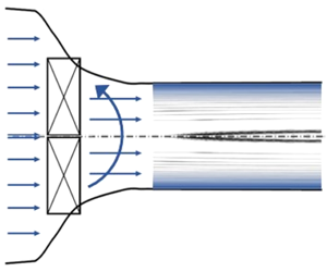
In this paper we focus on a model problem of a supersaturated vapour core in a humid air with swirl that enters a straight circular pipe of finite length. We assume that this inlet flow is generated from an upstream reservoir of humid air with non-saturated vapour phase, that is accelerated in a contracting circular nozzle, imparted rotation by a swirl generator (swirler), then achieves saturation of the vapour phase, crosses the state of equilibrium saturated vapour, further accelerated and achieves cooling conditions with no condensation and enters the pipe as a supersaturated swirling jet with thermal conditions for a possible onset of nucleation inside the pipe (see figure 1). The process of flow acceleration and cooling in the nozzle upstream of the pipe is complicated to simulate and is not modelled in this paper. Instead, it is replaced by flow and thermal conditions at the pipe inlet that may model it. The experiments of Panda & McLaughlin (Reference Panda and McLaughlin1994), Billant, Chomaz & Huerre (Reference Billant, Chomaz and Huerre1998), Leclaire & Jacquin (Reference Leclaire and Jacquin2012) and Oberleithner, Paschereit & Wygnanski (Reference Oberleithner, Paschereit and Wygnanski2014) used a contracting chamber apparatus and generated dry air swirling jets at the outlet of the chamber (inlet to a pipe test section). The Rusak et al. (Reference Rusak, Zhang, Lee and Wang2017) and Vanierschot (Reference Vanierschot2017) numerical studies also found that a contraction of swirling flows leads to a non-uniform acceleration of the axial velocity.
A passive, parallel (columnar) flow state is also assumed at the pipe exit. Extending the computational tools developed in Rusak et al. (Reference Rusak, Choi, Bourquard and Wang2015) for compressible, perfect-gas swirling flows in a circular contracting nozzle, such an apparatus ahead of the pipe can be carefully designed, built and used for experimental studies. Their approach relates a given upstream state with swirl, at the exit of a reservoir, and the resulting downstream state at the pipe inlet. A required state at the pipe inlet can be used to design the conditions at the reservoir exit.

Figure 1. Flow apparatus of swirling humid air with condensation.
We study the interaction between the compressible flow large-scale dynamics and the nanoscale condensation processes in the pipe to determine under the prescribed boundary conditions the flow structure and dynamics and the condensation process and zone. To the best of our knowledge, there are no existing experimental or numerical studies of this complicated flow problem. Also, there is no theoretical model that investigates the dynamics of compressible vortex flows of moist air in a pipe including condensation phenomena. A theoretical asymptotic analysis that simplifies the flow and condensation equations, specifically at near-critical swirl ratios around  $\unicode[STIX]{x1D714}_{1}$, may shed light for the first time on the complex phenomena in such flows.
The analysis uses simplifications, specifically about the condensation process. We note that similar simplifications were also used in numerical simulations of compressible flows of humid air around airfoils where they show agreement with experimental data, see for example Schnerr & Dohrmann (Reference Schnerr and Dohrmann1990, Reference Schnerr and Dohrmann1994).
A new small-disturbance model for the compressible swirling flow dynamics in the pipe with non-equilibrium and homogeneous condensation is developed. The mathematical model of the problem including the flow equations, condensation equations and assumed boundary conditions is described in § 2. The asymptotic analysis in § 3 explores the nonlinear interactions between the near-critical swirl ratio and the small amount of water vapour in the air. The critical state is defined in § 4. A model equation coupled with a set of four ordinary differential equations for the condensate (or sublimate) mass fraction buildup are derived in § 5. The theory developed in this paper can address any inlet flow profile including swirling jets found in the experimental studies. The computed examples in § 6 focus on an inlet flow described by the Lamb–Oseen vortex. Previous studies (Rusak, Whiting & Wang Reference Rusak, Whiting and Wang1998) show that the axisymmetric dynamics of swirling jets in a straight pipe and at very high Reynolds numbers is conceptually the same as that of the Lamb–Oseen vortex, i.e. the dynamics of a humid air Lamb–Oseen vortex represents all the important aspects of swirling jets and the difference is only in the numerical values of the critical swirls at  $\unicode[STIX]{x1D714}_{0}$ and
  $\unicode[STIX]{x1D714}_{1}$. These are important for a specific design of an experimental apparatus but not for the fundamental mechanism that governs the interaction between swirl and condensation. The model is used in § 6 to study effects of humidity level and energy supply from condensation on the dynamics of swirling jets in pipes as well as the effect of flow swirl on condensation processes in swirling jets. Conclusions and discussion of results are given in § 7. Appendix A provides empirical models for properties of water–ice and water–liquid. Appendix B gives details of derivations. Appendix C adds physical insight into vortex flows with condensation processes. Appendices A, B and C appear in the supplementary material, available at https://doi.org/10.1017/jfm.2019.1003.
2 Mathematical model
For many practical applications, atmospheric moist air can be modelled as a mixture of uniform, clean, dry air, water vapour and, when it exists, water condensate. Also, it is assumed that there is no chemical interaction between air and water and that molecules of air and water do not diffuse between flow particles. In the following, the subscripts  $a,v$ and
  $l$ denote properties of the dry air, water vapour and water condensate in the mixture, respectively, and a bar over a quantity indicates that it is dimensional. Let
  $\bar{\unicode[STIX]{x1D70C}}_{a}$,
  $\bar{\unicode[STIX]{x1D70C}}_{v}$ and
  $\bar{\unicode[STIX]{x1D70C}}_{l}$ be the partial densities of the air, water vapour and water condensate in a fluid element of the moist air, respectively (i.e. the mass of each constituent in a fluid element per its volume). Then, the density of a fluid element is
  $\bar{\unicode[STIX]{x1D70C}}=\bar{\unicode[STIX]{x1D70C}}_{a}+\bar{\unicode[STIX]{x1D70C}}_{v}+\bar{\unicode[STIX]{x1D70C}}_{l}$. In addition, we introduce the local initial specific humidity
  $\hat{\unicode[STIX]{x1D714}}=(\bar{\unicode[STIX]{x1D70C}}_{v}+\bar{\unicode[STIX]{x1D70C}}_{l})/\bar{\unicode[STIX]{x1D70C}}$ and the local condensate mass fraction
  $g=\bar{\unicode[STIX]{x1D70C}}_{l}/\bar{\unicode[STIX]{x1D70C}}$, such that
  $0\leqslant g\leqslant \hat{\unicode[STIX]{x1D714}}$. Then,
  $\bar{\unicode[STIX]{x1D70C}}_{v}=(\hat{\unicode[STIX]{x1D714}}-g)\bar{\unicode[STIX]{x1D70C}}$ and
  $\bar{\unicode[STIX]{x1D70C}}_{l}=g\bar{\unicode[STIX]{x1D70C}}$. The mixture also satisfies Dalton’s law of partial pressures, i.e. the absolute pressure
  $\bar{P}$ of an element is the sum of the partial pressures of the dry air and the water vapour,
  $\bar{P}=\bar{P}_{a}+\bar{P}_{v}$. The absolute temperature of an element is
  $\bar{T}$. Furthermore, assuming that the dry air and the water vapour each behave as thermally perfect gases, i.e.
  $\bar{P}_{a}=\bar{\unicode[STIX]{x1D70C}}_{a}(\bar{R}/\unicode[STIX]{x1D707}_{a})\bar{T}$ and
  $\bar{P}_{v}=\bar{\unicode[STIX]{x1D70C}}_{v}(\bar{R}/\unicode[STIX]{x1D707}_{v})\bar{T}$, we find that the mixture also behaves as a thermally perfect gas described the equation of state,
 $$\begin{eqnarray}\displaystyle \bar{P}=\bar{\unicode[STIX]{x1D70C}}\frac{\bar{R}}{\unicode[STIX]{x1D707}}\bar{T}. & & \displaystyle\end{eqnarray}$$
 Here  $\bar{R}$ is the universal gas constant,
  $\bar{R}=8.314~\text{J}~\text{mol}^{-1}~\text{K}^{-1}$ and
  $\unicode[STIX]{x1D707}$ is the local apparent molecular weight of the gas components of moist air and depends on the local initial specific humidity,
  $1/\unicode[STIX]{x1D707}=(1-\hat{\unicode[STIX]{x1D714}})/\unicode[STIX]{x1D707}_{a}+(\hat{\unicode[STIX]{x1D714}}-g)/\unicode[STIX]{x1D707}_{v}$, where
  $\unicode[STIX]{x1D707}_{a}$ and
  $\unicode[STIX]{x1D707}_{v}$ are the molecular weights of air and water, respectively. In addition, from (2.1) and the definitions of
  $\bar{\unicode[STIX]{x1D70C}}_{v}$ and
  $\unicode[STIX]{x1D707}$ we find that
 $$\begin{eqnarray}\displaystyle \bar{P}_{v}=\bar{P}\frac{(\hat{\unicode[STIX]{x1D714}}-g)}{(1-\hat{\unicode[STIX]{x1D714}})\displaystyle \frac{\unicode[STIX]{x1D707}_{v}}{\unicode[STIX]{x1D707}_{a}}+(\hat{\unicode[STIX]{x1D714}}-g)}. & & \displaystyle\end{eqnarray}$$
2.1 Flow equations
An unsteady, inviscid, compressible, axisymmetric, swirling flow of moist air is considered within a finite-length pipe of radius  $\bar{r}_{t}$. The centreline of the pipe is the
  $\bar{x}$-axis such that
  $\bar{x}$ measures axial distance from the pipe inlet and
  $0\leqslant \bar{x}\leqslant x_{0}\bar{r}_{t}$. Here
  $x_{0}$ is pipe non-dimensional length. A cylindrical coordinate system is used where the radial distance from the centreline is
  $\bar{r}$ and
  $0\leqslant \bar{r}\leqslant \bar{r}_{t}$. For all time
  $\bar{t}>0$, the moist air dynamics is described by the unsteady and axisymmetric equation of conservation of water mass and by the unsteady, inviscid and axisymmetric continuity, momentum and energy equations of the flow in the domain
  $0\leqslant \bar{x}\leqslant x_{0}\bar{r}_{t},0\leqslant \bar{r}\leqslant \bar{r}_{t}$,
 $$\begin{eqnarray}\displaystyle & \displaystyle \hat{\unicode[STIX]{x1D714}}_{\bar{t}}+\bar{u}\hat{\unicode[STIX]{x1D714}}_{\bar{r}}+\bar{w}\hat{\unicode[STIX]{x1D714}}_{\bar{x}}=0, & \displaystyle\end{eqnarray}$$
 $$\begin{eqnarray}\displaystyle & \displaystyle \bar{\unicode[STIX]{x1D70C}}_{\bar{t}}+(\bar{\unicode[STIX]{x1D70C}}\bar{u})_{\bar{r}}+\frac{\bar{\unicode[STIX]{x1D70C}}\bar{u}}{\bar{r}}+(\bar{\unicode[STIX]{x1D70C}}\bar{w})_{\bar{x}}=0, & \displaystyle\end{eqnarray}$$
 $$\begin{eqnarray}\displaystyle & \displaystyle \bar{\unicode[STIX]{x1D70C}}\left(\bar{u}_{\bar{t}}+\bar{u}\bar{u}_{\bar{r}}+\bar{w}\bar{u}_{\bar{x}}-\frac{\bar{v}^{2}}{\bar{r}}\right)=-\bar{P}_{\bar{r}}, & \displaystyle\end{eqnarray}$$
 $$\begin{eqnarray}\displaystyle & \displaystyle \bar{\unicode[STIX]{x1D70C}}(\bar{w}_{\bar{t}}+\bar{u}\bar{w}_{\bar{r}}+\bar{w}\bar{w}_{\bar{x}})=-\bar{P}_{\bar{x}}, & \displaystyle\end{eqnarray}$$
 $$\begin{eqnarray}\displaystyle & \displaystyle \bar{v}_{\bar{t}}+\bar{u}\bar{v}_{\bar{r}}+\bar{w}\bar{v}_{\bar{x}}+\frac{\bar{u}\bar{v}}{\bar{r}}=0, & \displaystyle\end{eqnarray}$$
 $$\begin{eqnarray}\displaystyle & \displaystyle \bar{\unicode[STIX]{x1D70C}}(\bar{h}_{\bar{t}}+\bar{u}\bar{h}_{\bar{r}}+\bar{w}\bar{h}_{\bar{x}})-(\bar{P}_{\bar{t}}+\bar{u}\bar{P}_{\bar{r}}+\bar{w}\bar{P}_{\bar{x}})=0. & \displaystyle\end{eqnarray}$$
 Here,  $\bar{u}$,
  $\bar{v}$ and
  $\bar{w}$ are the radial, circumferential and axial velocity components, respectively,
  $\bar{\unicode[STIX]{x1D70C}}$ is density and
  $\bar{P}$ is pressure. Also,
  $\bar{h}$ is the specific enthalpy of the moist air and can be rewritten in terms of the contributions from each of its constituents
 $$\begin{eqnarray}\displaystyle \bar{h}=(\bar{\unicode[STIX]{x1D70C}}_{a}\bar{h}_{a}+\bar{\unicode[STIX]{x1D70C}}_{v}\bar{h}_{v}+\bar{\unicode[STIX]{x1D70C}}_{l}\bar{h}_{l})/\bar{\unicode[STIX]{x1D70C}}=(1-\hat{\unicode[STIX]{x1D714}})\bar{C}_{pa}\bar{T}+\hat{\unicode[STIX]{x1D714}}\bar{C}_{pv}\bar{T}-g\bar{h}_{fg}(\bar{T}). & & \displaystyle\end{eqnarray}$$
 Here,  $\bar{T}$ is temperature. It is assumed that the air, water vapour and condensate specific enthalpies are given by
  $\bar{h}_{a}\sim \bar{C}_{pa}\bar{T},\bar{h}_{v}\sim \bar{h}_{g}(\bar{T})=\bar{C}_{pv}\bar{T}$ and
  $\bar{h}_{l}\sim \bar{h}_{f}(\bar{T})=\bar{h}_{g}(\bar{T})-\bar{h}_{fg}(\bar{T})$, respectively. Also,
  $\bar{C}_{pa}$ and
  $\bar{C}_{pv}$ are the air and water vapour specific heats for constant pressure processes, and are assumed constant,
  $\bar{C}_{pa}=\unicode[STIX]{x1D6FE}_{a}\bar{R}/[\unicode[STIX]{x1D707}_{a}(\unicode[STIX]{x1D6FE}_{a}-1)]$ and
  $\bar{C}_{pv}=\unicode[STIX]{x1D6FE}_{v}\bar{R}/[\unicode[STIX]{x1D707}_{v}(\unicode[STIX]{x1D6FE}_{v}-1)]$, where
  $\unicode[STIX]{x1D6FE}_{a}$ and
  $\unicode[STIX]{x1D6FE}_{v}$ are the ratio of specific heats of dry air and water vapour. The specific enthalpies of saturated water vapour and liquid,
  $\bar{h}_{g}$ and
  $\bar{h}_{f}$, and the latent heat resulting from the condensation from water vapour into liquid,
  $\bar{h}_{fg}$, are taken to be functions of temperature
  $\bar{T}$ only. Equations (2.8) and (2.9) account for the heat addition to the flow as a result of a condensation process. Notice that the heat source term vanishes in flow regions with no condensation (
 $g=0$). In regions where condensation occurs, we need to determine the condensate mass fraction,
  $g$.
$g$.
2.1.1 Condensation model equations
We assume that the classical nucleation theory of Hill (Reference Hill1966) for a non-equilibrium and homogeneous condensation process (with no molecular diffusion) describes the generation of condensate mass fraction,  $g$. The condensate rate equation can be generalized for an axisymmetric flow and is given in the domain
  $0\leqslant \bar{x}\leqslant x_{0}\bar{r}_{t},0\leqslant \bar{r}\leqslant \bar{r}_{t}$ by
 $$\begin{eqnarray}\displaystyle & \displaystyle (\bar{\unicode[STIX]{x1D70C}}\bar{r}g)_{\bar{t}}+(\bar{\unicode[STIX]{x1D70C}}\bar{w}\bar{r}g)_{\bar{x}}+(\bar{\unicode[STIX]{x1D70C}}\bar{u}\bar{r}g)_{\bar{r}}=4\unicode[STIX]{x03C0}\hat{\unicode[STIX]{x1D70C}}_{l}\left(\frac{1}{3}\bar{J}\bar{r}_{d}^{3}\bar{r}+\bar{\unicode[STIX]{x1D70C}}\bar{Q}_{1}\frac{\text{d}\bar{r}_{d}}{\text{d}\bar{t}}\bar{r}\right), & \displaystyle\end{eqnarray}$$
 $$\begin{eqnarray}\displaystyle & \displaystyle (\bar{\unicode[STIX]{x1D70C}}\bar{r}\bar{Q}_{1})_{\bar{t}}+(\bar{\unicode[STIX]{x1D70C}}\bar{w}\bar{r}\bar{Q}_{1})_{\bar{x}}+(\bar{\unicode[STIX]{x1D70C}}\bar{u}\bar{r}\bar{Q}_{1})_{\bar{r}}=\bar{J}\bar{r}_{d}^{2}\bar{r}+2\bar{\unicode[STIX]{x1D70C}}\bar{Q}_{2}\frac{\text{d}\bar{r}_{d}}{\text{d}\bar{t}}\bar{r}, & \displaystyle\end{eqnarray}$$
 $$\begin{eqnarray}\displaystyle & \displaystyle (\bar{\unicode[STIX]{x1D70C}}\bar{r}\bar{Q}_{2})_{\bar{t}}+(\bar{\unicode[STIX]{x1D70C}}\bar{w}\bar{r}\bar{Q}_{2})_{\bar{x}}+(\bar{\unicode[STIX]{x1D70C}}\bar{u}\bar{r}\bar{Q}_{2})_{\bar{r}}=\bar{J}\bar{r}_{d}\bar{r}+\bar{\unicode[STIX]{x1D70C}}\bar{Q}_{3}\frac{\text{d}\bar{r}_{d}}{\text{d}\bar{t}}\bar{r}, & \displaystyle\end{eqnarray}$$
 $$\begin{eqnarray}\displaystyle & \displaystyle (\bar{\unicode[STIX]{x1D70C}}\bar{r}\bar{Q}_{3})_{\bar{t}}+(\bar{\unicode[STIX]{x1D70C}}\bar{w}\bar{r}\bar{Q}_{3})_{\bar{x}}+(\bar{\unicode[STIX]{x1D70C}}\bar{u}\bar{r}\bar{Q}_{3})_{\bar{r}}=\bar{J}\bar{r}. & \displaystyle\end{eqnarray}$$
 Here, the nucleation variables are:  $\bar{Q}_{1}$ the sum of droplet surface areas over
  $4\unicode[STIX]{x03C0}$ per unit mass of fluid element,
  $\bar{Q}_{2}$ the sum of droplet radii per unit mass of fluid element,
  $\bar{Q}_{3}$ the sum of droplets per unit mass of fluid element. The initial radius of a nucleus of condensation is
  $\bar{r}_{d}$, the droplet growth rate is
  $\text{d}\bar{r}_{d}/\text{d}\bar{t}$ and the rate of nucleation is
  $\bar{J}$. Also,
  $\hat{\unicode[STIX]{x1D70C}}_{l}$ is the density of liquid water.
Following Hill (Reference Hill1966), we assume that  $\bar{r}_{d}=1.3\bar{r}^{\ast }$ where
  $\bar{r}^{\ast }$ is the critical radius of a droplet. We account for some possible delay in droplet growth from critical size. Using the balance of stresses on a droplet surface at critical size and the Thomson–Gibbs equation, we have
 $$\begin{eqnarray}\displaystyle \bar{r}^{\ast }=\frac{2\bar{\unicode[STIX]{x1D70E}}_{\infty }(\bar{T})}{\hat{\unicode[STIX]{x1D70C}}_{l}(\bar{R}/\unicode[STIX]{x1D707}_{v})\bar{T}\ln (S)}. & & \displaystyle\end{eqnarray}$$
 Here,  $\bar{\unicode[STIX]{x1D70E}}_{\infty }(\bar{T})$ is the surface tension of a plane surface with an infinite curvature and
  $S$ is the supersaturation ratio given in terms of the saturation pressure
  $\bar{P}_{g}(\bar{T})$
 $$\begin{eqnarray}\displaystyle S=\frac{\bar{P}_{v}}{\bar{P}_{g}(\bar{T})}. & & \displaystyle\end{eqnarray}$$
When the temperature of the water vapour and of the liquid droplet in a particle are the same, the droplet growth rate is given by the Hertz–Knudsen model,
 $$\begin{eqnarray}\displaystyle \frac{\text{d}\bar{r}_{d}}{\text{d}\bar{t}}=\frac{\unicode[STIX]{x1D6FC}(\bar{T})}{\hat{\unicode[STIX]{x1D70C}}_{l}}\frac{\bar{P}_{v}-\bar{P}_{g}(\bar{T})}{\sqrt{2\unicode[STIX]{x03C0}(\bar{R}/\unicode[STIX]{x1D707}_{v})\bar{T}}}, & & \displaystyle\end{eqnarray}$$
 where  $\unicode[STIX]{x1D6FC}(\bar{T})$ is a non-dimensional condensation coefficient which represents the proportion of molecules impinging on a droplet surface that actually stick to it.
This set of molecular scalings implies an assumption of no slip between condensate droplets and the surrounding vapour–carrier gas phase. We find that in all the flow cases studied in this paper, the critical radii for nucleation are in the range of 0.6 nm. Also, in all the cases presented we find that the maximum radius of droplets (as estimated from maximum value of  $\bar{Q}_{2}/\bar{Q}_{3}$) in the region of condensation is less than
  $0.1~\unicode[STIX]{x03BC}\text{m}$, which is much smaller than the size of a typical humid air fluid element. Then, the maximum droplet size remains within the order of molecular scaling and therefore no slip between droplets and the gas–vapour phases may be justified, even in presence of axial and centripetal accelerations.
The rate of nucleation is the number of droplets per unit time and volume of a fluid element and is given by
 $$\begin{eqnarray}\displaystyle \bar{J}=\sqrt{\frac{2\bar{\unicode[STIX]{x1D70E}}_{\infty }(\bar{T})}{\unicode[STIX]{x03C0}}}m^{-3/2}\frac{\bar{\unicode[STIX]{x1D70C}}_{v}^{2}}{\hat{\unicode[STIX]{x1D70C}}_{l}}\exp \left(\frac{-\bar{W}^{\ast }}{k\bar{T}}\right). & & \displaystyle\end{eqnarray}$$
 Here,  $m$ is the mass of a molecule of water,
  $m=3\times 10^{-26}~\text{kg}$, and
  $k$ is Boltzmann’s constant,
  $k=1.3806503\times 10^{-23}~\text{m}^{2}~\text{kg}~\text{s}^{-2}~\text{K}^{-1}$. The critical work
  $\bar{W}^{\ast }$ is computed from the difference between the work done against the surface tension to increase the surface area of a spherical droplet and the work expended by the pressure difference inside and outside the droplet to increase the volume of the droplet. It can be shown that
 $$\begin{eqnarray}\displaystyle \bar{W}^{\ast }=\frac{16\unicode[STIX]{x03C0}}{3}\left(\frac{m}{\hat{\unicode[STIX]{x1D70C}}_{l}\ln (S)k\bar{T}}\right)^{2}\bar{\unicode[STIX]{x1D70E}}_{\infty }^{3}(\bar{T}). & & \displaystyle\end{eqnarray}$$
 Empirical formulae from Schnerr & Dohrmann (Reference Schnerr and Dohrmann1990) for  $\bar{P}_{g}(\bar{T})$,
  $\hat{\unicode[STIX]{x1D70C}}_{l}(\bar{T}),\bar{\unicode[STIX]{x1D70E}}_{\infty }(\bar{T})$ and
  $\unicode[STIX]{x1D6FC}(\bar{T})$ for water–liquid and for water–ice properties are given in supplementary appendix A.
2.2 Boundary conditions
Equations (2.10)–(2.13) describe the generation of the condensate within the flow. Together with (2.1)–(2.9), we have a system of equations describing the evolution of an inviscid swirling flow of moist air with non-equilibrium and homogeneous condensation. We look for a solution of the flow in a circular, straight, finite-length pipe under the following boundary conditions.
2.2.1 Inlet conditions
At the pipe inlet  $\bar{x}=0$, a moist air vortex state is given for all times by the profiles of the initial specific humidity, axial and circumferential velocities, azimuthal vorticity and temperature,
 $$\begin{eqnarray}\displaystyle \left.\begin{array}{@{}c@{}}\displaystyle \hat{\unicode[STIX]{x1D714}}(\bar{t},0,\bar{r})=\tilde{\unicode[STIX]{x1D714}}_{0}\hat{\unicode[STIX]{x1D714}}_{0}(\bar{r}/\bar{r}_{t}),\\ \displaystyle \bar{w}(\bar{t},0,\bar{r})=\bar{U}_{0}w_{0}(\bar{r}/\bar{r}_{t}),\\ \displaystyle \bar{v}(\bar{t},0,\bar{r})=\unicode[STIX]{x1D714}\bar{U}_{0}v_{0}(\bar{r}/\bar{r}_{t}),\\ \displaystyle \bar{\unicode[STIX]{x1D702}}(\bar{t},0,\bar{r})=\frac{\bar{U}_{0}}{\bar{r}_{t}}\unicode[STIX]{x1D702}_{0}(\bar{r}/\bar{r}_{t}),\\ \displaystyle \bar{T}(\bar{t},0,\bar{r})=\bar{T}_{0}T_{0}(\bar{r}/\bar{r}_{t}),\end{array}\right\} & & \displaystyle\end{eqnarray}$$
 for  $0\leqslant \bar{r}\leqslant \bar{r}_{t}$. All inlet profiles in (2.19) are given by a reference scaling value and a shape function. Here,
  $\tilde{\unicode[STIX]{x1D714}}_{0}$ is the inlet centreline specific humidity (
 $0<\tilde{\unicode[STIX]{x1D714}}_{0}\ll 1$),
  $\hat{\unicode[STIX]{x1D714}}_{0}(\bar{r}/\bar{r}_{t})$ is a shape function that has a value of unity at the centreline. Also,
  $\bar{U}_{0}$ is the axial centreline velocity at the pipe inlet,
  $\unicode[STIX]{x1D714}$ is the incoming swirl ratio,
  $\bar{\unicode[STIX]{x1D702}}=\bar{u}_{\bar{x}}-\bar{w}_{\bar{r}}$ is the azimuthal vorticity and
  $\bar{T}_{0}$ is the temperature at the inlet centreline. Further symmetry conditions are imposed at the inlet centreline, namely
  $\hat{\unicode[STIX]{x1D714}}_{0r}(0)=0,w_{0\bar{r}}(0)=0$,
  $v_{0}(0)=0$ and
  $T_{0\bar{r}}(0)=0$. We also assume that the inlet wall pressure is fixed,
 $$\begin{eqnarray}\displaystyle \bar{P}(\bar{t},0,\bar{r}_{t})=\bar{P}_{0}. & & \displaystyle\end{eqnarray}$$
The inlet conditions (2.19) represent a state of a swirling flow of a supersaturated humid air downstream of a reservoir of non-saturated vapour phase in a humid air that also includes a vortex generator ahead of the pipe at a steady and continuous operation (see again figure 1). Thereby, these conditions replace the necessary complicated simulation of the development and cooling of the humid air swirling flow in the contracting section ahead of the pipe to the pipe inlet. It is also postulated that there is no condensation in the contracting section. The vortex generation and flow contraction processes to a supersaturated inlet state are not of interest in this study; rather, the focus is on flow and condensation structure and flow dynamics in the pipe as a result of these assumed inlet conditions.
Following Wang & Rusak (Reference Wang and Rusak1996, Reference Wang and Rusak1997), we specifically focus on the essential case where
 $$\begin{eqnarray}\displaystyle \bar{\unicode[STIX]{x1D702}}_{0}=-\bar{w}_{0\bar{r}}\quad \text{or}\quad \bar{u}_{\bar{x}}(\bar{t},0,\bar{r})=0, & & \displaystyle\end{eqnarray}$$
 for  $0\leqslant \bar{r}\leqslant \bar{r}_{t}$. The condition (2.21) allows the inlet state a degree of freedom to develop a radial velocity, to replicate the upstream effect of disturbances in the flow that have the ability to create such an influence.
In addition, at the inlet we assume that the incoming flow consists for all times of no condensate and zero values for the nucleation variables i.e.
 $$\begin{eqnarray}\displaystyle \left.\begin{array}{@{}c@{}}g(\bar{t},0,\bar{r})=0,\quad \bar{Q}_{1}(\bar{t},0,\bar{r})=0,\\ \bar{Q}_{2}(\bar{t},0,\bar{r})=0,\quad \bar{Q}_{3}(\bar{t},0,\bar{r})=0.\end{array}\right\} & & \displaystyle\end{eqnarray}$$
 The inlet flow is characterized by a Mach number,  $Ma_{0}=\bar{U}_{0}/a_{0}$ where
  $a_{0}$ is the local isentropic speed of sound of the moist air at the inlet centreline,
  $a_{0}=\sqrt{\unicode[STIX]{x1D6FE}_{0}\bar{R}\bar{T}_{0}/\unicode[STIX]{x1D707}_{a}}$. Here
  $\unicode[STIX]{x1D6FE}_{0}$ is the inlet centreline ratio of specific heats and
  $\unicode[STIX]{x1D707}_{0}$ is the local inlet centreline apparent molecular weight,
  $\unicode[STIX]{x1D6FE}_{0}=[(1-\tilde{\unicode[STIX]{x1D714}}_{0})\bar{C}_{pa}+\tilde{\unicode[STIX]{x1D714}}_{0}\bar{C}_{pv}]/[(1-\tilde{\unicode[STIX]{x1D714}}_{0})\bar{C}_{va}+\tilde{\unicode[STIX]{x1D714}}_{0}\bar{C}_{vv}]$ and
  $1/\unicode[STIX]{x1D707}_{0}=((1-\tilde{\unicode[STIX]{x1D714}}_{0})/\unicode[STIX]{x1D707}_{a})+\tilde{\unicode[STIX]{x1D714}}_{0}/\unicode[STIX]{x1D707}_{v}$.
2.2.2 Outlet conditions
For a long, open pipe,  $x_{0}\gg 1$, we assume at the outlet a fully developed state with zero radial velocity and non-reflective Neumann conditions on all the other variables, i.e. at
  $\bar{x}=x_{0}\bar{r}_{t}$,
 $$\begin{eqnarray}\displaystyle \left.\begin{array}{@{}c@{}}\bar{u}(\bar{t},x_{0}\bar{r}_{t},\bar{r})=0,\quad \bar{w}_{\bar{t}}(\bar{t},x_{0}\bar{r}_{t},\bar{r})+\bar{w}\bar{w}_{\bar{x}}(\bar{t},x_{0}\bar{r}_{t},\bar{r})=0,\\ \bar{v}_{\bar{t}}(\bar{t},x_{0}\bar{r}_{t},\bar{r})+\bar{w}\bar{v}_{\bar{x}}(\bar{t},x_{0}\bar{r}_{t},\bar{r})=0,\\ \bar{P}_{\bar{t}}(\bar{t},x_{0}\bar{r}_{t},\bar{r})+\bar{w}\bar{P}_{\bar{x}}(\bar{t},x_{0}\bar{r}_{t},\bar{r})=0,\quad \bar{T}_{\bar{t}}(\bar{t},x_{0}\bar{r}_{t},\bar{r})+\bar{w}\bar{T}_{\bar{x}}(\bar{t},x_{0}\bar{r}_{t},\bar{r})=0.\end{array}\right\} & & \displaystyle\end{eqnarray}$$
2.2.3 Centreline and wall conditions
The flow is subjected at all times to symmetry conditions along the pipe centreline  $\bar{r}=0$, i.e.
 $$\begin{eqnarray}\displaystyle \left.\begin{array}{@{}c@{}}\hat{\unicode[STIX]{x1D714}}_{\bar{r}}(\bar{t},\bar{x},0)=0,\quad \bar{u}(\bar{t},\bar{x},0)=0,\\ \bar{v}(\bar{t},\bar{x},0)=0,\quad \bar{w}_{\bar{r}}(\bar{t},\bar{x},0)=0,\\ \bar{T}_{\bar{r}}(\bar{t},\bar{x},0)=0,\quad \bar{P}_{\bar{r}}(\bar{t},\bar{x},0)=0,\\ g_{\bar{r}}(\bar{t},\bar{x},0)=\bar{Q}_{1\bar{r}}(\bar{t},\bar{x},0)=\bar{Q}_{2\bar{r}}(\bar{t},\bar{x},0)=\bar{Q}_{3\bar{r}}(\bar{t},\bar{x},0)=0,\end{array}\right\} & & \displaystyle\end{eqnarray}$$
 for  $0\leqslant \bar{x}\leqslant x_{0}\bar{r}_{t}$. Furthermore, no flow penetration along the pipe wall requires that the radial velocity component vanishes at all times at
  $\bar{r}=\bar{r}_{t}$ for
  $0\leqslant \bar{x}\leqslant x_{0}\bar{r}_{t}$.
 $$\begin{eqnarray}\displaystyle \bar{u}(\bar{t},\bar{x},\bar{r}_{t})=0. & & \displaystyle\end{eqnarray}$$
 The flow equations (2.1)–(2.9) together with nucleation equations (2.10)–(2.13) and the boundary conditions (2.19)–(2.25) describe a well-defined problem of the compressible dynamics and concurrent nucleation processes of an inviscid swirling flow of moist air in a straight, circular, finite-length pipe. There are seven flow equations and four nucleation equations supported by eleven inlet and outlet conditions (seven conditions on the flow variables and four inlet conditions on the nucleation variables) and by eleven centreline-and-wall conditions (seven conditions on the flow variables and four centreline conditions on the nucleation variables). Given initial conditions, for example an  $x$-independent columnar state where for all
  $x$ the flow and nucleation variables are equal to the inlet profiles, the moist air flow evolution can be integrated in time. The problem is dominated by the size of pipe radius
  $\bar{r}_{t}$, the inlet speed
  $\bar{U}_{0}$, the inlet swirl ratio
  $\unicode[STIX]{x1D714}$, the inlet centreline temperature and pressure
  $\bar{T}_{0}$ and
  $\bar{P}_{0}$, and the inlet centreline specific humidity,
  $\tilde{\unicode[STIX]{x1D714}}_{0}$. We specifically look to establish steady-state solutions of the problem and determine the stability of those states.
In this paper, we study applications where the amount of water in the air is small,  $0\leqslant \tilde{\unicode[STIX]{x1D714}}_{0}\ll 1$. Moreover, our interest is in the flow behaviour when the swirl ratio is near critical
  $|\unicode[STIX]{x0394}\unicode[STIX]{x1D714}|/\unicode[STIX]{x1D714}_{1}\ll 1$ where
  $\unicode[STIX]{x0394}\unicode[STIX]{x1D714}=\unicode[STIX]{x1D714}-\unicode[STIX]{x1D714}_{1}$. Then the problem is amenable to a small disturbance analysis in the limit when
  $\unicode[STIX]{x1D714}\rightarrow \unicode[STIX]{x1D714}_{1}$ and
  $\tilde{\unicode[STIX]{x1D714}}_{0}\rightarrow 0$ with fixed values of
  $Ma_{0}$,
  $\bar{T}_{0}$ and
  $\bar{P}_{0}$. Note that in the limit case of a columnar (
 $x$-independent) swirling flow of dry air
  $\tilde{\unicode[STIX]{x1D714}}_{0}=0$, the state is a base solution of the problem for every
  $\mathit{Ma}_{0}$,
  $\bar{T}_{0},\bar{P}_{0}$ and
  $\unicode[STIX]{x1D714}$, and for all
  $\bar{x}$ and
  $\bar{t}$. This branch of columnar states exhibits a transcritical bifurcation of additional non-columnar steady states at the critical swirl
  $\unicode[STIX]{x1D714}=\unicode[STIX]{x1D714}_{1}$ and the structure and stability of the bifurcating states were studied in Rusak et al. (Reference Rusak, Choi and Lee2007). Here we look at the nonlinear interaction between the condensation process and the swirling flow at near-critical situations and establish the modified bifurcation diagrams and stability characteristics due to non-equilibrium and homogeneous condensation.
3 Perturbation equations
In the following, we use the scalings  $t=\bar{t}\bar{U}_{0}|\unicode[STIX]{x0394}\unicode[STIX]{x1D714}|/\bar{r}_{t}$,
  $r=\bar{r}/\bar{r}_{t}$ and
  $x=\bar{x}/\bar{r}_{t}$.
3.1 Flow perturbation equations
In order to study the effect of humidity  $\hat{\unicode[STIX]{x1D714}}$ and condensate
  $g$ on near-critical swirling flows we consider the following asymptotic expansions:
 $$\begin{eqnarray}\displaystyle \hat{\unicode[STIX]{x1D714}}=\tilde{\unicode[STIX]{x1D714}}_{0}[\tilde{\unicode[STIX]{x1D714}}(t,x,r)+\cdots \,]\quad \text{and}\quad g=\tilde{\unicode[STIX]{x1D714}}_{0}[\tilde{g}(t,x,r)+\cdots \,], & & \displaystyle\end{eqnarray}$$
 $$\begin{eqnarray}\displaystyle & \displaystyle \bar{\unicode[STIX]{x1D70C}}=\bar{\unicode[STIX]{x1D70C}}_{0}[\unicode[STIX]{x1D70C}_{0}(r)+\unicode[STIX]{x1D6FE}_{0}\mathit{Ma}_{0}^{2}\unicode[STIX]{x1D716}_{1}(t)\unicode[STIX]{x1D70C}_{1}(x,r)+\unicode[STIX]{x1D6FE}_{0}\mathit{Ma}_{0}^{2}\unicode[STIX]{x1D716}_{2}(t)\unicode[STIX]{x1D70C}_{2}(x,r)+\cdots \,], & \displaystyle\end{eqnarray}$$
 $$\begin{eqnarray}\displaystyle & \displaystyle \bar{T}=\bar{T}_{0}[T_{0}(r)+\unicode[STIX]{x1D6FE}_{0}\mathit{Ma}_{0}^{2}\unicode[STIX]{x1D716}_{1}(t)T_{1}(x,r)+\unicode[STIX]{x1D6FE}_{0}\mathit{Ma}_{0}^{2}\unicode[STIX]{x1D716}_{2}(t)T_{2}(x,r)+\cdots \,], & \displaystyle\end{eqnarray}$$
 $$\begin{eqnarray}\displaystyle & \displaystyle \bar{P}=\bar{P}_{0}[P_{0}(r)+\unicode[STIX]{x1D6FE}_{0}\mathit{Ma}_{0}^{2}\unicode[STIX]{x1D716}_{1}(t)P_{1}(x,r)+\unicode[STIX]{x1D6FE}_{0}\mathit{Ma}_{0}^{2}\unicode[STIX]{x1D716}_{2}(t)P_{2}(x,r)+\cdots \,], & \displaystyle\end{eqnarray}$$
 $$\begin{eqnarray}\displaystyle & \displaystyle \bar{u}=\bar{U}_{0}[\unicode[STIX]{x1D716}_{1}(t)u_{1}(x,r)+\unicode[STIX]{x1D716}_{2}(t)u_{2}(x,r)+\cdots \,], & \displaystyle\end{eqnarray}$$
 $$\begin{eqnarray}\displaystyle & \displaystyle \bar{v}=\bar{U}_{0}[\unicode[STIX]{x1D714}v_{0}(r)+\unicode[STIX]{x1D716}_{1}(t)v_{1}(x,r)+\unicode[STIX]{x1D716}_{2}(t)v_{2}(x,r)+\cdots \,], & \displaystyle\end{eqnarray}$$
 $$\begin{eqnarray}\displaystyle & \displaystyle \bar{w}=\bar{U}_{0}[w_{0}(r)+\unicode[STIX]{x1D716}_{1}(t)w_{1}(x,r)+\unicode[STIX]{x1D716}_{2}(t)w_{2}(x,r)+\cdots \,], & \displaystyle\end{eqnarray}$$
 with  $\unicode[STIX]{x1D714}=\unicode[STIX]{x1D714}_{1}+\unicode[STIX]{x0394}\unicode[STIX]{x1D714}$. Here
  $\unicode[STIX]{x1D716}_{1}$ is the leading-order perturbation’s amplitude and
  $\unicode[STIX]{x1D716}_{2}$ is the second-order perturbation’s amplitude such that
  $|\unicode[STIX]{x1D716}_{2}|\ll |\unicode[STIX]{x1D716}_{1}|\ll 1$. In addition,
  $\unicode[STIX]{x1D70C}_{1}$,
  $T_{1}$,
  $P_{1}$,
  $u_{1}$,
  $v_{1}$ and
  $w_{1}$ are the leading-order perturbation’s shape functions and
  $\unicode[STIX]{x1D70C}_{2}$,
  $T_{2}$,
  $P_{2}$,
  $u_{2}$,
  $v_{2}$ and
  $w_{2}$ are the second-order perturbation’s shape functions. Furthermore, it is assumed that
  $\unicode[STIX]{x1D716}_{2}\sim \unicode[STIX]{x1D716}_{1}^{2}\sim \unicode[STIX]{x1D716}_{1t}|\unicode[STIX]{x0394}\unicode[STIX]{x1D714}|\sim \unicode[STIX]{x1D716}_{1}\unicode[STIX]{x0394}\unicode[STIX]{x1D714}\sim \tilde{\unicode[STIX]{x1D714}}_{0}$. Also, let
  $\bar{\unicode[STIX]{x1D70C}}_{0}=\bar{P}_{0}\unicode[STIX]{x1D707}_{a}/(\bar{R}\bar{T}_{0})$.
Substituting the expressions (3.1)–(3.7) into the equation of state for moist air (2.1), flow equations (2.3)–(2.8) and the extended definition of enthalpy (2.9), we first arrive at the following leading-order relations:
 $$\begin{eqnarray}\displaystyle & \displaystyle O(1):P_{0}=\unicode[STIX]{x1D70C}_{0}T_{0}, & \displaystyle\end{eqnarray}$$
 $$\begin{eqnarray}\displaystyle & \displaystyle O(1):P_{0r}=\frac{\unicode[STIX]{x1D6FE}_{0}\mathit{Ma}_{0}^{2}\unicode[STIX]{x1D70C}_{0}\unicode[STIX]{x1D714}^{2}v_{0}^{2}}{r}. & \displaystyle\end{eqnarray}$$
 The solution of (3.8) and (3.9) gives for all  $\mathit{Ma}_{0},\unicode[STIX]{x1D714}$ and
  $\tilde{\unicode[STIX]{x1D714}}_{0}$ the leading-order pressure in terms of the leading-order temperature and swirl profile.
 $$\begin{eqnarray}\displaystyle P_{0}(r)=\exp \left(\unicode[STIX]{x1D6FE}_{0}Ma_{0}^{2}\unicode[STIX]{x1D714}^{2}\int _{1}^{r}\frac{v_{0}^{2}(r^{\prime })}{r^{\prime }T_{0}(r^{\prime })}\,\text{d}r^{\prime }\right). & & \displaystyle\end{eqnarray}$$
 Note that  $P_{0}(r)$ is also a function of
  $\tilde{\unicode[STIX]{x1D714}}_{0}$ through its effect on
  $\unicode[STIX]{x1D6FE}_{0}$ and
  $\mathit{Ma}_{0}$.
The first- and second-order perturbation equations in domain  $0\leqslant x\leqslant x_{0},0\leqslant r\leqslant 1$ are as follows.
From conservation of water mass (2.3),  $\tilde{\unicode[STIX]{x1D714}}_{x}=0$ or
  $\tilde{\unicode[STIX]{x1D714}}=\hat{\unicode[STIX]{x1D714}}_{0}(r)$. Higher-order terms of
  $\tilde{\unicode[STIX]{x1D714}}$ can be computed but are not needed for further analysis.
From the equation of state (2.1),
 $$\begin{eqnarray}\displaystyle O(\unicode[STIX]{x1D716}_{1}):P_{1}=\unicode[STIX]{x1D70C}_{1}T_{0}+\unicode[STIX]{x1D70C}_{0}T_{1}, & & \displaystyle\end{eqnarray}$$
 $$\begin{eqnarray}\displaystyle & & \displaystyle O(\unicode[STIX]{x1D716}_{2},\unicode[STIX]{x1D716}_{1}^{2},\tilde{\unicode[STIX]{x1D714}}_{0}):\unicode[STIX]{x1D716}_{2}(P_{2}-\unicode[STIX]{x1D70C}_{2}T_{0}-\unicode[STIX]{x1D70C}_{0}T_{2})\nonumber\\ \displaystyle & & \displaystyle \quad =\frac{T_{0}\unicode[STIX]{x1D70C}_{0}}{\unicode[STIX]{x1D6FE}_{0}\mathit{Ma}_{0}^{2}}\tilde{\unicode[STIX]{x1D714}}_{0}((\hat{\unicode[STIX]{x1D714}}_{0}(r)-\tilde{g})\unicode[STIX]{x1D707}_{a}/\unicode[STIX]{x1D707}_{v}-\hat{\unicode[STIX]{x1D714}}_{0}(r))+\unicode[STIX]{x1D716}_{1}^{2}\unicode[STIX]{x1D6FE}_{0}\mathit{Ma}_{0}^{2}\unicode[STIX]{x1D70C}_{1}T_{1}.\end{eqnarray}$$
From the continuity equation (2.4),
 $$\begin{eqnarray}\displaystyle O(\unicode[STIX]{x1D716}_{1}):\frac{1}{r}(r\unicode[STIX]{x1D70C}_{0}u_{1})_{r}+(\unicode[STIX]{x1D70C}_{0}w_{1}+\unicode[STIX]{x1D6FE}_{0}\mathit{Ma}_{0}^{2}\unicode[STIX]{x1D70C}_{1}w_{0})_{x}=0, & & \displaystyle\end{eqnarray}$$
 $$\begin{eqnarray}\displaystyle & & \displaystyle O(\unicode[STIX]{x1D716}_{2},\unicode[STIX]{x1D716}_{1}^{2},\unicode[STIX]{x1D716}_{1t}|\unicode[STIX]{x0394}\unicode[STIX]{x1D714}|):\unicode[STIX]{x1D716}_{2}\left(\frac{1}{r}(r\unicode[STIX]{x1D70C}_{0}u_{2})+\unicode[STIX]{x1D70C}_{0}w_{2x}+\unicode[STIX]{x1D6FE}_{0}\mathit{Ma}_{0}^{2}w_{0}\unicode[STIX]{x1D70C}_{2x}\right)\nonumber\\ \displaystyle & & \displaystyle \quad =-\unicode[STIX]{x1D716}_{1t}|\unicode[STIX]{x0394}\unicode[STIX]{x1D714}|(\unicode[STIX]{x1D6FE}_{0}\mathit{Ma}_{0}^{2}\unicode[STIX]{x1D70C}_{1})-\unicode[STIX]{x1D716}_{1}^{2}\unicode[STIX]{x1D6FE}_{0}\mathit{Ma}_{0}^{2}\left(\frac{1}{r}(r\unicode[STIX]{x1D70C}_{1}u_{1})_{r}+(\unicode[STIX]{x1D70C}_{1}w_{1})_{x}\right).\end{eqnarray}$$
From the radial momentum equation (2.5),
 $$\begin{eqnarray}\displaystyle O(\unicode[STIX]{x1D716}_{1}):\unicode[STIX]{x1D70C}_{0}w_{0}u_{1x}-\frac{2}{r}\unicode[STIX]{x1D714}_{1}v_{0}\unicode[STIX]{x1D70C}_{0}v_{1}-\unicode[STIX]{x1D6FE}_{0}\mathit{Ma}_{0}^{2}\unicode[STIX]{x1D714}_{1}^{2}\frac{v_{0}^{2}}{r}\unicode[STIX]{x1D70C}_{1}=-P_{1r}, & & \displaystyle\end{eqnarray}$$
 $$\begin{eqnarray}\displaystyle & & \displaystyle O(\unicode[STIX]{x1D716}_{2},\unicode[STIX]{x1D716}_{1}^{2},\unicode[STIX]{x1D716}_{1t}|\unicode[STIX]{x0394}\unicode[STIX]{x1D714}|,\unicode[STIX]{x1D716}_{1}\unicode[STIX]{x0394}\unicode[STIX]{x1D714}):\unicode[STIX]{x1D716}_{2}\left(\unicode[STIX]{x1D70C}_{0}w_{0}u_{2x}-\frac{2}{r}\unicode[STIX]{x1D714}_{1}v_{0}\unicode[STIX]{x1D70C}_{0}v_{2}-\unicode[STIX]{x1D6FE}_{0}\mathit{Ma}_{0}^{2}\unicode[STIX]{x1D714}_{1}^{2}\frac{v_{0}^{2}}{r}\unicode[STIX]{x1D70C}_{2}+P_{2r}\right)\nonumber\\ \displaystyle & & \displaystyle \quad =-\unicode[STIX]{x1D716}_{1t}|\unicode[STIX]{x0394}\unicode[STIX]{x1D714}|(\unicode[STIX]{x1D70C}_{0}u_{1})-\unicode[STIX]{x1D716}_{1}^{2}\left[\unicode[STIX]{x1D70C}_{0}u_{1}u_{1r}+\unicode[STIX]{x1D70C}_{0}w_{1}u_{1x}-\unicode[STIX]{x1D70C}_{0}\frac{v_{1}^{2}}{r}\right.\nonumber\\ \displaystyle & & \displaystyle \qquad \quad +\left.\unicode[STIX]{x1D6FE}_{0}\mathit{Ma}_{0}^{2}(w_{0}\unicode[STIX]{x1D70C}_{1}u_{1x}-\frac{2}{r}\unicode[STIX]{x1D714}_{1}v_{0}v_{1}\unicode[STIX]{x1D70C}_{1})\right]\nonumber\\ \displaystyle & & \displaystyle \qquad \quad +\,2\unicode[STIX]{x1D716}_{1}\unicode[STIX]{x0394}\unicode[STIX]{x1D714}\left(\frac{1}{r}v_{0}\unicode[STIX]{x1D70C}_{0}v_{1}+\unicode[STIX]{x1D6FE}_{0}\mathit{Ma}_{0}^{2}\unicode[STIX]{x1D714}_{1}\frac{v_{0}^{2}}{r}\unicode[STIX]{x1D70C}_{1}\right).\end{eqnarray}$$
From the axial momentum equation (2.6),
 $$\begin{eqnarray}\displaystyle O(\unicode[STIX]{x1D716}_{1}):\unicode[STIX]{x1D70C}_{0}w_{0r}u_{1}+\unicode[STIX]{x1D70C}_{0}w_{0}w_{1x}=-P_{1x}, & & \displaystyle\end{eqnarray}$$
 $$\begin{eqnarray}\displaystyle & & \displaystyle O(\unicode[STIX]{x1D716}_{2},\unicode[STIX]{x1D716}_{1}^{2},\unicode[STIX]{x1D716}_{1t}|\unicode[STIX]{x0394}\unicode[STIX]{x1D714}|):\unicode[STIX]{x1D716}_{2}(\unicode[STIX]{x1D70C}_{0}w_{0r}u_{2}+\unicode[STIX]{x1D70C}_{0}w_{0}w_{2x}+P_{2x})=-\unicode[STIX]{x1D716}_{1t}|\unicode[STIX]{x0394}\unicode[STIX]{x1D714}|(\unicode[STIX]{x1D70C}_{0}w_{1})\nonumber\\ \displaystyle & & \displaystyle \quad -\,\unicode[STIX]{x1D716}_{1}^{2}[\unicode[STIX]{x1D70C}_{0}u_{1}w_{1r}+\unicode[STIX]{x1D70C}_{0}w_{1}w_{1x}+\unicode[STIX]{x1D6FE}_{0}\mathit{Ma}_{0}^{2}(w_{0r}\unicode[STIX]{x1D70C}_{1}u_{1}+w_{0}\unicode[STIX]{x1D70C}_{1}w_{1x})].\end{eqnarray}$$
From the circumferential momentum equation (2.7),
 $$\begin{eqnarray}\displaystyle O(\unicode[STIX]{x1D716}_{1}):\unicode[STIX]{x1D714}_{1}\frac{1}{r}(rv_{0})_{r}u_{1}+w_{0}v_{1x}=0, & & \displaystyle\end{eqnarray}$$
 $$\begin{eqnarray}\displaystyle & & \displaystyle O(\unicode[STIX]{x1D716}_{2},\unicode[STIX]{x1D716}_{1}^{2},\unicode[STIX]{x1D716}_{1t}|\unicode[STIX]{x0394}\unicode[STIX]{x1D714}|,\unicode[STIX]{x1D716}_{1}\unicode[STIX]{x0394}\unicode[STIX]{x1D714}):\unicode[STIX]{x1D716}_{2}\left(\unicode[STIX]{x1D714}_{1}\frac{1}{r}(rv_{0})_{r}u_{2}+w_{0}v_{2x}\right)\nonumber\\ \displaystyle & & \displaystyle \quad =-\unicode[STIX]{x1D716}_{1t}|\unicode[STIX]{x0394}\unicode[STIX]{x1D714}|v_{1}-\unicode[STIX]{x1D716}_{1}^{2}\left(\frac{1}{r}u_{1}(rv_{1})_{r}+w_{1}v_{1x}\right)-\unicode[STIX]{x1D716}_{1}\unicode[STIX]{x0394}\unicode[STIX]{x1D714}\left(\frac{1}{r}(rv_{0})_{r}u_{1}\right).\end{eqnarray}$$
From the energy equation (2.8) and extended enthalpy (2.9),
 $$\begin{eqnarray}\displaystyle O(\unicode[STIX]{x1D716}_{1}):\frac{\unicode[STIX]{x1D6FE}_{0}}{\unicode[STIX]{x1D6FE}_{0}-1}(\unicode[STIX]{x1D70C}_{0}u_{1}T_{0r}+\unicode[STIX]{x1D6FE}_{0}\mathit{Ma}_{0}^{2}\unicode[STIX]{x1D70C}_{0}w_{0}T_{1x})-\unicode[STIX]{x1D6FE}_{0}\mathit{Ma}_{0}^{2}\left[\unicode[STIX]{x1D70C}_{0}\unicode[STIX]{x1D714}_{1}^{2}\frac{v_{0}^{2}}{r}u_{1}+w_{0}P_{1x}\right]=0, & & \displaystyle\end{eqnarray}$$
 $$\begin{eqnarray}\displaystyle & & \displaystyle O(\unicode[STIX]{x1D716}_{2},\unicode[STIX]{x1D716}_{1}^{2},\unicode[STIX]{x1D716}_{1t}|\unicode[STIX]{x0394}\unicode[STIX]{x1D714}|,\unicode[STIX]{x1D716}_{1}\unicode[STIX]{x0394}\unicode[STIX]{x1D714},\tilde{\unicode[STIX]{x1D714}}_{0}):\unicode[STIX]{x1D716}_{2}\left[\frac{\unicode[STIX]{x1D6FE}_{0}}{\unicode[STIX]{x1D6FE}_{0}-1}(\unicode[STIX]{x1D70C}_{0}u_{2}T_{0r}+\unicode[STIX]{x1D6FE}_{0}\mathit{Ma}_{0}^{2}\unicode[STIX]{x1D70C}_{0}w_{0}T_{2x})\right.\nonumber\\ \displaystyle & & \displaystyle \left.\quad -\,\unicode[STIX]{x1D6FE}_{0}\mathit{Ma}_{0}^{2}(\unicode[STIX]{x1D70C}_{0}\unicode[STIX]{x1D714}_{1}^{2}\frac{v_{0}^{2}}{r}u_{2}+w_{0}P_{2x})\right]=-\unicode[STIX]{x1D716}_{1t}|\unicode[STIX]{x0394}\unicode[STIX]{x1D714}|\unicode[STIX]{x1D6FE}_{0}\mathit{Ma}_{0}^{2}\left(\frac{\unicode[STIX]{x1D6FE}_{0}}{\unicode[STIX]{x1D6FE}_{0}-1}\unicode[STIX]{x1D70C}_{0}T_{1}-P_{1}\right)\nonumber\\ \displaystyle & & \displaystyle \quad -\,\unicode[STIX]{x1D716}_{1}^{2}\unicode[STIX]{x1D6FE}_{0}\mathit{Ma}_{0}^{2}\left[\frac{\unicode[STIX]{x1D6FE}_{0}}{\unicode[STIX]{x1D6FE}_{0}-1} (\!\unicode[STIX]{x1D70C}_{0}u_{1}T_{1r}+\unicode[STIX]{x1D70C}_{0}w_{1}T_{1x}+\unicode[STIX]{x1D70C}_{1}u_{1}T_{0r}\right.\nonumber\\ \displaystyle & & \displaystyle \left.\quad +\,\unicode[STIX]{x1D6FE}_{0}\mathit{Ma}_{0}^{2}\unicode[STIX]{x1D70C}_{1}w_{0}T_{1x}\! )-(u_{1}P_{1r}+w_{1}P_{1x})\vphantom{\frac{\unicode[STIX]{x1D6FE}_{0}}{\unicode[STIX]{x1D6FE}_{0}-1}}\right]\nonumber\\ \displaystyle & & \displaystyle \quad +\,2\unicode[STIX]{x1D714}_{1}\unicode[STIX]{x1D716}_{1}\unicode[STIX]{x0394}\unicode[STIX]{x1D714}\unicode[STIX]{x1D6FE}_{0}\mathit{Ma}_{0}^{2}\unicode[STIX]{x1D70C}_{0}u_{1}\frac{v_{0}^{2}}{r}+\frac{\unicode[STIX]{x1D6FE}_{0}}{\unicode[STIX]{x1D6FE}_{0}-1}\unicode[STIX]{x1D70C}_{0}w_{0}\tilde{\unicode[STIX]{x1D714}}_{0}\tilde{g}_{x}\frac{\bar{h}_{fg}}{\bar{C}_{pa}\bar{T}_{0}}.\end{eqnarray}$$
3.2 Condensation perturbation equations
To investigate the effect of disturbances on the buildup of condensate in the flow, we also introduce the asymptotic expansions for the nucleation variables
 $$\begin{eqnarray}\displaystyle \left.\begin{array}{@{}c@{}}\displaystyle \bar{Q}_{1}(\bar{t},\bar{x},\bar{r})=\frac{\tilde{\unicode[STIX]{x1D714}}_{0}}{\hat{\unicode[STIX]{x1D70C}}_{l}\bar{l}_{C}}[Q_{1}(t,x,r)+\cdots \,],\quad \bar{Q}_{2}(\bar{t},\bar{x},\bar{r})=\frac{\tilde{\unicode[STIX]{x1D714}}_{0}}{\hat{\unicode[STIX]{x1D70C}}_{l}\bar{l}_{C}^{2}}[Q_{2}(t,x,r)+\cdots \,],\\ \displaystyle \bar{Q}_{3}(\bar{t},\bar{x},\bar{r})=\frac{\tilde{\unicode[STIX]{x1D714}}_{0}}{\hat{\unicode[STIX]{x1D70C}}_{l}\bar{l}_{C}^{3}}[Q_{3}(t,x,r)+\cdots \,],\quad \bar{J}(\bar{t},\bar{x},\bar{r})=\frac{\tilde{\unicode[STIX]{x1D714}}_{0}\bar{\unicode[STIX]{x1D70C}}_{0}\bar{u}_{c}}{\hat{\unicode[STIX]{x1D70C}}_{l}\bar{l}_{C}^{4}}[J(t,x,r)+\cdots \,].\end{array}\right\}\quad & & \displaystyle\end{eqnarray}$$
 Here,  $\bar{l}_{C}$ and
  $\bar{u}_{c}$ are defined as the characteristic length and speed of the condensation process,
 $$\begin{eqnarray}\displaystyle \bar{l}_{C}=\frac{2\bar{\unicode[STIX]{x1D70E}}_{\infty }(\bar{T}_{0})\unicode[STIX]{x1D707}_{v}}{\hat{\unicode[STIX]{x1D70C}}_{l}\bar{R}\bar{T}_{0}}\quad \text{and}\quad \bar{u}_{c}=\tilde{\unicode[STIX]{x1D714}}_{0}\frac{\bar{\unicode[STIX]{x1D70C}}_{0}}{\hat{\unicode[STIX]{x1D70C}}_{l}}\sqrt{\frac{\bar{R}\bar{T}_{0}}{2\unicode[STIX]{x03C0}\unicode[STIX]{x1D707}_{v}}}. & & \displaystyle\end{eqnarray}$$
 In addition, let the droplet radius be  $\bar{r}_{d}=\bar{l}_{C}r_{d}$ and rate of droplet growth be
  $\text{d}\bar{r}_{d}/\text{d}\bar{t}=\bar{u}_{c}(\text{d}r_{d}/\text{d}\unicode[STIX]{x1D70F})$. Substituting the expansions (3.1)–(3.7) and (3.23) into (2.10)–(2.13) gives the
  $O(\tilde{\unicode[STIX]{x1D714}}_{0})$ relations,
 $$\begin{eqnarray}\displaystyle & \displaystyle \tilde{g}_{x}=\frac{4\unicode[STIX]{x03C0}K}{\unicode[STIX]{x1D70C}_{0}w_{0}}\left(\frac{1}{3}Jr_{d}^{3}+\unicode[STIX]{x1D70C}_{0}Q_{1}\frac{\text{d}r_{d}}{\text{d}\unicode[STIX]{x1D70F}}\right), & \displaystyle\end{eqnarray}$$
 $$\begin{eqnarray}\displaystyle & \displaystyle Q_{1x}=\frac{K}{\unicode[STIX]{x1D70C}_{0}w_{0}}\left(Jr_{d}^{2}+2\unicode[STIX]{x1D70C}_{0}Q_{2}\frac{\text{d}r_{d}}{\text{d}\unicode[STIX]{x1D70F}}\right), & \displaystyle\end{eqnarray}$$
 $$\begin{eqnarray}\displaystyle & \displaystyle Q_{2x}=\frac{K}{\unicode[STIX]{x1D70C}_{0}w_{0}}\left(Jr_{d}+\unicode[STIX]{x1D70C}_{0}Q_{3}\frac{\text{d}r_{d}}{\text{d}\unicode[STIX]{x1D70F}}\right), & \displaystyle\end{eqnarray}$$
 $$\begin{eqnarray}\displaystyle & \displaystyle Q_{3x}=\frac{K}{\unicode[STIX]{x1D70C}_{0}w_{0}}J. & \displaystyle\end{eqnarray}$$
 Note that the rescaling of time results in a system of ordinary differential equations in  $x$ for the leading-order terms of the nucleation variables. The similarity parameter
  $K$ is defined as the ratio of the characteristic convective time of the flow to the characteristic condensation time scale,
 $$\begin{eqnarray}\displaystyle K=\frac{\bar{r}_{t}/\bar{U}_{0}}{\bar{l}_{C}/\bar{u}_{c}}=\sqrt{\frac{(\unicode[STIX]{x1D707}_{0}/\unicode[STIX]{x1D707}_{v})^{3}}{8\unicode[STIX]{x03C0}\unicode[STIX]{x1D6FE}_{0}}}\frac{\tilde{\unicode[STIX]{x1D714}}_{0}\bar{P}_{0}\bar{r}_{t}}{\bar{\unicode[STIX]{x1D70E}}_{\infty }(\bar{T}_{0})\mathit{Ma}_{0}}. & & \displaystyle\end{eqnarray}$$
 Typically,  $K\gg 1$. Let
  $T=\bar{T}/\bar{T}_{0},\unicode[STIX]{x1D70C}=\bar{\unicode[STIX]{x1D70C}}/\bar{\unicode[STIX]{x1D70C}}_{0},P_{g}(T)=\bar{P}_{g}(\bar{T})/\bar{P}_{g}(\bar{T}_{0})$ and
  $\unicode[STIX]{x1D70E}_{\infty }(T)=\bar{\unicode[STIX]{x1D70E}}_{\infty }(\bar{T})/\bar{\unicode[STIX]{x1D70E}}_{\infty }(\bar{T}_{0})$. From (2.15)–(2.18) and expansions (3.2) and (3.3) we find the following asymptotic estimates for the non-dimensional functions,
 $$\begin{eqnarray}\displaystyle \left.\begin{array}{@{}c@{}}\displaystyle S=\frac{P_{0}(r)[\hat{\unicode[STIX]{x1D714}}_{0}(r)-\tilde{g}(x,r)]}{P_{g}(T)}S_{0},\quad \frac{\text{d}r_{d}}{\text{d}\unicode[STIX]{x1D70F}}=\unicode[STIX]{x1D6FC}(T)\frac{P_{0}(r)[\hat{\unicode[STIX]{x1D714}}_{0}(r)-\tilde{g}(x,r)]-\displaystyle \frac{P_{g}(T)}{S_{0}}}{\sqrt{T}},\\ \displaystyle J=\sqrt{\frac{27}{32\unicode[STIX]{x03C0}^{3}}}{n_{C}}^{3/2}\sqrt{\unicode[STIX]{x1D70E}_{\infty }(T)}[\hat{\unicode[STIX]{x1D714}}_{0}(r)-\tilde{g}(x,r)]^{2}\unicode[STIX]{x1D70C}^{2}\exp \left(-\frac{n_{C}}{2}\frac{\unicode[STIX]{x1D70E}_{\infty }^{3}(T)}{T^{3}(\ln S)^{2}}\right).\end{array}\right\}\qquad & & \displaystyle\end{eqnarray}$$
In (3.30), we define
 $$\begin{eqnarray}\displaystyle S_{0}=\frac{\tilde{\unicode[STIX]{x1D714}}_{0}\bar{P}_{0}(0)}{\bar{P}_{g}(\bar{T}_{0})}\frac{\unicode[STIX]{x1D707}_{a}}{\unicode[STIX]{x1D707}_{v}},\quad n_{C}=\frac{4\unicode[STIX]{x03C0}}{3}\frac{\bar{l}_{C}^{3}\hat{\unicode[STIX]{x1D70C}}_{l}}{m}. & & \displaystyle\end{eqnarray}$$
 Here,  $S_{0}$ is the reference supersaturation ratio at the centreline of the pipe inlet and
  $n_{C}$ is the number of water molecules inside a characteristic sphere of radius
  $\bar{l}_{C}$ in the incoming moist air. Both are additional similarity parameters of the nucleation process. Note that
  $S_{0}$ depends on the incoming reference initial specific humidity
  $\tilde{\unicode[STIX]{x1D714}}_{0}$, pressure
  $\bar{P}_{0}$ and temperature
  $\bar{T}_{0}$ while
  $n_{C}$ is a function of the incoming reference temperature
  $\bar{T}_{0}$ only. Also,
  $S_{0}$ and
  $n_{C}$ dominate the non-dimensional nucleation rate
  $J$. For an increased numerical accuracy we use
  $T=T_{0}(r)+\unicode[STIX]{x1D6FE}_{0}\mathit{Ma}_{0}^{2}\unicode[STIX]{x1D716}_{1}(t)T_{1}(x,r)$ when computing the various terms in (3.30).
3.3 Perturbed boundary conditions
Equations (3.11)–(3.22) are subjected for all  $t$ to the following perturbed boundary conditions resulting from (2.19)–(2.25) and the asymptotic expansions (3.1)–(3.7) and (3.23).
At the pipe inlet  $x=0$,
 $$\begin{eqnarray}\displaystyle & \displaystyle w_{1}(t,0,r)=v_{1}(t,0,r)=u_{1x}(t,0,r)=T_{1}(t,0,r)=0, & \displaystyle\end{eqnarray}$$
 $$\begin{eqnarray}\displaystyle & \displaystyle w_{2}(t,0,r)=v_{2}(t,0,r)=u_{2x}(t,0,r)=T_{2}(t,0,r)=0, & \displaystyle\end{eqnarray}$$
 $$\begin{eqnarray}\displaystyle & \displaystyle \tilde{g}(t,0,r)=Q_{1}(t,0,r)=Q_{2}(t,0,r)=Q_{3}(t,0,r)=0, & \displaystyle\end{eqnarray}$$
 for  $0\leqslant r\leqslant 1$.
At the pipe outlet  $x=x_{0}$,
 $$\begin{eqnarray}\displaystyle \left.\begin{array}{@{}c@{}}u_{1}(t,x_{0},r)=u_{2}(t,x_{0},r)=P_{1x}(t,x_{0},r)=0,\\ \unicode[STIX]{x1D716}_{1t}|\unicode[STIX]{x0394}\unicode[STIX]{x1D714}|P_{1}(t,x_{0},r)+w_{0}\unicode[STIX]{x1D716}_{2}P_{2x}(t,x_{0},r)=0,\end{array}\right\} & & \displaystyle\end{eqnarray}$$
 for  $0\leqslant r\leqslant 1$.
Along the pipe centreline  $r=0$,
 $$\begin{eqnarray}\displaystyle \left.\begin{array}{@{}c@{}}u_{1}(t,x,0)=v_{1}(t,x,0)=w_{1r}(t,x,0)=T_{1r}(t,x,0)=P_{1r}(t,x,0)=0,\\ u_{2}(t,x,0)=v_{2}(t,x,0)=w_{2r}(t,x,0)=T_{2r}(t,x,0)=P_{2r}(t,x,0)=0,\end{array}\right\} & & \displaystyle\end{eqnarray}$$
 for  $0\leqslant x\leqslant x_{0}$.
Along the pipe wall  $r=1$,
 $$\begin{eqnarray}\displaystyle u_{1}(t,x,1)=u_{2}(t,x,1)=0\quad \text{for }0\leqslant x\leqslant x_{0}. & & \displaystyle\end{eqnarray}$$
4 The critical swirling flow state
At the  $O(\unicode[STIX]{x1D716}_{1})$ equations, there is no effect of the condensation process on the flow behaviour. Therefore, following Rusak & Lee (Reference Rusak and Lee2004), the
  $O(\unicode[STIX]{x1D716}_{1})$ equations can be reduced into the critical-state equation for the perturbation streamfunction
  $\unicode[STIX]{x1D713}_{1}(x,y)$, where
  $y=r^{2}/2$, and
  $0\leqslant y\leqslant 1/2$,
 $$\begin{eqnarray}\displaystyle \unicode[STIX]{x1D713}_{1}(x,y)=\unicode[STIX]{x1D713}_{1c}(x,y)=\unicode[STIX]{x1D6F7}(y)\sin \left(\frac{\unicode[STIX]{x03C0}x}{2x_{0}}\right), & & \displaystyle\end{eqnarray}$$
 where  $\unicode[STIX]{x1D6F7}(y)$ is found from the solution of
 $$\begin{eqnarray}\displaystyle \mathfrak{L}(\unicode[STIX]{x1D6F7};\unicode[STIX]{x1D6FA}_{1})=\unicode[STIX]{x1D6F7}_{yy}+Q(y)\unicode[STIX]{x1D6F7}_{y}+R(y)\unicode[STIX]{x1D6F7}=0 & & \displaystyle\end{eqnarray}$$
with boundary conditions
 $$\begin{eqnarray}\displaystyle \unicode[STIX]{x1D6F7}(0)=\unicode[STIX]{x1D6F7}(1/2)=0. & & \displaystyle\end{eqnarray}$$
 Here, the functions  $Q(y)$ and
  $R(y)$ are given by
 $$\begin{eqnarray}\displaystyle \left.\begin{array}{@{}rcl@{}}Q(y)\; & =\; & -\displaystyle \frac{\unicode[STIX]{x1D6FE}_{0}\mathit{Ma}_{0}^{2}\unicode[STIX]{x1D6FA}_{1}K_{0}^{2}}{4y^{2}T_{0}}+\frac{(T_{0}-2\mathit{Ma}_{0}^{2}w_{0}^{2})T_{0y}+2\mathit{Ma}_{0}^{2}w_{0}w_{0y}T_{0}}{(T_{0}-\mathit{Ma}_{0}^{2}w_{0}^{2})T_{0}},\\ R(y)\; & =\; & \displaystyle \left(\frac{\unicode[STIX]{x1D6FA}_{1}K_{0}K_{0y}}{2y^{2}w_{0}^{2}}-\frac{w_{0yy}}{w_{0}}-\frac{\unicode[STIX]{x03C0}^{2}}{8x_{0}^{2}y}\right)\frac{T_{0}-\mathit{Ma}_{0}^{2}w_{0}^{2}}{T_{0}}\\ \; & \; & +\,\displaystyle \frac{\unicode[STIX]{x1D6FA}_{1}K_{0}^{2}}{4y^{2}w_{0}T_{0}}\left(\mathit{Ma}_{0}^{2}w_{0y}-\frac{T_{0y}}{w_{0}}+(\unicode[STIX]{x1D6FE}_{0}-1)\mathit{Ma}_{0}^{2}\frac{\unicode[STIX]{x1D6FA}_{1}K_{0}^{2}}{4y^{2}w_{0}}\right)\\ \; & \; & -\,\displaystyle \frac{T_{0}-\mathit{Ma}_{0}^{2}w_{0}^{2}}{w_{0}T_{0}}\left(w_{0}^{2}\frac{\mathit{Ma}_{0}^{2}w_{0y}-T_{0y}/w_{0}+(\unicode[STIX]{x1D6FE}_{0}-1)\mathit{Ma}_{0}^{2}\unicode[STIX]{x1D6FA}_{1}K_{0}^{2}/(4y^{2}w_{0})}{T_{0}-\mathit{Ma}_{0}^{2}w_{0}^{2}}\right)_{y},\end{array}\right\} & & \displaystyle \nonumber\\ \displaystyle & & \displaystyle\end{eqnarray}$$
 where  $K_{0}(y)=\sqrt{2y}v_{0}(y)$ and
  $\unicode[STIX]{x1D6FA}_{1}=\unicode[STIX]{x1D714}_{1}^{2}$. The first eigenvalue of this problem is the square of the critical swirl ratio for a compressible vortex flow in a finite-length pipe, denoted as
  $\unicode[STIX]{x1D6FA}_{1}$, and
  $\unicode[STIX]{x1D6F7}(y)$ is the related critical eigenfunction. The critical perturbations are (see Rusak & Lee Reference Rusak and Lee2004) given by,
 $$\begin{eqnarray}\displaystyle u_{1}=u_{1c}=-\left(\frac{\unicode[STIX]{x03C0}}{2x_{0}}\right)\frac{\unicode[STIX]{x1D6F7}}{\sqrt{2y}\unicode[STIX]{x1D70C}_{0}}\cos \left(\frac{\unicode[STIX]{x03C0}x}{2x_{0}}\right), & & \displaystyle\end{eqnarray}$$
 $$\begin{eqnarray}\displaystyle w_{1} & = & \displaystyle w_{1c}=\frac{1}{\unicode[STIX]{x1D70C}_{0}(T_{0}-\mathit{Ma}_{0}^{2}w_{0}^{2})}\nonumber\\ \displaystyle & & \displaystyle \times \left[T_{0}\unicode[STIX]{x1D6F7}_{y}-\left(\mathit{Ma}_{0}^{2}w_{0}w_{0y}-T_{0y}+\frac{(\unicode[STIX]{x1D6FE}_{0}-1)\mathit{Ma}_{0}^{2}\unicode[STIX]{x1D6FA}_{1}K_{0}^{2}}{4y^{2}}\right)\unicode[STIX]{x1D6F7}\right]\sin \left(\frac{\unicode[STIX]{x03C0}x}{2x_{0}}\right),\end{eqnarray}$$
 $$\begin{eqnarray}\displaystyle K_{1}=K_{1c}=\frac{\unicode[STIX]{x1D714}_{1}K_{0y}}{\unicode[STIX]{x1D70C}_{0}w_{0}}\unicode[STIX]{x1D6F7}\sin \left(\frac{\unicode[STIX]{x03C0}x}{2x_{0}}\right), & & \displaystyle\end{eqnarray}$$
 $$\begin{eqnarray}\displaystyle \unicode[STIX]{x1D70C}_{1} & = & \displaystyle \unicode[STIX]{x1D70C}_{1c}=\frac{1}{\unicode[STIX]{x1D6FE}_{0}\mathit{Ma}_{0}^{2}w_{0}(T_{0}-\mathit{Ma}_{0}^{2}w_{0}^{2})}\left[\left(\mathit{Ma}_{0}^{2}w_{0}w_{0y}-T_{0y}+\frac{(\unicode[STIX]{x1D6FE}_{0}-1)\mathit{Ma}_{0}^{2}\unicode[STIX]{x1D6FA}_{1}K_{0}^{2}}{4y^{2}}\right)\unicode[STIX]{x1D6F7}\right.\nonumber\\ \displaystyle & & \displaystyle -\left.\mathit{Ma}_{0}^{2}w_{0}^{2}\unicode[STIX]{x1D6F7}_{y}\right]\sin \left(\frac{\unicode[STIX]{x03C0}x}{2x_{0}}\right),\end{eqnarray}$$
 $$\begin{eqnarray}\displaystyle P_{1} & = & \displaystyle P_{1c}=\frac{w_{0}}{T_{0}-\mathit{Ma}_{0}^{2}w_{0}^{2}}\left[\left(\frac{T_{0}w_{0y}}{w_{0}}-T_{0y}\right.\right.\nonumber\\ \displaystyle & & \displaystyle +\left.\left.\frac{(\unicode[STIX]{x1D6FE}_{0}-1)\mathit{Ma}_{0}^{2}\unicode[STIX]{x1D6FA}_{1}K_{0}^{2}}{4y^{2}}\right)\unicode[STIX]{x1D6F7}-T_{0}\unicode[STIX]{x1D6F7}_{y}\right]\sin \left(\frac{\unicode[STIX]{x03C0}x}{2x_{0}}\right),\end{eqnarray}$$
 $$\begin{eqnarray}\displaystyle T_{1} & = & \displaystyle T_{1c}=\frac{w_{0}}{\unicode[STIX]{x1D70C}_{0}(T_{0}-\mathit{Ma}_{0}^{2}w_{0}^{2})}\left\{\left[\frac{\unicode[STIX]{x1D6FE}_{0}-1}{\unicode[STIX]{x1D6FE}_{0}}\frac{T_{0}w_{0y}}{w_{0}}\right.\right.\nonumber\\ \displaystyle & & \displaystyle +\left.\frac{T_{0}-\unicode[STIX]{x1D6FE}_{0}\mathit{Ma}_{0}^{2}w_{0}^{2}}{\unicode[STIX]{x1D6FE}_{0}\mathit{Ma}_{0}^{2}w_{0}}\left(T_{0y}-\frac{(\unicode[STIX]{x1D6FE}_{0}-1)\mathit{Ma}_{0}^{2}\unicode[STIX]{x1D6FA}_{1}K_{0}^{2}}{4y^{2}}\right)\right]\unicode[STIX]{x1D6F7}\nonumber\\ \displaystyle & & \displaystyle -\left.\frac{\unicode[STIX]{x1D6FE}_{0}-1}{\unicode[STIX]{x1D6FE}_{0}}T_{0}\unicode[STIX]{x1D6F7}_{y}\right\}\sin \left(\frac{\unicode[STIX]{x03C0}x}{2x_{0}}\right).\end{eqnarray}$$
The problem (4.1)–(4.3) is not self-adjoint. The adjoint function is
 $$\begin{eqnarray}\displaystyle \unicode[STIX]{x1D713}_{1c}^{\ast }=\unicode[STIX]{x1D6F7}^{\ast }(y)\sin \left(\frac{\unicode[STIX]{x03C0}x}{2x_{0}}\right), & & \displaystyle\end{eqnarray}$$
 where  $\unicode[STIX]{x1D6F7}^{\ast }$ satisfies the adjoint problem of (4.2)–(4.3), i.e.
 $$\begin{eqnarray}\displaystyle \mathfrak{L}^{\ast }(\unicode[STIX]{x1D6F7}^{\ast };\unicode[STIX]{x1D6FA}_{1})=\unicode[STIX]{x1D6F7}_{yy}^{\ast }-Q(y)\unicode[STIX]{x1D6F7}_{y}^{\ast }+[R(y)-Q_{y}(y)]\unicode[STIX]{x1D6F7}^{\ast }=0 & & \displaystyle\end{eqnarray}$$
with boundary conditions
 $$\begin{eqnarray}\displaystyle \unicode[STIX]{x1D6F7}^{\ast }(0)=\unicode[STIX]{x1D6F7}^{\ast }(1/2)=0. & & \displaystyle\end{eqnarray}$$
 The solutions of both the eigenfunction and the adjoint eigenfunction as well as the critical swirl ratio for a range of subsonic Mach numbers and for various vortex core radii are given for the case of a Burgers vortex in Rusak et al. (Reference Rusak, Choi and Lee2007). It is found that the critical swirl increases with Mach number  $\mathit{Ma}_{0}$, and, at a certain subsonic Mach number, the critical swirl shows a singular behaviour. In addition, increasing the core radius has the effect of increasing the critical swirl for any particular Mach number. Furthermore, increasing the Mach number has the effect of shifting the radial location of the maximum points of
  $\unicode[STIX]{x1D6F7}$ and
  $\unicode[STIX]{x1D6F7}^{\ast }$ outwards. A similar behaviour is expected for other vortex flows such as the
  $Q$-vortex. It should be noted that for the incompressible flow case the critical swirl matches Wang & Rusak’s (Reference Wang and Rusak1996, Reference Wang and Rusak1997) definition. In addition, when pipe length tends to infinity the critical swirl approached Benjamin’s (Reference Benjamin1962) critical swirl.
5 Reduced-order model equations
5.1 Analysis of second-order equations
To investigate the effect of condensate production on near-critical swirling flows, we derive a reduced-order model equation for the leading-order perturbation’s amplitude  $\unicode[STIX]{x1D716}_{1}(t)$ using the second-order equations (3.12), (3.14), (3.16), (3.18), (3.20) and (3.22). First, a second-order streamfunction
  $\unicode[STIX]{x1D713}_{2}(x,y)$ is defined using (3.14) such that
  $\unicode[STIX]{x1D70C}_{0}u_{2}=-\unicode[STIX]{x1D713}_{2x}/\sqrt{2y}$ and
 $$\begin{eqnarray}\displaystyle \unicode[STIX]{x1D716}_{2}\unicode[STIX]{x1D70C}_{0}w_{2x} & = & \displaystyle \unicode[STIX]{x1D716}_{2}(\unicode[STIX]{x1D713}_{2yx}-\unicode[STIX]{x1D6FE}_{0}\mathit{Ma}_{0}^{2}w_{0}\unicode[STIX]{x1D70C}_{2x})-\unicode[STIX]{x1D716}_{1t}|\unicode[STIX]{x0394}\unicode[STIX]{x1D714}|\unicode[STIX]{x1D6FE}_{0}\mathit{Ma}_{0}^{2}\unicode[STIX]{x1D70C}_{1}\nonumber\\ \displaystyle & & \displaystyle +\,\unicode[STIX]{x1D716}_{1}^{2}\unicode[STIX]{x1D6FE}_{0}\mathit{Ma}_{0}^{2}\left[\left(\frac{\unicode[STIX]{x1D70C}_{1}}{\unicode[STIX]{x1D70C}_{0}}\unicode[STIX]{x1D713}_{1x}\right)_{\text{y}}-(\unicode[STIX]{x1D70C}_{1}w_{1})_{\text{x}}\right].\end{eqnarray}$$
 In addition, we define the first- and second-order circulation functions as  $K_{1}=\sqrt{2y}v_{1}$ and
  $K_{2}=\sqrt{2y}v_{2}$, respectively. An expression for
  $K_{2}$ can be obtained from (3.20),
 $$\begin{eqnarray}\displaystyle \unicode[STIX]{x1D716}_{2}K_{2x}=\unicode[STIX]{x1D716}_{2}\frac{\unicode[STIX]{x1D714}_{1}K_{0y}}{\unicode[STIX]{x1D70C}_{0}w_{0}}\unicode[STIX]{x1D713}_{2x}-\unicode[STIX]{x1D716}_{1t}|\unicode[STIX]{x0394}\unicode[STIX]{x1D714}|\frac{K_{1}}{w_{0}}+\unicode[STIX]{x1D716}_{1}^{2}\left(\frac{K_{1y}}{\unicode[STIX]{x1D70C}_{0}w_{0}}\unicode[STIX]{x1D713}_{1x}-\frac{w_{1}}{w_{0}}K_{1x}\right)+\unicode[STIX]{x1D716}_{1}\unicode[STIX]{x0394}\unicode[STIX]{x1D714}\frac{K_{0y}}{\unicode[STIX]{x1D70C}_{0}w_{0}}\unicode[STIX]{x1D713}_{1x}. & & \displaystyle\end{eqnarray}$$
 A first-order differential equation is determined for the evolution of  $\unicode[STIX]{x1D716}_{1}(t)$ by taking the following steps. First, we cross-differentiate (3.16) and (3.18) and subtract to eliminate the pressure terms. Substitution of this expression into (3.12), (3.22) yields (see details in supplementary appendix B),
 $$\begin{eqnarray}\displaystyle \unicode[STIX]{x1D716}_{1t}|\unicode[STIX]{x0394}\unicode[STIX]{x1D714}|M_{s}+\unicode[STIX]{x1D716}_{1}^{2}M_{1}-2\unicode[STIX]{x1D716}_{1}\unicode[STIX]{x1D714}_{1}\unicode[STIX]{x0394}\unicode[STIX]{x1D714}M_{2}+\tilde{\unicode[STIX]{x1D714}}_{0}M_{g}=0. & & \displaystyle\end{eqnarray}$$
For the case of dry air compressible flow, (5.3) reduces to the model equation presented in Rusak et al. (Reference Rusak, Choi and Lee2007).
The critical problem (4.2)–(4.3) is solved by reducing the second-order differential equation into a system of two first-order ordinary differential equations for  $Z_{1}=\unicode[STIX]{x1D6F7}$ and
  $Z_{2}=\unicode[STIX]{x1D6F7}_{y}$. Starting from a centreline condition
  $\unicode[STIX]{x1D6F7}(0)=0$ and
  $\unicode[STIX]{x1D6F7}_{y}(0)=1$, the problem is solved iteratively using a fourth-order Runge–Kutta integration scheme and guessing
  $\unicode[STIX]{x1D714}_{1}$ until the wall condition
  $\unicode[STIX]{x1D6F7}(1/2)=0$ is satisfied within machine zero accuracy. The adjoint problem (4.12)–(4.13) is solved in a similar way. We then determine
  $\unicode[STIX]{x1D714}_{1}$,
  $\unicode[STIX]{x1D6F7}$ and
  $\unicode[STIX]{x1D6F7}^{\ast }$, and integrate the coefficients
  $M_{s},M_{1},M_{2}$. Note that these coefficients are independent of the inlet centreline specific humidity. The effect of condensation is lumped into one coefficient
  $M_{g}$ which is a function of
  $\unicode[STIX]{x1D716}_{1}$. Equation (5.3) must be solved together with the perturbed nucleation equations (3.25)–(3.28) and inlet conditions (3.34). As a result, the problem (2.1)–(2.9) and (2.10)–(2.18) with conditions (2.19)–(2.25) reduces into a nonlinear problem composed of one first-order ordinary differential equation in time for the flow behaviour, and four ordinary differential equations in
  $x$ for the condensate production. The problem is dominated by the inlet swirl ratio,
  $\unicode[STIX]{x1D714}$, the inlet Mach number,
  $\mathit{Ma}_{0}$, the number of water molecules in a characteristic fluid sphere
  $n_{C}$, the inlet centreline supersaturation ratio
  $S_{0}$, and the ratio of characteristic time scales
  $K$. Using a Runge–Kutta integration scheme in time for (5.3) and in space for (3.25)–(3.28), the flow dynamics can be solved numerically starting from initial conditions for
  $\unicode[STIX]{x1D716}_{1}(0)=\unicode[STIX]{x1D716}_{0}$ and
  $\tilde{g}(0,x,y)=\tilde{g}_{0}(x,y)$.
5.2 Equilibrium states and its global stability
In the present paper, we focus on equilibrium states of the dynamics of moist air and the stability of these states. For the steady-state case, (5.3) reduces to an algebraic quadratic equation
 $$\begin{eqnarray}\displaystyle \unicode[STIX]{x1D716}_{1}^{2}M_{1}-2\unicode[STIX]{x1D716}_{1}\unicode[STIX]{x1D714}_{1}\unicode[STIX]{x0394}\unicode[STIX]{x1D714}M_{2}+\tilde{\unicode[STIX]{x1D714}}_{0}M_{g}=0, & & \displaystyle\end{eqnarray}$$
 that is solved together with the differential equations (3.25)–(3.28). Starting from an initial guess for  $\unicode[STIX]{x1D716}_{1}$ and
  $\tilde{g}=0$, the initial fields of
  $T,P,P_{v}$ and
  $S$ can be determined. Simpson’s numerical integration method is then used to integrate the perturbed nucleation equations and determine an updated approximation for the field of
  $\tilde{g}$. The results are used to integrate
  $M_{g}$. Then,
  $\unicode[STIX]{x1D716}_{1}$ is solved from (5.4) and is used to re-estimate the fields of temperature
  $T=T_{0}(r)+\unicode[STIX]{x1D6FE}_{0}\mathit{Ma}_{0}^{2}\unicode[STIX]{x1D716}_{1}(t)T_{1}(x,r)$, pressure
  $P=P_{0}(r)+\unicode[STIX]{x1D6FE}_{0}\mathit{Ma}_{0}^{2}\unicode[STIX]{x1D716}_{1}(t)P_{1}(x,r),P_{v}$ and
  $S$. These are then used to update the guess and reintegrate the nucleation equations. This problem is solved by numerical iterations until a converged solution of both
  $\unicode[STIX]{x1D716}_{1}$ and
  $\tilde{g}$ is formed.
It should be emphasized here that the steady-state problem may have in a certain range of swirl ratio around  $\unicode[STIX]{x1D714}_{1}$, which is a function of
  $\mathit{Ma}_{0}$, two real solutions where
 $$\begin{eqnarray}\displaystyle \unicode[STIX]{x1D716}_{1}=\frac{\unicode[STIX]{x1D714}_{1}\unicode[STIX]{x0394}\unicode[STIX]{x1D714}M_{2}\pm \sqrt{(\unicode[STIX]{x1D714}_{1}\unicode[STIX]{x0394}\unicode[STIX]{x1D714}M_{2})^{2}-\tilde{\unicode[STIX]{x1D714}}_{0}M_{1}M_{g}}}{M_{1}} & & \displaystyle\end{eqnarray}$$
 and with  $(\unicode[STIX]{x1D714}_{1}\unicode[STIX]{x0394}\unicode[STIX]{x1D714}M_{2})^{2}-\tilde{\unicode[STIX]{x1D714}}_{0}M_{1}M_{g}>0$. Note however that for each converged solution
  $\unicode[STIX]{x1D716}_{1}$ the converged value of
  $M_{g}$ is different and depends on
  $\unicode[STIX]{x1D716}_{1}$. Yet, two branches of steady-state solutions are established in the range
  $\unicode[STIX]{x0394}\unicode[STIX]{x1D714}<0$ and two additional branches of solutions exist in the range
  $\unicode[STIX]{x0394}\unicode[STIX]{x1D714}>0$. Each one of these branches is composed of two parts connected at a fold saddle point at the special states where
  $|\unicode[STIX]{x0394}\unicode[STIX]{x1D714}|=\sqrt{\tilde{\unicode[STIX]{x1D714}}_{0}M_{1}M_{g}}/\unicode[STIX]{x1D714}_{1}M_{2}$ and the swirl levels are
  $\unicode[STIX]{x1D714}_{1,c}=\unicode[STIX]{x1D714}_{1}\pm |\unicode[STIX]{x0394}\unicode[STIX]{x1D714}|$. Only at the fold states
  $M_{g}$ is the same from both parts of the branch. It is clear that
  $\unicode[STIX]{x1D714}_{1,c}$ approaches
  $\unicode[STIX]{x1D714}_{1}$ as
  $\tilde{\unicode[STIX]{x1D714}}_{0}\rightarrow 0$ and the critical swirl becomes a transcritical bifurcation state. For the branch of solutions with
  $+$ in (5.5) (denoted as the upper branch), the initial guess for numerical computations is
  $\unicode[STIX]{x1D716}_{1}=0$ whereas for the branch of solutions with
  $-$ in (5.5) (denoted as the lower branch), the initial guess is
  $\unicode[STIX]{x1D716}_{1}=2\unicode[STIX]{x1D714}_{1}\unicode[STIX]{x0394}\unicode[STIX]{x1D714}M_{2}/M_{1}$. In the present study, we focus on the range of
  $\unicode[STIX]{x0394}\unicode[STIX]{x1D714}<0$, which is known as the range of supercritical swirling flow states. Also, relevant solutions of the small-disturbance problem must have
  $|\unicode[STIX]{x1D716}_{1}|<1$.
The computations of Rusak et al. (Reference Rusak, Choi and Lee2007) show that for model vortex flows such as the Burgers and  $Q$-vortices, which can be fitted to experimental data of inlet flows in vortex tubes (see for example Leibovich (Reference Leibovich1984)), the coefficients
  $M_{s},M_{1}$ and
  $M_{2}$ are positive. The present computations also show that when a steady-state solution is found, the coefficient
  $M_{g}$ is also positive and depends on the flow parameters. Therefore, (5.3) can be used to investigate the global stability of the steady-state solutions. It can be found from the solution of the dynamics equation (5.3) for a fixed value of
  $M_{g}$ (that corresponds to a solution on either the upper or the lower branch) and initial condition
  $\unicode[STIX]{x1D716}_{1}(0)=\unicode[STIX]{x1D716}_{0}$ that
 $$\begin{eqnarray}\displaystyle \ln \left|\frac{\unicode[STIX]{x1D716}_{1}-\unicode[STIX]{x1D716}_{1a}}{\unicode[STIX]{x1D716}_{1}-\unicode[STIX]{x1D716}_{1b}}\cdot \frac{\unicode[STIX]{x1D716}_{0}-\unicode[STIX]{x1D716}_{1b}}{\unicode[STIX]{x1D716}_{0}-\unicode[STIX]{x1D716}_{1a}}\right|=-2\frac{\sqrt{(\unicode[STIX]{x1D714}_{1}\unicode[STIX]{x0394}\unicode[STIX]{x1D714}M_{2})^{2}-\tilde{\unicode[STIX]{x1D714}}_{0}M_{1}M_{g}}}{|\unicode[STIX]{x0394}\unicode[STIX]{x1D714}|M_{s}}t. & & \displaystyle\end{eqnarray}$$
 Here, we have the two steady-state solutions,  $\unicode[STIX]{x1D716}_{1a}=(\unicode[STIX]{x1D714}_{1}\unicode[STIX]{x0394}\unicode[STIX]{x1D714}M_{2}+\sqrt{(\unicode[STIX]{x1D714}_{1}\unicode[STIX]{x0394}\unicode[STIX]{x1D714}M_{2})^{2}-\tilde{\unicode[STIX]{x1D714}}_{0}M_{1}M_{g}})/M_{1}$ and
  $\unicode[STIX]{x1D716}_{1b}=(\unicode[STIX]{x1D714}_{1}\unicode[STIX]{x0394}\unicode[STIX]{x1D714}M_{2}-\sqrt{(\unicode[STIX]{x1D714}_{1}\unicode[STIX]{x0394}\unicode[STIX]{x1D714}M_{2})^{2}-\tilde{\unicode[STIX]{x1D714}}_{0}M_{1}M_{g}})/M_{1}$. The solutions (5.6) show that as
  $t\rightarrow \infty$, the right-hand side tends to
  $-\infty$ and then
  $\unicode[STIX]{x1D716}_{1}\rightarrow \unicode[STIX]{x1D716}_{1a}$. The solution with
  $\unicode[STIX]{x1D716}_{1b}$ cannot be found from flow dynamics. This demonstrates the asymptotic stability of equilibrium states along the upper branch and the instability of equilibrium states along the lower branch. It also shows that the fold saddle state at
  $\unicode[STIX]{x1D714}_{1,c}$ is a neutrally stable state. These results match the findings of Rusak et al. (Reference Rusak, Choi and Lee2007) in the limit
  $\tilde{\unicode[STIX]{x1D714}}_{0}\rightarrow 0$ which demonstrates that the stability characteristics of the various states are essentially inherited from the dry air flow behaviour.
6 Computed examples
We demonstrate the theoretical approach for a representative model case of an inlet flow described by the Lamb–Oseen vortex profile with a core Gaussian distribution of inlet specific humidity,
 $$\begin{eqnarray}\displaystyle \left.\begin{array}{@{}c@{}}\displaystyle \hat{\unicode[STIX]{x1D714}}_{0}(y)=\exp (-2b_{1}y),\\ \displaystyle w_{0}(y)=1,\quad v_{0}(y)=\frac{1-\exp (-2by)}{\sqrt{2y}},\\ \displaystyle \unicode[STIX]{x1D702}_{0}(y)=0,\quad T_{0}(y)=1.\end{array}\right\} & & \displaystyle\end{eqnarray}$$
 The circumferential velocity profile  $v_{0}(y)$ is a classical model used in most vortex flow studies (see for example, Beran & Culick (Reference Beran and Culick1992)). It describes a near solid-body rotation flow around the centreline and a nearly potential vortex away from the centreline near the wall. For all cases, the pipe radius is
  $\bar{r}_{t}=1~\text{m}$, the circular straight pipe non-dimensional length is
  $x_{0}=6$. The pressure at the inlet wall is fixed
  $\bar{P}(t,0,\bar{r}_{t})=59\,000$ Pa, the inlet temperature is constant
  $\bar{T}_{0}=260~\text{K}$, the inlet axial flow Mach number
  $\mathit{Ma}_{0}=0.5$,
  $n_{C}=510$ and
  $K=1550S_{0}$. Also,
  $b=4$ and
  $b_{1}=16$ which form a vortex with a core radius of
  $0.56\bar{r}_{t}$ and a humid air core radius of
  $0.28\bar{r}_{t}$ around the centreline. Note that with the increase of swirl level
  $\unicode[STIX]{x1D714}$ the inlet centreline pressure
  $\bar{P}(t,0,0)$ decreases according to the base pressure profile given by (3.10). We study here the condensation of water vapour into ice droplets (see basic data in supplementary appendix A).
We also note that in all the computed examples below we use at the inlet a constant temperature profile and no condensate mass fraction. We essentially assume that all cooling effects of the flow have been completed ahead of the pipe. Therefore, the pressure along the inlet increases with radial distance  $r$ from the centre due the centripetal acceleration due to swirl, see (3.10). As a result, the saturation pressure along the inlet is constant, but the vapour pressure
  $P_{v}$, the super saturation ratio
  $S$ and the non-dimensional nucleation rate
  $J$ also vary significantly with
  $r$ along the inlet. Figure 2 displays the inlet profiles of
  $v_{0}(r),P_{0}(r)/P_{0}(1)$,
  $\hat{\unicode[STIX]{x1D714}}_{0}(r),S(r)/10$ and
  $\text{Ln}(J(r))/100$ for the case studies where with
  $\tilde{\unicode[STIX]{x1D714}}_{0}=0.05$ and
  $\unicode[STIX]{x1D714}=0.8$,
  $K=20\,230$ and
  $S_{0}=13.05$. The inlet swirl
  $v_{0}(r)$ increases from the centreline, reaches a maximum at
  $r=0.56$ (the radius of the vortex core) and then decreases with radial distance. The corresponding inlet pressure profile
  $P_{0}(r)$ increases from the centre toward the wall. The inlet specific humidity profile
  $\hat{\unicode[STIX]{x1D714}}_{0}(r)$, the supersaturation ratio
  $S(r)$ and the nucleation rate
  $J(r)$ are high near the centre and decrease exponentially to zero.

Figure 2. The inlet profiles of  $v_{0}(r),P_{0}(r)/P_{0}(1)$,
  $\hat{\unicode[STIX]{x1D714}}_{0}(r),S(r)/10$ and
  $\text{Ln}(J(r))/100$.

Figure 3. The bifurcation diagram of solutions for various swirl levels between 0.6 and the critical level and at various values of  $\tilde{\unicode[STIX]{x1D714}}_{0}$ for
  $\mathit{Ma}_{0}=0.5$.
The critical swirl of this vortex profile at Mach number  $\mathit{Ma}_{0}=0.5$ is
  $\unicode[STIX]{x1D714}_{1}=1.0242$. We look for the equilibrium states at swirl levels
  $\unicode[STIX]{x1D714}$ near and below
  $\unicode[STIX]{x1D714}_{1}$ (between 0.6 and 1.0242) for a range of the initial humidity
  $\tilde{\unicode[STIX]{x1D714}}_{0}$ between 0 and 0.06. At swirl levels below 0.6 or at initial humidity levels above 0.06, our experience shows that
 $S_{0}>20$ and immediate full condensation of the incoming jet of humid air may occur at very small distances from the inlet, indicating possible condensation may actually be initiated ahead of the pipe. In such cases the inlet conditions should be modified so that condensate enters the domain. Such situations do not match with the assumed inlet conditions and are beyond interest of present paper.

Figure 4. The limit swirl ratio  $\unicode[STIX]{x1D714}_{1,c}$ as a function of initial humidity
  $\tilde{\unicode[STIX]{x1D714}}_{0}$ for
  $\mathit{Ma}_{0}=0.5$.

Figure 5. The fields of streamfunction  $\unicode[STIX]{x1D713}$ and condensate mass fraction
  $\tilde{g}$ in the flow domain for the solution on the upper branch. There are 20 equi-spaced contour lines from
  $\unicode[STIX]{x1D713}=0$ along the centreline to
  $\unicode[STIX]{x1D713}=0.886$ along the wall and 5 other equi-spaced contour lines from
  $\tilde{g}\sim 0.8774$ at the outlet centreline to zero outside.
The bifurcation diagram of solutions for various  $\unicode[STIX]{x1D714}$ between 0.6 and
  $\unicode[STIX]{x1D714}_{1}$ and at various values of
  $\tilde{\unicode[STIX]{x1D714}}_{0}$ are shown in figure 3. The horizontal axis is the swirl ratio
  $\unicode[STIX]{x1D714}$ and the vertical axis is the axial speed at the pipe outlet
  $w(x_{0},0)$ which is a representative parameter of the flow state since the perturbation at the outlet is the largest. The case of dry air is shown for comparison. The figure demonstrates the nonlinear behaviour of the flow as
  $\tilde{\unicode[STIX]{x1D714}}_{0}$ increases. It can be seen that for a given
  $\tilde{\unicode[STIX]{x1D714}}_{0}$ the flow decelerates along the centreline and becomes non-columnar as a result of the heat supply by the condensation process. The state changes as the swirl ratio increases until a fold behaviour appears along the branch of solutions at a certain limit swirl ratio
  $\unicode[STIX]{x1D714}_{1,c}$ below the critical level
  $\unicode[STIX]{x1D714}_{1}$. This limit swirl ratio depends on
  $\tilde{\unicode[STIX]{x1D714}}_{0}$ and decreases nonlinearly from
  $\unicode[STIX]{x1D714}_{1}$ as
  $\tilde{\unicode[STIX]{x1D714}}_{0}$ increases, see figure 4. Also, from figure 3, for
  $0<\tilde{\unicode[STIX]{x1D714}}_{0}<0.05$,
  $w(x_{0},0)$ slightly increases with the swirl ratio along the upper part of the branch and only very close to the fold point decreases. For
  $\tilde{\unicode[STIX]{x1D714}}_{0}>0.05$ this parameter decreases with swirl all along the upper part of the branch. Along the lower part of the branch
  $w(x_{0},0)$ increases with the increase of
  $\tilde{\unicode[STIX]{x1D714}}_{0}$. We mention again that the equilibrium states along the upper part of the branches have an asymptotically stable mode of decay of perturbations while the states along the lower part of the branch are unstable.
The computed fields of  $\unicode[STIX]{x1D713}$,
  $\tilde{g}$,
  $T$ and
  $w$ for a representative state along the upper branch of solutions with
  $\tilde{\unicode[STIX]{x1D714}}_{0}=0.05$ and
  $\unicode[STIX]{x1D714}=0.8$ are shown in figures 5–7, respectively. In this case
  $K=20\,230$ and
  $S_{0}=13.05$. The corresponding rate of change in time of the static temperature along the centreline streamline,
  $\text{d}\bar{T}/\text{d}\bar{t}(\bar{x},0)=(\bar{T}_{0}\bar{U}_{0}/\bar{r}_{t})w(x,0)\,\text{d}T/\text{d}x(x,0)$, is shown in figure 8. Since
  $\unicode[STIX]{x1D716}_{1}$ of this solution is small,
  $\unicode[STIX]{x1D716}_{1}=-0.0185$, the streamfunction contours of this state are nearly parallel to the
  $x$ axis and only slightly diverge from the columnar streamfunction contours (figure 5). In addition, the outermost contour in figure 5 with
  $\tilde{g}\sim 0$ represents the expanding boundary of the zone around the centreline where the condensate is formed. This zone has a parabolic nose that becomes visible in the macroscale at a certain distance
  $x\sim 0.25$ from the inlet (this is the Wilson point where
  $\tilde{g}=0.01$). The zone then grows and becomes after the middle of the pipe a nearly cylindrical straight region around the centreline with a non-dimensional radius of 0.18 and where the contour lines of
  $\tilde{g}$ are parallel to the centreline. This zone resembles the initial stage region of a contrail behind an airplane. Figure 6 shows the corresponding slight increase of temperature
  $T$ along the pipe centreline (0.6 K) and the very slight decrease near the pipe wall. As a result, the rate of change in time of temperature is positive but also very small in the whole domain; it is
  $27~\text{K}~\text{s}^{-1}$ at the inlet centre and decreases with both axial and radial distances (figure 8). Figure 7 describes the corresponding small decrease in axial speed
  $w$ and flow deceleration along the pipe centreline and the slight flow acceleration near the wall. The fields of temperature and axial speed support each other and that of the streamfunction and condensate mass fraction. In this state the heat release from condensation is transferred primarily to kinetic energy of the axial velocity and not to thermal energy, and, thereby this keeps the near-columnar nature of the state. We note that this behaviour characterizes all states along the upper branch of solutions.

Figure 6. The field of  $T$ in the flow domain for the upper branch. There are 10 equi-spaced lines from
  $T=1.0003$ at the outlet centre to 0.9999 outside.

Figure 7. The field of  $w$ in the flow domain for the upper branch. There are 10 equi-spaced lines from
  $w=0.9975$ at the outlet centre to 1.0005 outside.

Figure 8. The rate of change of temperature in time along the centreline streamline.
The computed fields of  $\unicode[STIX]{x1D713},\tilde{g}$,
  $T,w$ and
  $\text{d}\bar{T}/\text{d}\bar{t}(\bar{x},0)$ along the centreline streamline for a representative state along the lower branch of solutions with
  $\tilde{\unicode[STIX]{x1D714}}_{0}=0.05$ and
  $\unicode[STIX]{x1D714}=0.8$ are shown in figures 9–12, respectively. Again, here
  $K=20\,230$ and
  $S_{0}=13.05$. The figures exhibit some similarities with the fields of the corresponding state on the upper branch. However, the flow perturbation from the columnar state of the lower branch solution is much larger,
  $\unicode[STIX]{x1D716}_{1}=-0.568$, thereby creating a greater expansion of the streamfunction contours away from the centreline and a significant increase of temperature along and around the pipe centreline (figures 9, 10) with a greater related axial flow deceleration around the centreline (figure 11). Actually, flow nearly stagnates in this state at the outlet centreline. Also, the rate of change in time of temperature is positive and also large in the whole domain; it is
  $830~\text{K}~\text{s}^{-1}$ at the inlet centre and decreases with both axial and radial distance (figure 12). This makes the condensate mass fraction first grow along the centreline from zero at the inlet to a noticeable value in the macroscale of
  $\tilde{g}=0.01$ at
  $x\sim 0.3$ (the Wilson point) and then to a maximum value of 0.8035 at
  $x\sim 1.8$. Then, the condensate evaporates,
  $\tilde{g}$ decreases, and at the outlet centreline
  $\tilde{g}\sim 0.7$ and the outlet radial extent of condensate zone is 0.13. This behaviour is also reflected by the curved contour lines of
  $\tilde{g}$ around the centreline and toward it. Comparing figures 9 and 5, we can see that the condensation zone (the contour line where
  $\tilde{g}\sim 0$) of the state along the lower branch starts at a slightly more downstream location and is also smaller in its radial extent. In this flow state the heat release from condensation is transferred into thermal energy and increase of temperature around the centreline, thereby forming a non-columnar state of decelerated flow around the centreline.

Figure 9. The fields of streamfunction  $\unicode[STIX]{x1D713}$ and condensate mass fraction
  $\tilde{g}$ in the flow domain for the solution on the lower branch. There are 20 equi-spaced contour lines from
  $\unicode[STIX]{x1D713}=0$ along the centreline to
  $\unicode[STIX]{x1D713}=0.886$ along the wall and 8 other equi-spaced contour lines from
  $\tilde{g}=0.8035$ on the centreline
  $x\sim 1.8$ to zero outside.

Figure 10. The field of  $T$ in the flow domain for the lower branch. There are 10 equi-spaced lines from
  $T=1.069$ at the outlet centre to 0.994 outside.

Figure 11. The field of  $w$ in the flow domain for the lower branch. There are 10 equi-spaced lines from
  $w=0.234$ at the outlet centre to 1.077 outside.

Figure 12. The rate of change of temperature in time along the centreline streamline.
We note here that the inlet axial Mach number is 0.5 (the Mach number at the inlet centreline) but with the addition of inlet swirl, specifically when swirl ratio is close to critical (0.6 and above), the inlet flow becomes transonic or even supersonic in parts of the domain around where circumferential velocity is maximum and this forms conditions for condensation.
The variation of the vapour pressure  $\log (\bar{P}_{v})$ (
 $\bar{P}_{v}$ in Pa) as a function of temperature
  $\bar{T}$ (in K) along the pipe centreline for each of the two equilibrium states at
  $\tilde{\unicode[STIX]{x1D714}}_{0}=0.05$ and
  $\unicode[STIX]{x1D714}=0.8$ described above is shown in the phase diagram in figure 13. This is another indication for occurrence of condensation. Both solutions in figure 13 start from the same inlet centreline values (temperature of 260 K and vapour pressure of 2770 Pa) but develop differently in the phase diagram due to the different nature of the solutions. For both flow states, as condensate is generated along and around the pipe centreline, the vapour pressure decreases while the supply of heat causes the increase of temperature and corresponding decrease of axial velocity. The corresponding rates of change of temperature in time along the centreline is shown in figures 8 and 12. These effects together cause the decrease of
  $S$ and the related significant decrease of
  $J$ (see (3.30) and figures 5–12). The process continues along the pipe centreline until the vapour pressure reaches the saturation pressure,
  $S$ approaches 1 and
  $J$ becomes exponentially small. Once saturation conditions are achieved the added heat of condensation from upstream continues to increase the temperature and vapour pressure along the saturation line. A fully developed (
 $x$-independent) state is formed in most cases even before the pipe outlet with neither nucleation rate nor buildup of condensate.

Figure 13. Logarithm of vapour pressure (in Pa) as a function of temperature (in K) of solutions along upper and lower branches for  $\tilde{\unicode[STIX]{x1D714}}_{0}=0.05$ and
  $\unicode[STIX]{x1D714}=0.8$ in comparison to the saturation pressure (given by Pruppacher & Klett (Reference Pruppacher and Klett1980), see supplementary appendix A).
Figure 13 exhibits an additional difference between the two computed states. The upper branch state shows (dashed line) a relatively sharp decrease of  $\bar{P}_{v}$ from the inlet to saturation conditions at the outlet, with a relatively small increase in temperature (
 ${\sim}0.6~\text{K}$), and the establishment of a fully developed state ahead of the pipe outlet. In this case the heat release of condensation is transferred mostly to flow kinetic energy and not to thermal energy, and, thereby, helps keep this state with near-critical swirl stay near columnar. On the other hand, the lower branch state exhibits (solid line) a moderate decrease of
  $\bar{P}_{v}$ to the saturation conditions at
  $x\sim 1.7$ (where
  $\tilde{g}$ is maximal) with a much larger increase in temperature from 260 to 268 K after which the vapour pressure is slightly below the saturation pressure and evaporation occurs. Also, a fully developed condensation zone occurs at greater distance from the inlet than that of the upper branch state. In this case the heat release of condensation is transferred mostly to flow thermal energy and kinetic energy is lost near the centreline, and, thereby, a non-columnar state with near-critical swirl and with significant flow deceleration around the centreline is established in the balance.
The effect of increasing the swirl ratio from 0.6 to 0.9 at a fixed level of  $\tilde{\unicode[STIX]{x1D714}}_{0}=0.05$ on the centreline profiles of
  $\tilde{g}$,
  $\ln (J)$ and
  $S$ of the upper branch states is shown in figures 14–16, respectively. For all swirl levels shown, the formation of condensate
  $\tilde{g}$ after a certain distance from the inlet is supported by the relatively high values of
  $S$ and
  $J$ at the inlet. The centreline
  $S$ decreases to 1 and
  $J$ to 0 as the distance from the inlet increases, thereby stopping the formation of condensate after a certain distance from the inlet and forming an expected columnar state at the outlet where the flow is at saturation conditions. The relatively small flow perturbation and small increase in temperature in these cases maintain a near-columnar state with saturation conditions all along the domain. The increase of swirl with the fixed pressure at the pipe inlet wall causes the inlet pressure at the centreline to decrease (see (3.10)). For the fixed level of humidity, the inlet
  $S$ is decreased.
As a result, the increase of swirl along the upper branch causes the delay of condensation or even inhibits it significantly away from the inlet. When  $S$ at the inlet is below
  ${\sim}10$ no condensation process takes place in the pipe. Also, we find that that for
  $\tilde{\unicode[STIX]{x1D714}}_{0}=0.05$, when the swirl is below 0.6,
  $S$ at the inlet is above 20 and immediate full condensation may occur very close to the inlet which does not match the assumed inlet conditions.

Figure 14. Value of  $\tilde{g}$ along pipe centreline at various swirl levels for the upper branch for
  $\tilde{\unicode[STIX]{x1D714}}_{0}=0.05$.

Figure 15. Value of  $\text{Ln}(J)$ along pipe centreline at various swirl levels for the upper branch for
  $\tilde{\unicode[STIX]{x1D714}}_{0}=0.05$.

Figure 16. Value of  $S$ along pipe centreline at various swirl levels for the upper branch for
  $\tilde{\unicode[STIX]{x1D714}}_{0}=0.05$.

Figure 17. Value of  $\tilde{g}$ along pipe centreline at various swirl levels for the lower branch for
  $\tilde{\unicode[STIX]{x1D714}}_{0}=0.05$.

Figure 18. Value of  $\text{Ln}(J)$ along pipe centreline at various swirl levels for the lower branch for
  $\tilde{\unicode[STIX]{x1D714}}_{0}=0.05$.
The effect of increasing the swirl ratio from 0.6 to 0.9 at a fixed level of  $\tilde{\unicode[STIX]{x1D714}}_{0}=0.05$ on the centreline profiles of
  $\tilde{g}$,
  $\ln (J)$ and
  $S$ of the lower branch states is shown in figures 17–19, respectively. Along the lower branch, the theory applies only when
  $w(x_{0},0)$ is positive. This limits the range of swirl along the lower branch from 0.75 to
  $\unicode[STIX]{x1D714}_{1,c}$. The results show a different behaviour to that of the upper branch. For all swirl levels shown, the formation of condensate
  $\tilde{g}$ after a certain distance from the inlet is supported by the relatively high values of
  $S$ and
  $J$ at the inlet. The centreline
  $S$ decreases to 1 and
  $J$ to 0 as the distance from the inlet increases and the flow reaches saturation conditions over a short distance; however, the significant flow deceleration and related increase of temperature along the centreline (flow kinetic energy is converted into thermal energy) in these cases cause evaporation of condensate, decrease of
  $\tilde{g}$ and increase of
  $P_{v}$ while maintaining saturation conditions. The increase of swirl with the fixed pressure at the pipe inlet wall causes the inlet
  $S$ to decrease. As a result, the increase of swirl along the lower branch causes the delay of condensation away from the inlet. Again, when inlet
  $S$ is below
  ${\sim}10$ no condensation takes place. The states along the lower branch connect at the fold point with the states along upper branch.

Figure 19. Value of  $S$ along pipe centreline at various swirl levels for lower branch for
  $\tilde{\unicode[STIX]{x1D714}}_{0}=0.05$.

Figure 20. Value of  $\tilde{g}$ along pipe centreline at various initial humidity levels for upper branch,
  $\unicode[STIX]{x1D714}=0.8$.
The effect of increasing the initial humidity  $\tilde{\unicode[STIX]{x1D714}}_{0}$ from 0.03 to 0.06 at a fixed swirl ratio 0.8 on the centreline profiles of
  $\tilde{g}$ of the upper branch states is shown in figure 20. The increase of
  $\tilde{\unicode[STIX]{x1D714}}_{0}$ above 0.04 causes significant condensation where the front of the condensation zone nose moves upstream. This behaviour is supported by the computed
  $S$ and
  $J$ that remain nearly constant when
  $\tilde{\unicode[STIX]{x1D714}}_{0}=0.03$ and decrease significantly to 1 and 0 respectively when
  $\tilde{\unicode[STIX]{x1D714}}_{0}$ increases. Note that with given inlet conditions, further increase of
  $\tilde{\unicode[STIX]{x1D714}}_{0}$ above 0.07 results in values of
  $S_{0}>20$ which cause the immediate full condensation of the incoming jet of humid air at very small distances from the inlet. These cases do not match the inlet conditions
The effect of increasing the initial humidity  $\tilde{\unicode[STIX]{x1D714}}_{0}$ from 0.03 to 0.06 at a fixed swirl ratio 0.8 on the centreline profiles of
  $\tilde{g}$ of the lower branch states is shown in figure 21. When
  $\tilde{\unicode[STIX]{x1D714}}_{0}=0.03$ and 0.04, there is no significant buildup of condensate. When
  $\tilde{\unicode[STIX]{x1D714}}_{0}$ increases above 0.05, there is formation of condensate
  $\tilde{g}$ after a certain distance from the inlet. Both
  $S$ and
  $J$ decrease to 1 and 0, respectively, as the distance from the inlet increases. The significant flow perturbation results in a related increase of temperature along the centreline. This causes evaporation of condensate, decrease of
  $\tilde{g}$ and increase of
  $\bar{P}_{v}$ while maintaining saturation conditions.

Figure 21. Value of  $\tilde{g}$ along pipe centreline at various initial humidity levels for the lower branch,
  $\unicode[STIX]{x1D714}=0.8$.
7 Conclusions and discussion
The complex dynamics of vortex flows of moist air in a straight, circular pipe with non-equilibrium and homogeneous condensation can be described by a small-disturbance model. The model explores the nonlinear interactions among the vortex near-critical swirl ratio and the small amount of water vapour in the air. The asymptotic analysis gives the similarity parameters that govern the flow problem. These are the swirl ratio  $\unicode[STIX]{x1D714}$, the Mach number
  $\mathit{Ma}_{0}$, the initial humidity
  $\tilde{\unicode[STIX]{x1D714}}_{0}$, the number of water molecules in a characteristic fluid particle
  $n_{C}$, the inlet centreline super-saturation ratio
  $S_{0}$ and the ratio of time of condensation and flow scales
  $K$. Heat supply by condensation of order
  $\tilde{\unicode[STIX]{x1D714}}_{0}$ produces at near-critical swirl levels much larger flow and temperature perturbations of order
  $\sqrt{\tilde{\unicode[STIX]{x1D714}}_{0}}$ which in turn affect the condensation process. The model is used to study the effects of humidity and of energy supply from condensation on the dynamics of swirling flows as well as the effect of flow swirl on condensation processes in swirling jets. Heat release of condensation acts as an imperfection and splits the bifurcation portrait into two branches, folding at swirl levels
  $\unicode[STIX]{x1D714}_{1,c}$ which are neutrally stable states of the flow. This creates a gap of swirl range between the fold points within which no steady, near-columnar, axisymmetric states can exist. The new critical swirl,
  $\unicode[STIX]{x1D714}_{1,c}$, decreases with increase of the initial humidity
  $\tilde{\unicode[STIX]{x1D714}}_{0}$. For small values of
  $\tilde{\unicode[STIX]{x1D714}}_{0}$ there exists an interval of
  $\unicode[STIX]{x1D714}$, bounded above by
  $\unicode[STIX]{x1D714}_{1,c}$, for which there are two equilibria, one describing an asymptotically stable near-columnar state and the other an unstable large-amplitude disturbance. These results match the findings of Rusak et al. (Reference Rusak, Choi and Lee2007) in the limit
  $\tilde{\unicode[STIX]{x1D714}}_{0}\rightarrow 0$, it demonstrates that the stability characteristics of the various states are essentially inherited from dry air flow behaviour. Supplementary appendix C sheds additional physical insight into the vortex flow and condensation processes.

Figure 22. Expected steady-state solutions of the condensation flow problem and its stability characteristics (stable states are bold and unstable states are dashed).
Finally, to complete the theoretical predictions, we refer to the theory of Wang & Rusak (Reference Wang and Rusak1997) and the numerical computations of Rusak et al. (Reference Rusak, Wang, Xu and Taylor2012) that showed the appearance of axisymmetric breakdown states in incompressible and inviscid vortex flows of dry air in a straight circular pipe. These states develop a branch of linearly stable solutions that is connected to the branch of the unstable large disturbance states found in the present analysis for  $\tilde{\unicode[STIX]{x1D714}}_{0}=0$. This branch starts from another limit swirl level
  $\unicode[STIX]{x1D714}_{0}$ (where
  $\unicode[STIX]{x1D714}_{0}<\unicode[STIX]{x1D714}_{1}$) where the outlet axial velocity is zero (see figure 22). The limit swirl
  $\unicode[STIX]{x1D714}_{0}$ is the threshold level of swirl for the first appearance of stable axisymmetric breakdown states and is also a critical neutral state for finite-amplitude disturbances. At high Reynolds numbers, the breakdown states have a finite size stagnation zone around the pipe centreline and the outlet axial speed is zero for all swirl levels
  $\unicode[STIX]{x1D714}>\unicode[STIX]{x1D714}_{0}$. It is expected that similar breakdown states appear in the moist air flow with condensation, specifically when
  $\tilde{\unicode[STIX]{x1D714}}_{0}$ is sufficiently small, where
  $\unicode[STIX]{x1D714}_{0}$ is modified by condensation to
  $\unicode[STIX]{x1D714}_{0,c}<\unicode[STIX]{x1D714}_{0}$. In such cases, the flow problem with condensation defined by (2.1)–(2.13) with boundary conditions (2.19)–(2.25) has three steady-state solutions for every
  $\unicode[STIX]{x1D714}$ in the range of swirl
  $\unicode[STIX]{x1D714}_{0,c}<\unicode[STIX]{x1D714}<\unicode[STIX]{x1D714}_{1,c}$. One state is a near-columnar asymptotically stable state described by the positive root in (5.5), the second is an unstable large-disturbance state estimated by the negative root in (5.5) and the third is a linearly stable vortex breakdown state which describes a swirling moist air flow around a finite-size, near-stagnation zone centred about the pipe centreline and may be computed numerically. From our experience we predict that breakdown states of moist air flow with condensation are similar in structure to the large-disturbance states such as that shown in figures 17–19 for
  $\unicode[STIX]{x1D714}=0.75$, but with a larger perturbation. Specifically, in such breakdown states, significant condensation may appear at certain conditions near the inlet and the flow will reach saturation conditions. However, with the continued large increase of temperature along the pipe at saturation conditions, evaporation of condensate will take over. For a sufficiently long pipe, the breakdown state may cause the complete evaporation of condensate at far distances from the inlet. This discussion clarifies the possible steady moist air flow states that may appear at different amounts of the initial humidity and at various swirl levels below
  $\unicode[STIX]{x1D714}_{1}$. It also raises the possible mitigation of condensation phenomena by inducing breakdown states in the vortex flow of moist air.
We note again that there are no known experiments on condensation processes with non-equilibrium and homogeneous condensation in swirling flows in internal systems. Therefore, we could not compare the present predictions with data. The results of this paper call for conducting such experiments and collecting measured data that can be compared with the theoretical predictions. An apparatus as shown in figure 1 can be built and used for such experiments.
Declaration of interests
The authors report no conflict of interest.
Supplementary material
Supplementary material is available at https://doi.org/10.1017/jfm.2019.1003.


