


1. Introduction
The concept of continental drift proposed by Alfred Wegner in 1912, although being able to explain a series of puzzling phenomena, was widely rejected for a long time since he had not proposed a plausible force that could induce continental drift. In 1931, Arthur Holmes proposed that it is thermal convection in the mantle that drives the continents (Holmes Reference Holmes1931). Nevertheless, this idea received little attention until it was supported by mounting observations of the ocean sea floor during World War II. It eventually occurred to the geoscience community that the mantle, which is elastic on a human time scale, is viscous on geological time scales (>104 years). This realization brings a perspective from fundamental fluid mechanics, which, when incorporated with geophysical observations, gave birth to the revolutionary theory of plate tectonics in the 1960s.
Driven by its positive buoyant force, hot magma rises up from the deep mantle and oozes out of the mid-ocean ridges (MOR), being cooled as it spreads away from the ridges and eventually sinks at oceanic trenches (Hess Reference Hess1962). The solidified magma at MOR forms the newest oceanic lithosphere, whereas the oldest one recycles at oceanic trenches. Analogous to the thermal boundary layer (TBL), the oceanic lithosphere thickens as it moves away from the MOR, with a thickness proportional to the square root of its age. Therefore, the oceanic lithosphere takes part in convection and constitutes its TBL. In contrast, the continental lithosphere, being thicker and of lower density, floats rather stably above the mantle and basically acts as a thermal insulator. The average heat flux through the continental lithosphere is much lower than through the oceanic lithosphere (Pollack, Hurter & Johnson Reference Pollack, Hurter and Johnson1993; Lenardic et al. Reference Lenardic, Moresi, Jellinek and Manga2005).
The theory of plate tectonics fuelled early considerations for the behaviour of a floating continent over a convective mantle through laboratory experiments (Elder Reference Elder1967; Howard, Malkus & Whitehead Reference Howard, Malkus and Whitehead1970; Whitehead Reference Whitehead1972). Based on the basic configuration of a drifting continent over convective mantle, the simplest prototype model of a floating plate over a basally heated convective fluid was conjured up (Elder Reference Elder1967). This model replaces the rigid top of the classical model of Rayleigh–Bénard convection (Ahlers, Grossmann & Lohse Reference Ahlers, Grossmann and Lohse2009) with a floating insulating plate, turning the classic model into a dynamic fluid–structure system. Owing to its thermal insulating effect, the plate was observed to generate local thermal anomaly in the underlying fluid and this anomaly induces a convective flow which in turn drives the plate. In this case, the thermal blanket effect enables the plate to move without a pre-existing stream. Later, in an attempt to embody the internal heating of the continent caused by radioactive decay, a line heat source (representing the continent) was introduced on top of a basally heated fluid (Howard et al. Reference Howard, Malkus and Whitehead1970; Whitehead Reference Whitehead1972). The floating heat source was observed to oscillate between the end walls of a rectangular container.
Remarkably, this oscillation was also observed for a floating thermally insulating plate in more recent experiments (Zhang & Libchaber Reference Zhang and Libchaber2000; Zhong & Zhang Reference Zhong and Zhang2005). In these cases, the quasi-periodic motion of the plate and the accompanying quasi-periodic variation of the underlying flow structure suggest the restoration of low-dimensional behaviour in turbulent Bénard convection. As the plate becomes very large (~0.7 times the horizontal extent of the flow domain), another mode emerges, in which the plate is observed to overlie a hot upwelling and makes only small stochastic excursions around the centre of the fluid domain without touching the end walls (Zhong & Zhang Reference Zhong and Zhang2007a,Reference Zhong and Zhangb; Huang et al. Reference Huang, Zhong, Zhang and Laurent2018). These experimental results confirm that the thermal blanket effect of a plate indeed poses a first-order effect on the dynamic coupling between the plate and underlying fluid and the effect varies with plate size. Nevertheless, the limited aspect ratio (approximately 3) of the fluid domain allows the presence of only two counter-rotating convection cells with downwellings located at the end walls. This excludes the possibility of the plate encountering a cold downwelling at its leading edge and being subsequently slowed down by the associated impeding flow. Instead, the plate is forced to stop when its leading edge hits the end wall. This is different from the real Earth cases, in which the aspect ratio is much larger and cold subducting slabs (downwelling) are observed at the leading edge of the continents around the Pacific ‘ring of fire’. Further, the large difference between the Prandtl number of the experimental fluid (water, with a Prandtl number of 7) and that of the real mantle (1023) poses further uncertainty when relating the results with real Earth cases.
The advance in modern computing technology provides another platform for exploring the behaviour of a floating continent and its influence on mantle convection. Numerical simulations have focused on many aspects of the influence of a continent on mantle convection, including its wavelength (Gurnis & Zhong Reference Gurnis and Zhong1991; Zhong & Gurnis Reference Zhong and Gurnis1993; Guillou & Jaupart Reference Guillou and Jaupart1995; Grigné, Labrosse & Tackley Reference Grigné, Labrosse and Tackley2007a), heat flux (Lenardic & Moresi Reference Lenardic and Moresi2001; Lenardic et al. Reference Lenardic, Moresi, Jellinek and Manga2005; Grigné, Labrosse & Tackley Reference Grigné, Labrosse and Tackley2007b; Cooper, Moresi & Lenardic Reference Cooper, Moresi and Lenardic2013) and temperature enhancement beneath the continent (Coltice et al. Reference Coltice, Phillips, Bertrand, Ricard and Rey2007, Reference Coltice, Bertrand, Rey, Jourdan, Phillips and Ricard2009; O'Neill et al. Reference O'Neill, Lenardic, Jellinek and Moresi2009). As a result, much light has been shed on the general effects of a continent on mantle convection, such as a lengthened wavelength in its presence and a warmer mantle beneath the continent. These features are rather time independent and apply for cases with a fixed continent as well. Meanwhile, the dynamic feedback between continents and the underlying mantle has been illustrated in the process of continent aggregation and dispersion (Gurnis Reference Gurnis1988; Lowman & Jarvis Reference Lowman and Jarvis1993, Reference Lowman and Jarvis1995; Lowman & Gable Reference Lowman and Gable1999; Honda et al. Reference Honda, Yoshida, Ootorii and Iwase2000; Heron & Lowman Reference Heron and Lowman2011). During this process, continents are observed to move initially towards a cold downwelling and aggregate over it into a supercontinent. The strong thermal blanket effect of the supercontinent soon diminishes the cold downwelling until it vanishes and subsequently nurtures a hot upwelling underneath which generates a divergent horizontal flow that disperses the continents away from the upwelling. Even for cases with a single floating continent, rich dynamic feedbacks are also observed (Gurnis Reference Gurnis1988; Zhong & Gurnis Reference Zhong and Gurnis1993; Phillips & Bunge Reference Phillips and Bunge2005; Whitehead & Behn Reference Whitehead and Behn2015; Mao, Zhong & Zhang Reference Mao, Zhong and Zhang2019; Mao Reference Mao2021). An interesting feature captured by these studies is that plate motion seems to vary with plate size: a small plate exhibits relative long durations of stagnancy interrupted by short episodic velocity bursts; whereas a large plate always moves with an appreciable velocity.
Recent studies of Mao et al. (Reference Mao, Zhong and Zhang2019) and Mao (Reference Mao2021) focus on details of the variation of plate motion with plate size and the underlying mechanism for it. Corresponding to the variation of plate motion, three distinct coupling modes were identified in both two-dimensional (2-D) and 3-D simulation results, namely stagnant mode I (SM I), stagnant mode II (SM II) and unidirectional moving mode (UMM). These three coupling modes are observed for both the Rayleigh number of 106 and that of 5 × 10⁷, with the critical plate size for the UMM being smaller for the latter case (Mao Reference Mao2021). As the thermal blanket effect enhances with plate size, plates of different sizes exhibit distinct behaviour when they encounter a cold downwelling at their leading edge and are subsequently slowed down by the associated impeding flow. A very small plate is quickly stopped by the impeding flow and enters into a long duration of stagnancy (SM I) over the cold downwelling with its motion confined by the convergent underlying flow. As plate size increases, SM I transitions to SM II, in which the plate is still stopped by the impeding flow, but the enhanced thermal blanket effect enables the plate to quickly nurture a new hot upwelling underneath it. As a result, the plate is stagnant over a hot upwelling with a divergent flow underlying it and cold downwellings surrounding its edge. A further increase of the plate size leads to the emergence of yet another mode, i.e. UMM, in which the plate will be slowed down by the impeding flow but no longer be fully stopped by it. The enhanced thermal blanket effect enables the plate to generate strong hot upwelling to boost its motion before it is fully stopped by the impeding flow. These transitions of coupling mode and plate motion with an increasing plate size demonstrate qualitatively the enhanced thermal blanket effect. Nevertheless, a quantitative evaluation for this enhancement is still lacking, which motivates the present study. Through spectrum analysis on the time series of plate speed, the present study shows that the enhancement of the thermal blanket effect can be quantified by the dominant frequency of plate speed, which increases linearly with plate size and shows an abrupt jump as the coupling mode transitions from SM I to SM II.
As a coupled system, this variation of plate motion is also accompanied by a variation in flow structure. Spectra of the streamfunction field show that the flow field orients toward longer-wavelength structure as plate size increases, and the dominance of longer-wavelength structure enhances with plate speed (Mao Reference Mao2021). So far, the focus has been on the influence of thermal blanket effect on plate motion and the overall flow structure. In fact, the thermal blanket effect of a continent is also embodied in the motion of plumes surrounding it. During SM I, i.e. when the plate is stagnant over cold downwelling, the thermal blanket effect enables the plate to gradually attract neighbouring hot plumes toward it and their eventual arrival at the plate terminates SM I and gives a burst to plate velocity. During SM II, i.e. when the plate is stagnant over hot upwelling, the thermal blanket effect strengthens the underlying hot upwelling and pushes the neighbouring cold plumes away from the plate. As a result, SM II becomes unstable and the plate soon moves onto one of the cells and terminates its stagnancy. In these cases, the plate is observed to be more stagnant than its neighbouring plumes (Mao Reference Mao2021). This may appear somewhat counter-intuitive, since common notion held that the continent is normally more mobile than the deep mantle plumes. These observed migrations of the neighbouring plumes may have some implications for the migration of mantle plumes and subduction sites. Therefore, the present study aims at theoretically quantifying these plume motions.
The accumulating knowledge of the Earth and the latest state-of-art computing technology endow scientists in geodynamic modelling with an increasingly realistic model. As a result of this increased realism and complexity, it becomes increasingly difficult to quantify the thermal blanket effect of a mobile continent on the underlying flow. In this sense, a simple model is advantageous in that it isolates one particular effect and facilities a theoretical quantification for it. Therefore, not aiming at simulating the Earth, the present study adopts the simplest prototype model to focus on the thermal blanket effect of a continent on plume motion. Complementary to the notion that mantle convection drives the motion of floating continents, the present study explores the other side of the coin. Will a freely floating continent exert a first-order effect on the motion of neighbouring plumes? If so, how can such an effect be quantified? The present results show that the thermal blanket effect of a plate can indeed induce motions of the neighbouring plumes. The migration speeds of plumes are theoretically quantified through a partially insulated loop model, which are later verified by results of full numerical simulation.
The remainder of the paper is organized as follows: first, two partially insulated loop models, for SM I and SM II, respectively, are analysed in § 2 to quantify the convective flow underlying the continent, including its temperature, its flow speed and its horizontal extent. The numerical model and simulation techniques are then introduced in § 3. Subsequently, in § 4, the motions of the neighbouring plumes in SM I and SM II are obtained from results of numerical simulation and compared with predictions from the loop model. Results from simulation agree well with the model predictions. Section 5 shows the emergence of the UMM, and analyses the mechanism underlying it through spectrum analysis on the time series of plate speed. By deriving the stop time of a plate from a simplified model, and comparing it with the half-dominant period of plate speed, the critical plate size for the UMM is derived, which agrees well with the numerical results. Finally, a brief summary and the geological implications of the present results are given in § 6, in particular, the implication for continent–mantle coupling, continent speed and the migration speed of mantle plumes and oceanic trenches.
2. Partially insulated fluid loop models
2.1. Expression of heat flux, temperature increase, buoyant force and shear stress
For a semi-infinite half-space cooled by conduction, the temperature T as a function of time t and vertical coordinate y can be obtained by solving the one-dimensional, time-dependent heat conduction equation, and the solution is
 \begin{equation}\frac{{{T_\infty } - T\textrm{(}y\textrm{,}t\textrm{)}}}{{{T_\infty } - {T_0}}} = erfc\left( {\frac{y}{{2\sqrt {\kappa t} }}} \right)\textrm{,}\end{equation}
where T ∞ is the initial temperature or temperature at the infinite position y, T 0 is the fixed temperature imposed at the top surface (y = 0) and  $\kappa$ is the thermal diffusivity. To adapt this solution to the upper boundary layer of a convection cell subject to surface cooling and bottom heating (figure 1a), let t = x/u, and T ∞ = Ti (where x and u are the horizontal coordinate and the horizontal velocity, respectively, and Ti is the internal temperature or the temperature at the core of the cell). Equation (2.1) becomes
 \begin{equation}\frac{{{T_i} - T(x,y)}}{{{T_i} - {T_0}}} = erfc\left( {\frac{y}{{2\sqrt {\kappa x/u} }}} \right).\end{equation}
The heat flux q(x) at the surface of the fluid (y = 0) can then be calculated from (2.2) as
 \begin{equation}q(x) = {\left. {k\left( {\frac{{\partial T}}{{\partial y}}} \right)} \right|_{y = 0}} = k({T_i} - {T_0}){\left( {\frac{u}{{{\rm \pi} \kappa x}}} \right)^{1/2}},\end{equation}
where k is the thermal conductivity and k = ρCpκ (ρ, fluid density at the reference temperature; Cp, the heat capacity). Since the loop model is simplified to be a 2-D one (defined by coordinates x and y), it is assumed that the length of structures (plumes or convection cells) in the direction of the third coordinate z (vertical to x and y) is unity. For a convection cell of width L partially covered by a W/2 wide insulating plate at the top (figure 1b,c), the integral heat flux Qs out of the top surface (y = 0) is obtained by integrating (2.3) over the uncovered open surface
 \begin{equation}{Q_s} = \int_0^{L - W/2} {q(x)\,\textrm{d}\kern0.7pt x} = 2k({T_i} - {T_0}){\left[ {\frac{{u(L - W/2)}}{{{\rm \pi} \kappa }}} \right]^{1/2}}.\end{equation}
A similar analysis on the bottom (y = d) heating (T = T 1) surface yields an integral of the bottom heat flux of
 \begin{equation}{Q_b} = 2k({T_1} - {T_i}){\left( {\frac{{uL}}{{{\rm \pi} \kappa }}} \right)^{1/2}}.\end{equation}
For the following analysis, the classic loop model (figure 1a, Turcotte & Oxburgh Reference Turcotte and Oxburgh1967), which focuses on the steady-state flow of an uninsulated convection cell, is first briefly analysed and adopted as the base for analysing the more complicated case of a suddenly partially insulated convection cell (figure 1b,c).

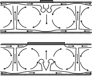
Figure 1. The fluid loop model and two partially insulated fluid loop models. (a) The fluid loop model for a convection cell of width L and height d (modified from Turcotte & Oxburgh (Reference Turcotte and Oxburgh1967), and Grigné, Labrosse & Tackley (Reference Grigné, Labrosse and Tackley2005)). (b) The partially insulated fluid loop model for stagnant mode I (SM I). (c) The partially insulated fluid loop model for stagnant mode II (SM II). The lower panels of (a)–(c) are the simplified velocity profiles of the corresponding models.
For an uninsulated convection cell (W = 0), the upper and lower boundaries of the convection cell are considered to be perfectly symmetrical to each other, as are the cold and the hot thermal plumes (figure 1a). By symmetry, the core temperature of the convection cell is given by  ${T_i} = {\textstyle{1 \over 2}}({T_0} + {T_1})$, and thus the top and the bottom heat fluxes are equal to each other (Qs = Qb). For a convection cell at steady state, the conservation of energy dictates that the heat flux at the bottom must be transported by the thermal plumes to the top surface. Therefore, each of the half-plumes carries half of the heat flux, i.e.
 \begin{equation}{A_c} = {A_h} = {\textstyle{1 \over 2}}{Q_b} = {\textstyle{1 \over 2}}{Q_s},\end{equation}
where Ac and Ah are the heat rate carried by half of the cold and the hot plumes, respectively,
 \begin{gather}{A_h} = \rho {C_p}v\delta ({T_h} - {T_i}),\end{gather}
 \begin{gather}{A_c} = \rho {C_p}v\delta ({T_i} - {T_c}).\end{gather}
Here, v and δ are the mean vertical velocity and the mean width of the half-plume, respectively; Th and Tc are the mean temperature of the hot and the cold plumes, respectively.
A steady state also entails that the heat flux into the fluid from the bottom equals that out of the fluid from the top, and therefore the internal temperature of the cell, Ti, remains constant with time. Nevertheless, this balance is easily disturbed if an adiabatic plate suddenly lingers over the top of the cell (figure 1b,c), which is the case of SM I and SM II (Mao Reference Mao2021). During SM I/II, the convergent/divergent flow underneath the plate results in a small net flow velocity and therefore a stagnant plate. The stagnant adiabatic plate shortens the distance of cooling at the top. Therefore, the heat flux into the cell from the bottom is larger than that out of the cell from the top, i.e. Qb > Qs. Energy conservation dictates that this excess of heat flux must be transferred into the interior and heats up the internal fluid, raising its temperature by ΔTi over a time interval of Δt
 \begin{equation}\rho {c_p}\Delta {T_i}(L - \delta )d = ({Q_b} - {Q_s})\Delta t.\end{equation}
Here, δ represents the half-width of the plume uncovered by the plate, corresponding to the hot plume for SM I (figure 1b) and the cold plume for SM II (figure 1c). This uncovered plume forms as a natural outcome of TBL instability and it contacts directly with the upper and lower TBL, similar to the no-plate cases. Therefore, its temperature remains relatively constant. Subtracting its half-width  $\delta $ from the cell length L yields the length
  $(L - \delta )$ over which temperature will increase. Multiplying
  $L - \delta$ by the fluid depth d results in the volume,
  $(L - \delta )d$, per unit length parallel to the roll axis.
Substituting (2.4) and (2.5) into (2.9) and assuming an infinitesimal time Δt, the time derivative of the internal (core) temperature of the convection cell is obtained
 \begin{equation}\frac{{\partial {T_i}}}{{\partial t}} = \frac{{\Delta {T_i}}}{{\Delta t}} = \frac{2}{{(L - \delta )d}}{\left( {\frac{\kappa }{{\rm \pi} }} \right)^{1/2}}\left[ {({T_1} - {T_i}){L^{1/2}} - ({T_i} - {T_0}){{\left( {L - \frac{W}{2}} \right)}^{1/2}}} \right]{u^{1/2}}.\end{equation}
As heat accumulates underneath the plate, the internal temperature Ti gradually increases. This increase in Ti results in a variation of the cell length and flow speed, as demonstrated later. Therefore, the partial insulation turns the classic loop model, which quantifies the steady-state flow of a single convection cell, into a model that evolves with time.
The buoyant forces of the half-cold and the half-hot plume, denoted as fc and fh, respectively, can be expressed as
 \begin{gather}{f_c} = \alpha \rho g\delta d({T_i} - {T_c}),\end{gather}
 \begin{gather}{f_h} = \alpha \rho g\delta d({T_h} - {T_i}).\end{gather}
Here, the symbols α, ρ, g denote the thermal expansion coefficient, the reference density and the gravitational acceleration, respectively.
The fluid loop model focuses on the magnitude of the maximum flow velocity within the convection cell, instead of the detailed velocity variation within it. Therefore, a simplified velocity profile is adopted for the large-scale flow (figure 1a): the upper and lower layers of the cell are of zero vertical velocity and the horizontal velocity does not vary with the horizontal position x, but only with the vertical position y, peaking at the top and the bottom boundaries and diminishing linearly to zero at the middle depth; similarity, the viscous layers of the plume is of zero horizontal velocity and the vertical velocity does not vary with y, but only with x, peaking at the axis of the plume and diminishing linearly to zero at a distance of λ away from the axis. With this simplified velocity profile, the upper/lower layer is associated with only the horizontal shear, whereas the viscous layer of the plume is associated only with the vertical shear. The horizontal and vertical shear stresses, τh and τv, are expressed respectively as
 \begin{gather}{\tau _h} = \mu \left( {\frac{{\partial u}}{{\partial z}}} \right) = \mu \frac{{2u}}{d},\end{gather}
 \begin{gather}{\tau _v} = \mu \left( {\frac{{\partial v}}{{\partial x}}} \right) = \mu \frac{v}{\lambda },\end{gather}
where μ is the dynamic viscosity of the fluid; u and v are, respectively, the maximum horizontal and the maximum vertical speeds within the convection cell; λ is the width of the layer subject to the viscous shear of the half-plume (figure 1).
The simplified velocity profiles are a good approximation when the width of the convection cell is much larger than the total width of the two half-plumes (i.e.  $L \gg 2\lambda$) and the considered region is far away from the corners of the cell. Nevertheless, in the corner regions, the flow turns around. In this case, flow velocity varies strongly with both x and y, the simplified velocity profiles no longer apply nor the shear stresses derived from it. Therefore, in the application of the loop model, one needs to be cautious when the corner regions constitute a large portion of the convection cell, since the validity of the result is expected to deteriorate as the portion increases.
Mass conservation dictates that the horizontal mass flux in the cell equals the vertical one, and therefore a relation between u and v is established as
 \begin{equation}u\frac{d}{2} = v\lambda .\end{equation}
2.2. Stagnant mode I
SM I is the stagnant mode of a small plate over a cold downwelling (Mao Reference Mao2021). When a small plate encounters the cold downwelling at its leading edge, it is soon stopped by the associated impeding flow and enters into a long duration of stagnancy as it straddles the convergent flow underneath. The stagnant plate switches the boundary condition underneath from isothermal cooling to an adiabatic condition (figure 1b). In the loop model, the two convection cells underneath the plate are idealized to be perfectly symmetrical to each other with each covered by half of the plate. Therefore, with the arrival of the plate, the cooling distance at the top of the convection cell is suddenly shortened from L to L − W/2. In this case, the fluid parcel falls down from the top boundary layer without being sufficiently cooled as in the uncovered case, and therefore temperature of the cold downwelling underneath the plate increases.
In contrast, the hot plume, uncovered by the plate, contacts directly with the upper and the lower TBLs, similar to the no-plate cases. Therefore, its temperature (Th) should remain relatively constant. Similar to the no-plate case with a cell length of L − W/2, the heat flux transported by the half-hot plume to the top boundary equals half of the top heat flux Qs. An equilibrium between (2.7) and half of Qs in (2.4) yields
 \begin{equation}\delta ({T_h} - {T_i}) = \kappa ({T_i} - {T_0})\frac{u}{v}{\left( {\frac{{L - \frac{W}{2}}}{{u{\rm \pi} \kappa }}} \right)^{1/2}}.\end{equation}
Substituting (2.15) and (2.16) into (2.12), the buoyant force of the half-hot plume is expressed as
 \begin{equation}{f_h} = 2\lambda \alpha \rho g\kappa ({T_i} - {T_0}){\left( {\frac{{L - \frac{W}{2}}}{{u{\rm \pi} \kappa }}} \right)^{1/2}}.\end{equation}
The work of the driving force (the buoyant force of the half-hot plume) equals the work of the associated resisting force (the viscous shear force)
 \begin{equation}{f_h}v = {\tau _v}\,dv + {\tau _h}Lu.\end{equation}
Here, the left side ( fh  $v$) represents the work of the buoyant force per unit time. The right side is a combination of the work of the shear force imposed on the uprising plume
  $({\tau _v}\,dv)$ and on the associated horizontal flow in the upper layer (τhLu) per unit time. Assuming a unit length in the roll axis of the convection cell, the multiplication of τv by d, and τh by L transfers the shear stresses to shear forces.
Substituting (2.13), (2.14), (2.15), (2.17) into (2.18), yields the expression for the horizontal velocity u
 \begin{equation}u = \frac{\kappa }{d}{\left( {\frac{{Ra}}{{2\sqrt {\rm \pi} }}} \right)^{2/3}}{\left( {\frac{{{T_i} - {T_0}}}{{{T_1} - {T_0}}}} \right)^{2/3}}\frac{{{{\left[ {{{\left( {L - \frac{W}{2}} \right)} / d}} \right]}^{1/3}}}}{{{{\left( {\frac{L}{d} + \frac{{{d^3}}}{{8{\lambda^3}}}} \right)}^{2/3}}}},\end{equation}
where Ra is the Rayleigh number defined as
 \begin{equation}Ra = \frac{{\rho g\alpha ({T_1} - {T_0}){d^3}}}{{\mu \kappa }}.\end{equation}
Substituting (2.15) and (2.19) back into (2.16) yields a relation between the core temperature Ti and the cell length L
 \begin{align}\delta ({T_h} - {T_i}) = {2^{4/3}}\lambda ({T_i} - {T_0}){\left( {\frac{{{T_i} - {T_0}}}{{{T_1} - {T_0}}}} \right)^{ - 1/3}}{({\rm \pi} \,Ra)^{ - 1/3}}{\left( {\frac{{L - \frac{W}{2}}}{d}} \right)^{1/3}}{\left( {\frac{L}{d} + \frac{{{d^3}}}{{8{\lambda^3}}}} \right)^{1/3}}.\end{align}
A derivative of (2.21) with respect to time t yields a relation between ∂L/∂t and ∂Ti/∂t
 \begin{align}\frac{{\partial
L}}{{\partial t}} ={-} \frac{{1 + \frac{{{2^{4/3}}}}{\delta
}\lambda {{({\rm \pi} \,Ra)}^{ - 1/3}}{{({T_1} -
{T_0})}^{1/3}}\frac{2}{3}{{({T_i} - {T_0})}^{ -
1/3}}{{\left( {\frac{{L - \frac{W}{2}}}{d}}
\right)}^{1/3}}{{\left( {\frac{L}{d} +
\frac{{{d^3}}}{{8{\lambda^3}}}}
\right)}^{1/3}}}}{\begin{array}{l}\frac{{{2^{4/3}}}}{\delta }\lambda
{{({\rm \pi} \,Ra)}^{ - 1/3}}{{({T_1} -
{T_0})}^{1/3}}\frac{1}{{3d}}{{({T_i} - {T_0})}^{2/3}}\\\quad \times\left[
{{{\left( {\frac{{L - \frac{W}{2}}}{d}} \right)}^{ -
2/3}}{{\left( {\frac{L}{d} +
\frac{{{d^3}}}{{8{\lambda^3}}}} \right)}^{1/3}} + {{\left(
{\frac{{L - \frac{W}{2}}}{d}} \right)}^{1/3}}{{\left(
{\frac{L}{d} + \frac{{{d^3}}}{{8{\lambda^3}}}} \right)}^{ -
2/3}}} \right]\end{array}}\frac{{\partial {T_i}}}{{\partial
t}}.\end{align}
\begin{align}\frac{{\partial
L}}{{\partial t}} ={-} \frac{{1 + \frac{{{2^{4/3}}}}{\delta
}\lambda {{({\rm \pi} \,Ra)}^{ - 1/3}}{{({T_1} -
{T_0})}^{1/3}}\frac{2}{3}{{({T_i} - {T_0})}^{ -
1/3}}{{\left( {\frac{{L - \frac{W}{2}}}{d}}
\right)}^{1/3}}{{\left( {\frac{L}{d} +
\frac{{{d^3}}}{{8{\lambda^3}}}}
\right)}^{1/3}}}}{\begin{array}{l}\frac{{{2^{4/3}}}}{\delta }\lambda
{{({\rm \pi} \,Ra)}^{ - 1/3}}{{({T_1} -
{T_0})}^{1/3}}\frac{1}{{3d}}{{({T_i} - {T_0})}^{2/3}}\\\quad \times\left[
{{{\left( {\frac{{L - \frac{W}{2}}}{d}} \right)}^{ -
2/3}}{{\left( {\frac{L}{d} +
\frac{{{d^3}}}{{8{\lambda^3}}}} \right)}^{1/3}} + {{\left(
{\frac{{L - \frac{W}{2}}}{d}} \right)}^{1/3}}{{\left(
{\frac{L}{d} + \frac{{{d^3}}}{{8{\lambda^3}}}} \right)}^{ -
2/3}}} \right]\end{array}}\frac{{\partial {T_i}}}{{\partial
t}}.\end{align}
Since L > W/2, it is clear from (2.22) that the sign of ∂L/∂t is opposite to that of ∂Ti/∂t. This suggests that, as heat accumulates underneath the plate, an increase of the core temperature Ti leads to a decrease of the cell length L, that is, a shrinkage of the convection cell underneath the plate. This shrinkage is reasonable physically. Since an increase of the core temperature Ti leads to a decrease of the buoyant force fh of the hot plume (2.12), which is the driving force of the convection cell, a decreased driving force is expected to propel the fluid to a shorter distance and thus sustain a smaller convection cell.
This predicted shrinkage has indeed been observed in results of numerical simulation for SM I (Mao et al. Reference Mao, Zhong and Zhang2019; Mao Reference Mao2021), in which the shrinkage is embodied by the migration of the two neighbouring hot plumes towards the plate. Here, through the partially insulated loop model, a further step is made to quantify this plume motion towards the plate. This will be achieved in § 4 through an integrated analysis of (2.10), (2.19), (2.22) and the model prediction will be verified by results of full numerical simulation.
2.3. Stagnant mode II
A similar analysis can be carried out for SM II, in which case the stagnant plate quickly nurtures a hot upwelling underneath and lingers over it (figure 2b). The end of the hot upwelling touches the adiabatic plate, instead of the cooling surface, and therefore this upwelling is not being sufficiently cooled as in the no-plate cases. Heat accumulates underneath the plate and temperature of the hot upwelling increases with time. In contrast, the cold plume, uncovered by the plate, contacts directly with the upper and the lower TBLs, similar to the no-plate case. Therefore, its temperature is not much affected by the insulating plate, i.e. Tc remains relatively constant. Accordingly, the heat flux carried by the half-cold plume to the bottom boundary still equals half of the bottom heat flux, i.e. 0.5Qb. Therefore, an equilibrium between (2.8) and half of Qb in (2.5) yields
 \begin{equation}\delta ({T_i} - {T_c}) = \kappa ({T_1} - {T_i})\frac{u}{w}{\left( {\frac{L}{{u{\rm \pi} \kappa }}} \right)^{1/2}}.\end{equation}
Following the same process specified in SM I, the counterparts of (2.17)–(2.19), (2.21), (2.22), which apply to SM I, can be derived for SM II, which are (2.24)–(2.28), respectively. The buoyant force of the half-cold plume, fc, is
 \begin{equation}{f_c} = 2\lambda \alpha \rho g({T_1} - {T_i}){\left( {\frac{{\kappa L}}{{u{\rm \pi} }}} \right)^{1/2}}.\end{equation}
A balance between the work of the driving force (the buoyant force) and that of the resisting force (the viscous shear force) yields
 \begin{equation}{f_c}v = {\tau _v}\,dv + {\tau _h}Lu.\end{equation}
Here, the right side is a combination of the work of the shear force imposed on the downfalling plume  $({\tau _v}\,dv)$ and the associated horizontal flow in the lower layer (τhLu) per unit time. The horizontal velocity, u, of the convection cell is
 \begin{equation}u = \frac{\kappa }{d}{\left( {\frac{{Ra}}{{2\sqrt {\rm \pi} }}} \right)^{2/3}}{\left( {\frac{{{T_1} - {T_i}}}{{{T_1} - {T_0}}}} \right)^{2/3}}\frac{{{{(L/d)}^{1/3}}}}{{{{\left( {\frac{L}{d} + \frac{{{d^3}}}{{8{\lambda^3}}}} \right)}^{2/3}}}}.\end{equation}
The internal temperature Ti is related to the length of the convection cell L by
 \begin{equation}\delta ({T_i} - {T_c}) = {2^{4/3}}\lambda ({T_1} - {T_i}){\left( {\frac{{{T_1} - {T_i}}}{{{T_1} - {T_0}}}} \right)^{ - 1/3}}{({\rm \pi} \,Ra)^{ - 1/3}}{\left( {\frac{L}{d}} \right)^{1/3}}{\left( {\frac{L}{d} + \frac{{{d^3}}}{{8{\lambda^3}}}} \right)^{1/3}}.\end{equation}
Accordingly, the relation between  $\partial L/\partial t$ and
 $\partial {T_i}/\partial t$ is
 \begin{align}\frac{{\partial
L}}{{\partial t}} = \frac{{\left( {1 +
\frac{{{2^{4/3}}}}{\delta }\lambda {{({T_1} -
{T_0})}^{1/3}}{{({\rm \pi} \,Ra)}^{ -
1/3}}\frac{2}{3}{{\left( {\frac{L}{d}}
\right)}^{1/3}}{{\left( {\frac{L}{d} +
\frac{{{d^3}}}{{8{\lambda^3}}}} \right)}^{1/3}}{{({T_1} -
{T_i})}^{ - 1/3}}} \right)}}{\begin{array}{l}\frac{{{2^{4/3}}}}{\delta
}\lambda {{({T_1} - {T_0})}^{1/3}}{{({\rm \pi} \,Ra)}^{
- 1/3}}\frac{1}{{3d}}{{({T_1} - {T_i})}^{2/3}}\\\quad \times\left(
{{{\left( {\frac{L}{d}} \right)}^{ - 2/3}}{{\left(
{\frac{L}{d} + \frac{{{d^3}}}{{8{\lambda^3}}}}
\right)}^{1/3}} + {{\left( {\frac{L}{d}}
\right)}^{1/3}}{{\left( {\frac{L}{d} +
\frac{{{d^3}}}{{8{\lambda^3}}}} \right)}^{ - 2/3}}}
\right)\end{array}}\frac{{\partial {T_i}}}{{\partial
t}}.\end{align}
\begin{align}\frac{{\partial
L}}{{\partial t}} = \frac{{\left( {1 +
\frac{{{2^{4/3}}}}{\delta }\lambda {{({T_1} -
{T_0})}^{1/3}}{{({\rm \pi} \,Ra)}^{ -
1/3}}\frac{2}{3}{{\left( {\frac{L}{d}}
\right)}^{1/3}}{{\left( {\frac{L}{d} +
\frac{{{d^3}}}{{8{\lambda^3}}}} \right)}^{1/3}}{{({T_1} -
{T_i})}^{ - 1/3}}} \right)}}{\begin{array}{l}\frac{{{2^{4/3}}}}{\delta
}\lambda {{({T_1} - {T_0})}^{1/3}}{{({\rm \pi} \,Ra)}^{
- 1/3}}\frac{1}{{3d}}{{({T_1} - {T_i})}^{2/3}}\\\quad \times\left(
{{{\left( {\frac{L}{d}} \right)}^{ - 2/3}}{{\left(
{\frac{L}{d} + \frac{{{d^3}}}{{8{\lambda^3}}}}
\right)}^{1/3}} + {{\left( {\frac{L}{d}}
\right)}^{1/3}}{{\left( {\frac{L}{d} +
\frac{{{d^3}}}{{8{\lambda^3}}}} \right)}^{ - 2/3}}}
\right)\end{array}}\frac{{\partial {T_i}}}{{\partial
t}}.\end{align}

Figure 2. The migration of neighbouring hot plumes toward the plate in SM I. (a–g) Snapshots of the temperature field and streamlines showing the evolution of the underlying flow structure with time. The dotted and solid black lines represent streamlines of clockwise and anti-clockwise flows, respectively, with an interval of 800. The black triangles at the bottom of (b–f) denote the horizontal position of the identified hot plume for SM I. Snapshots (b–f) are at equal time intervals. (h) Time series of plate speed up, the average temperature T of fluid underlying the plate, the average normal stress σyy at plate bottom. The horizontal dashed lines in (h) mark the corresponding time of the snapshots of (a–g).
Contrary to SM I, where the sign of  $\partial L/\partial t$ is opposite to that of
  $\partial {T_i}/\partial t$, (2.28) shows that these two terms are of the same sign in SM II. Therefore, as heat accumulates in the underlying convection cells (Ti increases), the cells are expected to expand (L increases) in the form of cold plumes moving away from the plate. This expansion is physically reasonable, since (2.11) shows that an increase of Ti leads to an increase of the buoyant force of the cold plume, which is the driving force of the convection cell. An increased driving force is expected to propel the fluid to a longer distance and therefore sustain a larger convection cell.
This predicted expansion has indeed been observed in the results of numerical simulation for SM II, in which the neighbouring cold plumes are observed to move away from the plate (Mao et al. Reference Mao, Zhong and Zhang2019; Mao Reference Mao2021). In § 4, the motion of the cold plumes predicted by the loop model will be verified by results of full numerical simulation.
3. Model configuration and methods for numerical simulation
The model configuration and methods for numerical simulation have been detailed in Mao (Reference Mao2021) and therefore are only briefly introduced here for completeness. A simplified 2-D domain of aspect ratio eight is considered. A freely floating plate is introduced on top of the fluid, with the width W ranging from 0.25 to 5 (normalized by the fluid depth d). Simplifications used in previous studies (for example, Gurnis Reference Gurnis1988; Whitehead & Behn Reference Whitehead and Behn2015; Mao et al. Reference Mao, Zhong and Zhang2019; Mao Reference Mao2021) are also incorporated here: a uniform viscosity, the Boussinesq approximation and the dropping of the inertia and advection terms in the momentum equation owing to the large Prandtl number of the mantle. This simplified model extracts the thermal blanket effect of a continent from the complex system of the Earth and focuses on the thermally induced fluid–structure interaction. The dimensionless governing equations in a Cartesian coordinate system are
 \begin{gather}\frac{{\partial {u_i}}}{{\partial {x_i}}} = 0,\end{gather}
 \begin{gather}\frac{{{\partial ^\textrm{2}}{u_i}}}{{\partial {x_j}\partial {x_j}}} = Ra\frac{{\partial P}}{{\partial {x_i}}} - Ra{\delta _{i2}}T,\end{gather}
 \begin{gather}\frac{{\partial T}}{{\partial t}} + {u_j}\frac{{\partial T}}{{\partial {x_j}}} = \frac{{{\partial ^2}T}}{{\partial {x_j}\partial {x_j}}},\end{gather}
where x 1 and x 2 represent the horizontal and vertical coordinates, respectively, and u 1 and u 2 denote the horizontal and vertical velocity components, respectively. This indicial notation is used only in the governing equations (3.1)–(3.3) and is substituted elsewhere by the basic Cartesian notion for simplicity, where x = x 1, y = x 2 and u = u 1, v = u 2. The symbols t, P, T represent time, pressure and temperature, respectively, and δij denotes the Kronecker delta. Equations (3.1)–(3.3) are made dimensionless using the length scale d, the velocity scale κ/d, the temperature (relative to the top boundary temperature T 0) scale (T 1 − T 0) and the pressure gradient scale  $\rho g\beta ({T_1} - {T_0})$, where ρ is the fluid density. The value of Ra is set to be 5 × 10⁷ for all the following simulations
The fluid is initially isothermal (T = 1) and stationary. The bottom of the fluid (y = 1) is set to be isothermal (T = 1) and a sudden cooling (T = 0) is imposed at the top surface (y = 0) except the plate–fluid interface, which is set to be adiabatic  $(\partial T/\partial y = 0)$, a simplified extreme condition to highlight the thermal blanket effect of a continent. The vertical boundaries of the fluid domain are set to be periodic, allowing the fluid/plate to flow/move out of one side and into the other, a better approximation to the Earth than the rigid-wall condition adopted in previous studies (Whitehead & Behn Reference Whitehead and Behn2015; Mao et al. Reference Mao, Zhong and Zhang2019). A stress-free condition is set for the top and the bottom boundaries of the fluid, except the plate–fluid interface, which is set to be no slip, i.e. the flow velocity at the interface is the same as the plate velocity. Similar to previous studies (Mao et al. Reference Mao, Zhong and Zhang2019; Mao Reference Mao2021), the plate velocity is determined by averaging the flow velocity at the first grid cell below the interface. This method was first used by Gable, O'Connell & Travis (Reference Gable, O'Connell and Travis1991) and it ensures that the net horizontal shear force exerted by the flow on the plate is zero and therefore energy is conserved in the convecting system.
The governing equations are advanced numerically in time using the finite-volume method. The code has been validated when solving natural convection problems (for example, Mao, Lei & Patterson Reference Mao, Lei and Patterson2009, Reference Mao, Lei and Patterson2010). The semi-implicit method for pressure-linked equations scheme (Patankar Reference Patankar1980) and the quadratic upstream interpolation for convective kinematics scheme (Leonard Reference Leonard1979) are adopted for pressure–velocity coupling and spatial derivative approximation, respectively. According to the mesh and time-step dependency test detailed in Mao (Reference Mao2021), an equidistant mesh of 2000 × 250 is selected with a time step of 6 × 10⁻⁸.
4. The thermal blanket effect on plume motion
Previous studies (Mao et al. Reference Mao, Zhong and Zhang2019; Mao Reference Mao2021) have shown that, as plate size increases, its motion transitions from long-term stagnancy over cold downwelling (SM I) to short-term stagnancy over hot upwelling (SM II), and eventually to a unidirectional motion with no stagnancy. During SM I, the thermal blanket effect is embodied by the gradual migration of neighbouring hot plumes toward the stagnant plate and the weakening of cold downwelling underneath the plate (Mao Reference Mao2021). As plate size increases, SM II emerges, in which case the enhanced thermal blanket effect is reflected by the fast growth of hot upwelling underneath the plate and the associated moving of neighbouring cold plumes away from the plate (Mao Reference Mao2021). These observed plume motions have been quantified in § 2 through the analysis on partially insulated loop models. The model prediction will be compared here with the numerical results.
4.1. Hot plumes toward the plate in SM I
The migration of neighbouring hot plumes towards the plate during SM I is first tracked in the results of full numerical simulation and then compared with predications from the loop model. For the loop model, the initial condition and parameter (δ and λ) values are ascertained from the results of numerical simulation.
4.1.1. Results of numerical simulation
Initially, a small plate (W = 0.5) drifts along with a coherent underlying flow (figure 2a). When it encounters a cold downwelling and the associated impeding flow at its leading edge, it soon stops and enters into a stagnant mode, i.e. SM I. In this case, the plate straddles the convergent horizontal flow associated with the cold downwelling (figure 2b). Similar to a ball on a concave surface, any motion away from the balanced position will be inhibited by an opposing force and therefore the plate is stably trapped. During its lingering over the cold downwelling (figure 2b–f), the plate accumulates heat underneath, illustrated by the increasing average temperature of the underlying fluid (figure 2h). Meanwhile, the thermal blanket effect is also embodied by the gradual weakening of the cold downwelling, and the gradual migration of neighbouring hot plumes toward the plate (figure 2b–f). As a result, the underlying convection cells gradually shrink and eventually vanish when the hot plumes arrive at the plate (figure 2b–g). Accompanying the arrival of hot plumes, the plate soon shifts to one of the large convection cells and exhibits a velocity burst (figure 2g), temporarily terminating SM I.
The horizontal positions of the neighbouring hot plumes are tracked over this stagnant duration. With a storage of the simulation results each 40 time steps, 2166 snapshots are saved and analysed over a stagnant duration of 5.2 × 10⁻³. Unlike the ideal plume shape assumed in the loop model (figure 1), the shape of the real plume is quite irregular, often associated with significant inclination or diverted branches. This irregularity poses a challenge to an objective and consistent identification of the plume position. However, scrutiny of the evolution of the plumes suggests that, although the shape of the plume evolves with time, the position of its root is relatively stable (figure 3). Therefore, for each snapshot, the root of the hot plume is identified from the vertically averaged temperature profile over a thin bottom layer of thickness 0.032, as marked by the red triangles in the right panels of figure 3(a–g). This thickness is close to the average thickness of the TBL (0.036), which will be derived later. A slight variation of this thickness does not affect the results.

Figure 3. The evolution of hot plume with time in SM I. (a–g) Left panel: snapshots of the temperature field and streamlines zooming in on the flow domain near the plate; right panel: the corresponding temperature profile averaged over a thin bottom layer of thickness 0.032. The red triangles and dashed lines mark the position of the hot plume. The blue dashed lines trace the position of the neighbouring hot thermals that gradually move to the hot plume. (h) The distance from plate centre to the adjacent hot plume, on the left side (Ll) and on the right side (Lr). (i) The maximum horizontal speed |u| at the bottom of the left (|u|l) and the right (|u|r) convection cells.
Figure 3 zooms in on half of the flow domain with snapshots of the temperature field and streamlines on the left and the corresponding profiles of vertically averaged temperature over the thin bottom layer on the right. Apart from the hot plume, shorter blobs of warm fluid are observed to rise up from the bottom (figure 3). These blobs of warm fluid are referred to as thermals (Howard Reference Howard1966; Sparrow, Husar & Goldstein Reference Sparrow, Husar and Goldstein1970; Chu & Goldstein Reference Chu and Goldstein1973; Griffiths Reference Griffiths1986). Their formation is a manifestation of local instability and is related to fluctuations of local velocity. The positions of these thermals are traced by the blue dashed lines (the right panels of figure 3) over time. In the presence of a large-scale horizontal flow within the convection cell, hot thermals are observed to migrate along with the large-scale flow toward the neighbouring hot plume (from figure 3a–e for the left plume, from figure 3a–d for the right plume) and grow in length on their way. Accompanied by this migration and growth, the maximum horizontal speed |u| at the bottom gradually increases (figure 3i), peaking at the moment when the thermals at the bottom just coalesce with the plume. This suggests that a more centralized thermal anomaly, or a stronger plume, generates a higher momentum for the convection cell.
Over the duration from figure 3(e–g), no new thermal is observed to move to the left plume and its thermal anomaly gradually weakens. This results in a decreasing maximum horizontal speed |u| for the associated convection cell (figure 3i, blue line from e to g). For the right plume, although hot thermals are moving to it (from figure 3d–g), they still remain relatively far away from the plume, and the top part of the thermals becomes separated as the bottom part moves fast ahead (figure 3g). The weakening of the thermal anomaly of the right plume (from figure 3d–g) is also accompanied by a decrease of |u| for the associated convection cell (figure 3i, orange line from d to g). These results show that the maximum horizontal flow speed |u| fluctuates with the thermal anomaly of the plume, peaking at times when neighbouring thermals just coalesce with the plume and gradually decreasing afterwards until another set of thermals approaches the plume.
Owing to the presence of these hot thermals, more than one peak appears in the temperature profile near the plume position (right panel of figure 3a–g). This poses a challenge to an automatic identification of the plume position from these peaks. However, a scrutiny suggests that a distinct feature that differentiates the plume-induced peak from the thermal-induced peak is their horizontal speed. Consecutive snapshots show that the thermals are moving fast to the plume. As traced by the blue lines in figure 3, their speed can reach up to 1.8 × 10⁴, of the same order of magnitude as the maximum flow speed. In contrast, the plume is rather stationary. Over the duration from figure 2(b–f) (4.89 × 10⁻³), the distance between the two neighbouring hot plumes shrinks from 3.25 to 0.92. This translates to an average migration speed of 476, a magnitude almost two orders smaller than the migration speed of the thermals. As traced by the red lines and triangles (figure 3), the plumes are indeed rather stationary compared with the thermals. Therefore, apart from being shorter and not penetrating to the top surface, another feature that differentiates thermals from plumes is the migration speed. While the plume is rather stationary, the thermals are migrating fast with the large-scale flow toward the plume.
An automatic identification method is adopted to trace the evolution of plume position during SM I. First, the initial position of the neighbouring hot plumes is identified through an integration of the initial temperature profile and the corresponding snapshot. In the initial temperature profile, the position of the plume-induced peak is identified as the initial plume position. Since the plume is rather stationary over the short interval (2.4 × 10⁻⁶) between each saved snapshot, once its initial position is ascertained, its subsequent position can be automatically determined by identifying the peak that is closest to the peak identified one time interval earlier. This method is objective and consistent, and automatically excludes the fast moving thermal-induced peaks. It ensures that no abrupt change of plume position occurs between each time interval and that the variation of plume position is a smooth process. The identified plume distance away from the plate centre is indeed rather smooth over the short period shown in figure 3(h).
The plume position is tracked over a much longer duration (figure 4a), along with the corresponding maximum horizontal speed from the plate centre to the nearest hot plumes (figure 4b). As predicted by the partially insulated loop model in § 2 (2.22), the distance between neighbouring hot plumes shrinks with time (figure 4a). Accompanying this shrinkage is the decrease of the maximum horizontal speed |u| (figure 4b). On top of a long-term decreasing trend, the simulation results of |u| also fluctuate strongly with time since |u| is sensitive to local velocity pulses, peaking at times when thermals just coalesce with the hot plume and strengthen its thermal anomaly (figure 3).

Figure 4. Evolution of the plume distance (L) and the maximum horizontal speed |u| during SM I. (a) The distance of the left and right plumes away from the plate centre, denoted as Ll and Lr, respectively. Here, Ll + Lr denotes the distance between the two plumes. (b) The maximum horizontal speed |u| at the bottom from the plate centre to the nearest hot plume on the left side (|u|l) and on the right side (|u|r). ‘NS’ denotes results from full numerical simulation, ‘Model’ denotes theoretical prediction from the partially insulated loop model. The vertical dashed lines and the cyan dots mark, respectively, the corresponding time and the values of L and |u| for snapshots shown in figure 2(b–f).
4.1.2. The partially insulated loop model
To derive the evolution of plume position from the partially insulated loop model for SM I, (2.10), (2.19) and (2.22) are written as a function of time and also in non-dimensional forms to facilitate a direct comparison with the non-dimensional results from numerical simulation
 \begin{equation}\frac{{\partial {T_i}(t)}}{{\partial t}} = \frac{{2u{{(t)}^{1/2}}}}{{{{\rm \pi} ^{1/2}}(L(t) - \delta )}}\left[ {({T_1} - {T_i}(t)){L^{1/2}} - ({T_i}(t) - {T_0}){{\left( {L(t) - \frac{W}{2}} \right)}^{1/2}}} \right],\end{equation}
 \begin{equation}u(t) = {\left( {\frac{{Ra}}{{2\sqrt {\rm \pi} }}} \right)^{2/3}}{({T_i}(t) - {T_0})^{2/3}}\frac{{{{\left( {L(t) - \frac{W}{2}} \right)}^{1/3}}}}{{{{\left( {L(t) + \frac{1}{{8{\lambda^3}}}} \right)}^{2/3}}}},\end{equation}
 \begin{equation}\frac{{\partial L(t)}}{{\partial t}} ={-} \frac{{{{({\rm \pi} \,Ra)}^{1/3}}\left[ {1 + \frac{{{2^{7/3}}}}{{3\delta }}\lambda {{({\rm \pi} \,Ra)}^{ - 1/3}}{{({T_i}(t) - {T_0})}^{ - 1/3}}{{\left( {L(t) - \frac{W}{2}} \right)}^{1/3}}{{\left( {L(t) + \frac{1}{{8{\lambda^3}}}} \right)}^{1/3}}} \right]\frac{{\partial {T_i}(t)}}{{\partial t}}}}{{\frac{{{2^{4/3}}}}{{3\delta }}\lambda {{({T_i}(t) - {T_0})}^{2/3}}\left[ {{{\left( {L(t) - \frac{W}{2}} \right)}^{ - 2/3}}{{\left( {L(t) + \frac{1}{{8{\lambda^3}}}} \right)}^{1/3}} + {{\left( {L(t) - \frac{W}{2}} \right)}^{1/3}}{{\left( {L(t) + \frac{1}{{8{\lambda^3}}}} \right)}^{ - 2/3}}} \right]}}.\end{equation}
All the variables in the above equations are non-dimensionalized using the same scales as those used for the non-dimensional governing equations (3.1)–(3.3). Equations (4.1)–(4.3) show that the internal temperature Ti(t), the horizontal flow speed u(t), and the distance of plume away from the plate centre L(t) are interrelated variables. This coupled set of equations governs the evolution of temperature, flow speed and plume distance with time.
An appropriate initial condition has to be set before advancing equations (4.1)–(4.3) in time. The initial values of the core temperature Ti and the cell length L are determined from the numerical results (Ti = 0.505, L = 1.624) at the time when SM I just starts (figure 2b). In the partially insulated loop model (figure 1b), the two idealized perfectly symmetrical convection cells shrink at the same rate. In reality, these two convection cells are not symmetrical (figure 2b). In this case, simulation results show that the hot plume further away from the plate moves at a faster rate toward the plate than the nearer plume (figure 4a). Eventually, the two plumes arrive near the edge of the plate at roughly the same time, similar to the symmetrical case. The initial distances of the left and the right plumes away from plate centre are obtained from the simulation results (figure 2b, left plume Ll = 1.200; right plume Lr = 2.048) and their average (1.624) is used as the initial value of L for the partially insulated loop model.
Meanwhile, the values of δ and λ in (4.1)–(4.3), denoting the thickness of the thermal and the viscous layers of the half-plume respectively, are also obtained from the simulation results. At the root of the hot plume, the hot TBL turns 90° to form the plume. Since very little conduction can occur during this turning, the thermal layer thickness of the half-hot plume, δ, should be the same as the thickness of the TBL. To obtain the average thickness of the TBL, the vertical distribution of temperature for each snapshot is obtained by horizontally averaging the temperature at each vertical position. All the profiles during SM I are then averaged and shown in figure 5(a). From this vertical profile, a thickness of 0.036 is obtained for both the upper and the lower TBLs and the value also remains the same for cases with different plate widths (0.5 and 2).

Figure 5. The thickness of the TBL and the thermal layer of the plume. (a) The vertical temperature profiles averaged over the stagnant duration, the horizontal dashed lines mark the boundary of the TBL where the temperature reaches the maximum for the upper layer and the minimum for the lower layer. The symbol δ denotes the thickness of the TBL, which remains the same (0.036) for cases with different plate widths (0.5 and 2.0), and is also the same for the upper and the lower TBLs. (b) A zoom in on a sub-region of figure 2(b) where a rather regular straight hot plume is present. The red line shows the corresponding vertically averaged temperature  $\bar{T}$. The two black dashed lines mark the edge of the hot plume where the temperature reaches a local minimum. The distance between these two lines is 0.072, exactly twice the thickness of the TBL.
Unlike the idealized regular and straight plume assumed in the loop model, a realistic plume is often irregular, inclined and associated with diverted branches (figure 2). The inclination and diverted branches result in a broader signal of the plume in the vertically averaged temperature profile than the idealized regular plume. Therefore, for a direct estimation of the thermal layer thickness of an idealized plume, a relatively straight plume with no evident diverted branch along its stem is selected (figure 5b). The thermal layer thickness of the plume (2δ) deduced from the distance between the two local minima in the temperature profile (figure 5b) is 0.072. This is exactly twice the average thickness of the TBL shown in figure 5(a). Therefore, as expected, the thermal layer thickness of the half-plume is well represented by the thickness of the TBL and thus the value of 0.036 is used for δ.
For the evaluation of λ, the strongest plume with the highest vertical speed is selected in each snapshot. Compared with a weak plume, a strong plume has a velocity profile less susceptible to local velocity pulses, and therefore better represented by the linear velocity profile in the loop model. With a maximum vertical speed of |v|max and a linearly decreasing profile, the average vertical speed of the strongest half-plume is then |v|max/2. Mass conservation entails that the vertical flow rate should equal the horizontal flow rate
 \begin{equation}\frac{{|v{|_{\max }}}}{2}{\lambda _e} = \overline{|u|}\frac{d}{2},\end{equation}
where  $\overline{|u|}$ denotes the corresponding average horizontal speed over the depth, and λe denotes the effective viscous layer thickness of the plume. By obtaining the values of |v|max and the corresponding
  $\overline{|u|}$ for each snapshot, the time series of λe are derived from (4.4) (figure 6a). Subject to local velocity pulses, the value of λe fluctuates with time and therefore differs from the theoretical λ value for the idealized plume in the loop model. Nevertheless, the mean of λe, which is 0.351, provides a good estimation for λ.

Figure 6. The thickness (λ) of the layer subject to the viscous shear of the half-plume. (a) The maximum vertical speed |v|max within the domain (blue line), the maximum of the vertically averaged horizontal speed  $\overline{|u|}$ within the adjacent cells (orange line) and the effective value of λ (black line), denoted as λe. The mean of λe (the red dashed line) is 0.351. (b) A zoom in on a sub-region of figure 2(c) where a strong hot plume is present, with an almost symmetrical distribution of the vertical velocity near the centre of the plume. The red line shows the average vertical velocity
  $\bar{v}$ over the depth. The two black lines mark the positions where
  $\bar{v}$ changes sign, the distance (2λ) between which represents the viscous layer thickness of the plume. The obtained viscous layer thickness of the half-plume is λ = 0.348, close to the mean of λe.
For a direct evaluation of λ, the vertical velocity profile of a strong plume is analysed (figure 6b). For the idealized plume in the loop model, the vertical velocity decreases linearly, from the maximum at the plume axis to zero at a distance of λ away from the axis (figure 1b). In reality, the hot plume is often associated with adjacent thermals moving toward it (figure 3). These uprising thermals boost the local vertical velocity and therefore hinder its decrease with distance away from the plume axis. As a result, the linearly decreasing velocity profile is distorted and the velocity decreases to zero at a larger distance than the theoretical value. Therefore, in order to obtain the theoretical value of λ from the simulation results, the effect of uprising thermals should be excluded and thus a strong hot plume with no adjacent uprising thermals is selected from the snapshots (figure 6b). The width of the viscous layer of the plume (2λ) is deduced from the distance between neighbouring positions where the vertical velocity decreases to zero. The obtained λ value (0.348) is less than 1 % different from the average λe (0.351) (figure 6a). Therefore, the results of these methods are consistent and 0.351 is used for λ in the following calculation.
As a further verification, with the above estimated value of λ, the thickness of the TBL, δ, can be determined from the loop model and compared with the value estimated from the numerical results. For a convection cell of unit width (L = 1) with no plate (W = 0), its internal temperature Ti reaches the average temperature of the top (T 0 = 0) and the bottom (T 1 = 1) boundaries, i.e. Ti = 0.5, at steady state. The non-dimensional velocity u of this cell is estimated from (4.2) and then substituted back into the non-dimensional form of (2.2), from which the temperature field is obtained. The corresponding isotherms show the presence of an evident TBL (figure 7a). Temperature T increases away from zero at the top boundary and approaches a constant value of 0.5 (figure 7b). The lower boundary of the TBL is deemed as where T increases to 99 % of Ti − T 0, i.e. 0.5, and thus it corresponds to the isotherm of T = 0.0495, shown by the red contour at the outer edge (figure 7a). For the considered domain of a unit width (L = 1), the thickness of the TBL, δ, increases with x and reaches a maximum of 0.036 at x = 1, the same as that obtained from the numerical results (figure 5a). Varying the cell width L from 0.8 to 1.2, the maximum value of δ varies less than 3.4 %. This consistency further validates the loop model, in particular the consistency between the λ value and the δ value.

Figure 7. The thickness of the TBL δ predicted by the loop model (a) isotherms at an interval of 0.005 calculated from the non-dimensional form of (2.2). The isotherms near the top are so densely distributed that they form colour bands and are indiscernible, signifying a large vertical gradient. The red line at the outer edge marks where the temperature reaches 0.495, which is 99 % of Ti − T 0, i.e. the temperature difference between the interior and the top surface. (b) The vertical temperature profiles at different x. The red dashed lines mark where the temperature reaches 99 % of Ti − T 0, representing the thickness of local TBL. This thickness increases with x.
After the initial conditions and the values of δ and λ are ascertained, the differential forms of (4.1)–(4.3) are advanced in time with the same time step (6 × 10⁻⁸) as that used in the full numerical simulation. Results from the loop model are shown together with the results from numerical simulation in figure 4. Since the two underlying convection cells in the loop model are perfectly symmetrical to each other, only one of the cells is analysed. The distance between the two plumes is calculated as 2L. Similarly, the sum of the maximum horizontal speeds of the left and the right cells is calculated as 2u.
Not subject to fluctuations of the local flow, results from the loop model show a smooth long-term variation purely induced by the thermal blanket effect, which agrees well with the long-term trend of the simulation results (figure 4). Both results show a similar duration of plume migration toward the plate (figure 4a). Accompanying this migration, the underlying convection cells shrink and their maximum horizontal speed |u| decreases (figure 4b). Subject to local velocity pulses, the simulation result of |u| fluctuates strongly with time, peaking at times when the adjacent hot plume is strong (e.g. marked by the left triangle in figure 3e). Nevertheless, its long-term variation trend agrees well with the prediction of the loop model (figure 4b). Therefore, the partially insulated loop model successfully predicts the evolution of flow structure during SM I.
An evident trend in figure 4(a) is that the agreement between the model prediction and the simulation results deteriorates as the sum of cell width Ll + Lr decreases below 2, a value relatively close to 4λ (≈1.4), which is the total width of the four half-plumes contained in these two convection cells. In this case, the corner regions where the flow turns around dominate the convection cell. As discussed previously, in these corner regions, the simplified velocity profile is no longer representative, and therefore larger deviation is expected between the model prediction and the simulation results.
Further, the no-slip plate–fluid interface dictates that flow velocity there is almost zero. This differs significantly from the simplified velocity profile which assumes a maximum speed at the top surface. Accordingly, the shear stress based on the simplified velocity profile no longer applies there. For SM I, the shear stress of the upper layer is involved in the loop model (2.18). In case when  $L \gg W/2$, the interface constitutes only a small fraction of the top surface and therefore does not cause significant discrepancy. As L decreases and the no-slip interface begins to dominate the top surface, apart from the corner regions, the no-slip interface is another factor that leads to the discrepancy between the model prediction and the simulation results (figure 4a). The scenario is different for SM II, which involves the shear stress of the lower layer (2.25), instead of the upper layer. For the lower layer, with a stress-free bottom boundary, its velocity profile is not affected by the no-slip interface. Therefore, for SM II, the no-slip interface is not expected to affect the accuracy of model prediction.
4.2. The moving of cold plumes away from the plate in SM II
As the plate becomes larger, SM I transitions into SM II, in which the enhanced thermal blanket effect enables the stagnant plate to nurture hot upwelling underneath it. Accompanying the strengthening of the underlying upwelling, the neighbouring cold plumes move gradually away from the plate (Mao Reference Mao2021). This migration of the cold plume is tracked in the simulation results and compared with predictions from the loop model.
4.2.1. Results of numerical simulation
When a medium sized plate (W = 2) encounters a strong downwelling and the associated impeding flow at its leading edge (figure 8a), it slows down. This slowing down extends from the no-slip plate–fluid interface to the interior of the fluid through the viscous drag. As a result, the horizontal mass transport underneath the plate decreases and can no longer balance the vertical transport of the adjacent hot plume behind the plate. In this case, mass conservation entails the formation of a cold downwelling near the trailing edge to divert the horizontal flow brought up by the hot plume (figure 8b). This newly formed cold plume blocks the momentum supply from the adjacent hot plume to the plate and thus the plate is no longer being propelled and becomes stagnant.

Figure 8. The moving of neighbouring cold plumes away from the plate in SM II. (a–f) Snapshots of the temperature field and streamlines showing the evolution of underlying flow structure with time. The dotted and solid black lines represent streamlines of clockwise and anti-clockwise flows, respectively, with an interval of 800. The black triangles at the top of (c–f) denote the horizontal positions of the identified cold plume for SM II. Snapshots (c–f) are at an equal time interval. (h) Time series of plate speed up, the average temperature T of fluid underlying the plate, the average normal stress σyy at plate bottom.
Meanwhile, the slowdown of the insulating plate leads to a more pronounced thermal blanket effect. Instead of gradually attracting adjacent hot plumes toward it as in SM I, the enhanced thermal blanket effect of a larger plate enables it to accumulate heat by directly nurturing thermals underneath it. As these thermals grow and hit the bottom of the plate, the vertical normal stress (σyy) there switches from positive (extensional) to negative (compressional) (figure 8h). As heat accumulates underneath, the average temperature of the underlying fluid increases (figure 8h). Accompanying this increase is the migration of adjacent cold plumes away from the plate (figure 8c–f). As cold plumes move far away, the plate becomes unstable since any disturbances away from the balanced position will be magnified rather than inhibited, analogous to a ball on a convex. Therefore, the plate soon moves onto one of the convection cells and resumes its speed (figure 8g).
The distances of the adjacent cold plumes away from the plate centre are tracked using the automatic tracking method described in § 4.1.1 over the stagnant duration. Results show that the plume distance increases relatively smoothly over the stagnant duration (figure 9a). In contrast, the maximum horizontal speed |u| of the underlying convection cells fluctuates strongly with time (figure 9b), owing to its sensitivity to local velocity pulses. Similar to SM I, the simulation results of |u| fluctuate with the thermal anomaly of the plume. The strong thermal anomaly of the left cold plume in figure 8(d,f) (marked by the left triangle) corresponds to a local peak in the time series of |u|l (figure 9b), whereas the weak left cold plume in figure 8(e) corresponds to a low value of |u|l (figure 9b).

Figure 9. Evolution of the plume distance (Ll, Lr) and the maximum horizontal speed |u| during SM II. (a) The distance of the left and right cold plumes away from the plate centre, denoted as Ll and Lr, respectively. Here, Ll + Lr denotes the distance between the two cold plumes. (b) The maximum horizontal speed |u| at the bottom from the plate centre to the nearest cold plume on the left side (|u|l) and on the right side (u|r). ‘NS’ denotes results from full numerical simulations, ‘Model’ denotes theoretical prediction from the partially insulated loop Model. The vertical dashed line and the cyan dots mark the time and the corresponding values for snapshots shown in figure 8(c–f).
4.2.2. The partially insulated loop model
For SM II, (2.10), (2.26) and (2.28) compose the set of equations that govern the evolution of convection cells underneath the plate. These equations are reformulated as a function of time and in non-dimensional forms. Equation (2.10) transfers to (4.1), and (2.26) and (2.28) become, respectively,
 \begin{equation}u(t) = {\left( {\frac{{Ra}}{{2\sqrt {\rm \pi} }}} \right)^{2/3}}{\left( {\frac{{{T_1} - {T_i}(t)}}{{{T_1} - {T_0}}}} \right)^{2/3}}\frac{{L{{(t)}^{1/3}}}}{{{{\left( {L(t) + \frac{1}{{8{\lambda^3}}}} \right)}^{2/3}}}},\end{equation}
 \begin{equation}\frac{{\partial L(t)}}{{\partial t}} = \frac{{{{({\rm \pi} \,Ra)}^{1/3}} + \frac{{{2^{7/3}}}}{{3\delta }}\lambda L{{(t)}^{1/3}}{{\left( {L(t) + \frac{1}{{8{\lambda^3}}}} \right)}^{1/3}}{{({T_1} - {T_i}(t))}^{ - 1/3}}}}{{\frac{{{2^{4/3}}}}{{3\delta }}\lambda {{({T_1} - {T_i}(t))}^{2/3}}\left[ {L{{(t)}^{ - 2/3}}{{\left( {L(t) + \frac{1}{{8{\lambda^3}}}} \right)}^{1/3}} + L{{(t )}^{1/3}}{{\left( {L(t) + \frac{1}{{8{\lambda^3}}}} \right)}^{ - 2/3}}} \right]}}\frac{{\partial {T_i}(t)}}{{\partial t}}.\end{equation}
The evolution of plume distance L and flow speed u can be derived by advancing the differential forms of these equations in time. Similar to the case of SM I, the initial values of plume distance (L = 1.108) and internal temperature (Ti = 0.571) are obtained directly from the simulation results (figure 8c). For the value of δ, it has been confirmed in § 4.1 that δ is well represented by the average thickness of the TBL. The average TBL thickness for the case of W = 2.0 is revealed to be same as that for the case of W = 0.5 (figure 5a). Therefore, the same value of 0.036 is adopted for δ here. Since the thermal layer thickness of the plume, δ, does not change with plate width, it is expected that the viscous layer thickness of the plume, λ, remains the same. In fact, using the method described in § 4.1, which is based on (4.4), time series of the effective value of λ are obtained with a mean of 0.352, only slightly different from the value (0.351) for the case of W = 0.5. No discernible difference is observed between the results using these two different values.
Using the above initial conditions and parameter values, (4.1), (4.5) and (4.6) are advanced in time with a time step of 6 × 10⁻⁸, the same as the time step of numerical simulation. The evolution of plume distance (distance between the two adjacent cold plumes) predicted by the loop model agrees well with the results of full numerical simulation (figure 9a). The magnitude of the maximum horizontal speed |u| revealed by the loop model is also in overall agreement with that obtained from numerical simulation (figure 9b). Since the loop model does not consider local velocity pulses, it predicts a smooth increase of |u| with time. In contrast, the simulation results of |u| fluctuate with the thermal anomaly of the local plume, as discussed in § 4.2.1. Compared with the duration of SM I for the case of W = 0.5, the duration of SM II for the case of W = 2 is much shorter and this prevents a comparison of the long-term trend between model predictions and simulation results. Overall, the loop model successfully predicates the evolution of plume distance L and flow speed during SM II, showing a smooth variation not subject to fluctuations of the local flow, but induced purely by the thermal blanket effect.
5. The emergence of a unidirectionally moving plate
Simulation results show that, irrespective of plate size, plate velocity always peaks at times when the plate overlies a single convection cell, with a strong hot upwelling near its trailing edge and a cold downwelling ahead of it (figures 2a, 8a and 10a). In these cases, the strong hot upwelling brings up a strong horizontal flow that propels the plate. To simplify, this strong hot upwelling adjacent to the trailing edge is termed the ‘propelling’ upwelling hereafter. As the plate encounters the cold downwelling at its leading edge, the associated impeding flow slows it down. For SM I, the horizontal flow brought up by the original ‘propelling’ upwelling is fully counteracted by the opposing flow (figure 2b). For SM II, it is blocked by a newly formed cold plume near the trailing edge and therefore can no longer reach the plate (figure 8b). In both cases, a new ‘propelling’ upwelling has to be established for the plate to resume its motion.

Figure 10. The unidirectional moving mode shown with the case of W = 3, in which no stagnation or reversal of the plate is observed. (a–e) Snapshots of the temperature field and streamlines showing the evolution of underlying flow structure with time. The dotted and solid black lines represent streamlines of clockwise and anti-clockwise flows, respectively, with an interval of 800. (h) Time series of plate speed up, the average temperature T of fluid underlying the plate, the average normal stress σyy at plate bottom.
Since the thermal blanket effect is enhanced with plate size, it is expected that the time it takes to establish a new ‘propelling’ upwelling decreases with plate size. For a small plate in SM I, a long duration is required. In this case, the neighbouring hot plumes migrate slowly toward the plate. Their arrival at the plate and subsequent coalescence generates the new ‘propelling’ plume that boosts plate motion. As plate size increases, SM II emerges, in which the enhanced thermal blanket effect enables the plate to directly nurture hot thermals underneath it. Within a short time, the hot thermals grow into a strong ‘propelling’ upwelling that boosts plate motion. It is expected that, as plate size continues to increase, the enhanced thermal blanket effect will eventually enable the plate to establish a new ‘propelling’ upwelling before it is fully stopped by the impeding flow ahead. In this case, the plate will no longer stop and will move unidirectionally.
Such a unidirectionally moving mode is indeed observed for the case with a plate width of  $W = 3$ (figure 10). Initially, the plate overlies a strong horizontal flow brought up by the ‘propelling’ upwelling and moves fast (figure 10a). Although it slows down as it encounters the impeding flow (figure 10b), its strong thermal blanket effect becomes prominent with this slowdown. A group of hot thermals is soon nurtured underneath it (figure 10c), growing into a strong upwelling that pushes the cold downwelling and the associated impeding flow ahead (figure 10d). As a result, the plate resumes its fast motion (figure 10e). In this case, the thermal blanket effect is so strong that a new hot ‘propelling’ upwelling is established before the plate is fully stopped. Therefore, no stagnation or reversal occurs. The plate moves unidirectionally.
Time series of plate speed |up| show that as plate size increases, its motion becomes increasingly persistent (or less likely to reverse), transitioning to a unidirectional motion at  $W = 3$ (figure 11a). Meanwhile, plate speed |up| transitions from highly concentrated on low values (stagnant) to a more scattered distribution and eventually to an increasingly concentrated distribution on a relatively high value, which suggests an increasingly stable motion (figure 11b). A small plate of W = 0.5 exhibits long durations of stagnancy (low |up|) interrupted by episodic velocity bursts (spikes of |up|) (figure 11a). As plate size increases, the duration of stagnancy (the time interval between neighbouring velocity spikes) decreases. This suggests that an enhancing thermal blanket effect with plate size enables an increasingly fast generation of new hot ‘propelling’ upwelling which boosts plate motion after it is slowed down. As a result, the plate becomes less likely to be stagnant and more persistent in its motion.

Figure 11. Plate speed |up| and its probability density distribution for cases with different plate size W. (a) Time series of plate speed, the blue and orange lines represent positive and negative plate velocity up, respectively. (b) Probability density distribution of plate speed |up|.
For a more quantitative evaluation of the time interval between neighbouring spikes, spectrum analysis is conducted on the time series of plate speed (figure 12). The dominant frequency fd increases with plate size W, jumping abruptly at W = 0.75 and then increasing linearly with W up to W = 3, after which the increasing rate slows down (figure 12). The abrupt jump at W = 0.75 corresponds to the transition of the dominant modes, from SM I to SM II. The slowdown of the increasing rate of fd for W > 3 is a manifestation of the finite size effect. It is observed that, when plate motion is being boosted by the newly nurtured hot thermals, the underlying convection cells expand, to a width much larger than the plate width (figure 10c–e). This expansion pushes the cold downwelling and the associated impeding flow away from the plate and leads to an increase in plate speed. Nevertheless, for large plate cases of W > 3, the limited size of the flow domain confines the expansion of the underlying convection cells. This confinement in turn hinders the boosting of plate motion, which is reflected in the slowdown of the increase of fd with W.

Figure 12. Spectra and the dominant frequencies of the time series of plate speed |up| for cases with different plate widths W. (a) Spectra of the time series of |up|, the red lines mark the dominant frequency fd with the highest amplitude. (b) The dominant frequencies fd versus plate width W. The black line is the result of the linear least squares fitting, fd = 239.77W + 394.97 for 0.75 ≤ W ≤ 3. The pink, blue and orange zones highlight the scope of W for SM I, SM II and the UMM, respectively.
An increase of the dominant frequency with plate size means a decrease of the dominant period, or a decreased time interval between large velocity spikes, consistent with the trend shown in the time series of |up| (figure 11a). Therefore, the increase of fd with plate size suggests that the enhanced thermal blanket effect with plate size enables an increasingly fast feedback between the slowdown of the plate and the generation of new hot ‘propelling’ upwelling which boosts plate motion. When the feedback is so fast that a new ‘propelling’ upwelling is established to boost plate motion before the plate is fully stopped, the UMM emerges. Therefore, the critical condition for the emergence of UMM is that the time required for the plate to stop after encountering an impeding flow is longer than that required for its motion to be boosted by newly generated upwelling.
These two times are compared for two cases of different plate widths (figure 13). For the small plate case of W = 0.5 for which SM I dominates, the plate is fully stopped and enters into a long duration of stagnation before its motion is boosted (figure 13a). Therefore, the time required for the impeding flow to fully stop the plate, denoted by ts, is much smaller than the half-dominant period T/2, as sketched in figure 13(c). In contrast, for the large plate case of W = 3 for which the plate moves unidirectionally, plate motion is boosted before it is fully stopped (figure 13b). In this case, ts is larger than T/2, as sketched in figure 13(d). For this large plate case, T/2 represents the time at which plate speed starts to rise after encountering the impeding flow.

Figure 13. Time series of plate speed |up| over a dominant period, and the corresponding sketches that focus on the contrast between the plate stop time ts and the half-period T/2. (a) Time series of |up| for W = 0.5. (b) Time series of |up| for W = 3. (c) A sketch of the time series over a dominant period for the small plate cases for which stagnancy occurs, i.e. the plate stops before its motion is boosted, ts < T/2 (d) A sketch of the time series over a dominant period for the large plate cases for which no stagnancy occurs, i.e. plate motion is boosted before the plate is stopped, ts > T/2.
The above analysis suggests that the emergence of UMM can be predicted by comparing the value of ts with that of T/2. If ts > T/2, then plate motion is boosted before it stops, and thus UMM occurs. The critical plate size for the emergence of UMM is where these two values (ts and T/2) intersect. The half-dominant period T/2 can be directly derived from the dominant period fd. For the value of ts, a simplified model is established, which focuses on the slowdown of a plate by the impeding flow.
With the no-slip interface adopted here, the plate does not move onto the cold downwelling and the impeding flow. In fact, during the process of slowing down, the cold downwelling is always observed at the leading edge of the plate (e.g. figure 10b), dipping toward the plate. This dipping brings an impeding flow underneath the leading edge of the plate, which imposes a resisting shear force to the moving plate and therefore gradually slows it down. This slowing down is then passed down from the no-slip interface to the interior of the fluid through viscous shear, resulting in the decrease of flow speed underneath the plate.
Focusing on the slowdown of the plate, this 2-D process is simplified by a 1-D model at the plate–fluid interface. Featuring the constant presence of an opposing flow at the leading edge of the plate during the slowdown process, an opposing flow with a speed of u 0 is assumed at the leading edge. The plate, moving with a speed of up(t) at time t, makes an infinitesimal intrusion (up(t)Δt) onto this opposing flow over an infinitesimal time of Δt. Since plate velocity embodies the net velocity of the underlying flow, this intrusion decreases the plate velocity at time  $t + \Delta t$, which is expressed as
 \begin{equation}{u_p}(t + \Delta t) = \frac{{{u_p}(t)(W - {u_p}(t)\Delta t) - {u_0}{u_p}(t)\Delta t}}{W}.\end{equation}
Here, the speed of the opposing flow, u 0, is taken as the average flow speed at the top surface. This value is obtained from the results of numerical simulation for different plate widths (figure 14a). It decreases with plate width W up to W = 2 and then levels off up to W = 5. This value is also taken as the initial plate speed up just before encountering the impeding flow. By advancing equation (5.1) in time, the decreasing of plate speed up with time can be derived. Results show that, as plate size increases, it takes longer for the plate to stop, i.e. ts increases with plate width W (figure 14b); whereas, it takes a shorter time for plate motion to be boosted after being slowed down, since the dominant period T (the inverse of fd) decreases with W. Therefore, the plate moves more persistently and is less likely to be stopped as its size increases.

Figure 14. (a) The average flow speed u 0 at the top surface. (b) The decrease of plate speed up with time derived from (5.1) for cases with different plate widths W.
To determine the stop time ts from the results of this simplified model (figure 14b), a criterion has to be set to judge the stopping of the plate. Theoretically, the plate is stopped as its speed |up| decreases to zero. In reality, plate speed fluctuates with the flow speed. Therefore, the standard deviation of flow speed, representing the amplitude of its fluctuation, is deemed as the criterion for the stop of the plate. The time that the plate speed |up| decreases to this value is deemed as the stop time ts.
The derived stop time ts is compared with the half-dominant period T/2 for cases with different plate widths (figure 15a). A linear interpolation shows that these two values intersect at a critical plate width of Wc = 2.79. For a very small plate of  $W \ll {W_c}$,
  ${t_s} \ll T/2$, i.e. the time it takes for the impeding flow to stop the plate is much shorter than that takes for the thermal blanket effect to boost its motion. Therefore stagnancy occurs, accompanied by a large number of reversal events (figure 15b). For these cases, the thermal blanket effect is not sufficiently strong to establish a new ‘propelling’ hot upwelling to overwhelm the impeding flow before the plate stops. As plate size increases, ts increases, whereas T/2 decreases. These two values gradually approach each other, intersecting at a critical width of Wc. Accompanying this approach is the decrease of reversal events (figure 15b), suggesting an increasingly persistent plate motion. For large plates of W > Wc, ts > T/2, plate motion is boosted before it stops, and therefore the plate moves unidirectionally with no stagnancy or reversal (figure 15b). In these cases, the sufficiently large size endows the plate with a sufficiently strong heat-accumulating ability to timely generate hot ‘propelling’ upwelling to boost its motion before it is fully stopped by the impeding flow. The predicted critical plate width (Wc = 2.79) for the UMM agrees well with results of full numerical simulation, since the number of plate reversal events indeed vanishes somewhere between W = 2.5 and W = 3.0 (figure 15b). Further, it is also in excellent agreement with the critical plate width (2.78) derived previously using another method (Mao Reference Mao2021).

Figure 15. (a) A comparison of the stop time ts (orange line) and the half-dominant period T/2 (blue line) for cases with different plate widths W. The dashed line marks the switch between ts < T/2 and ts > T/2, the corresponding plate width Wc (2.79) is the critical width for UMM. The pink, blue and orange zones mark the range of plate width for cases dominated by SM I, SM II and UMM, respectively (b) The number of plate reversal events over a non-dimensional duration of 0.1 obtained from numerical simulation results for cases with different plate widths W, approaching zero as W increases to Wc.
Both methods adopt the same simplified slowdown model to derive the evolution of plate speed after encountering the impeding flow. In addition to the slowdown model, the previous method (Mao Reference Mao2021) also includes a plume-chasing model. These two models are integrated in the previous study to estimate the time it takes for the hot plume to reach the trailing edge of the plate after the plate is slowing down, and compared with the time when plate speed decreases to half its initial value. In the case where the former is larger than the latter, mass conservation dictates that a cold downwelling will form at the trailing edge and the plate will stop. This is in fact another way to compare the response time of the flow with the slowdown time of the plate, analogous to the comparison of T/2 with ts in the present study.
6. Discussions and conclusions
6.1. The motion of adjacent plumes during SM I and SM II
Plates of different sizes exhibit quite different behaviour when encountering impeding flow at their leading edge. A small plate (W ≤ 0.5) is easily stopped and enters into a long-term stagnancy above cold downwelling (SM I). In this case, the relatively weak thermal blanket effect is manifested by the gradual moving of the neighbouring hot plumes towards the plate. As the thermal blanket effect is enhanced with plate size, the heat accumulation transitions from a gradual attraction of existing hot plumes to a direct nurturing of new hot thermals underneath. As a result, another stagnant mode (SM II) emerges at W = 0.75, in which case, the stopped plate enters into a short-term stagnancy above the newly generated hot upwelling. During this mode, the hot upwelling underneath becomes increasingly strong, pushing the adjacent cold plumes away from the plate and resulting in an expansion of the underlying convection cells.
These migrations of plumes, i.e. hot plumes towards the plate in SM I and cold plumes away from the plate in SM II, have been revealed in previous studies (Mao et al. Reference Mao, Zhong and Zhang2019; Mao Reference Mao2021). The present study further quantifies these plume motions and reveals their underlying mechanism through analysis on a partially insulated loop model with an adiabatic plate–fluid interface. Compared with the classic loop model, which characterises the steady-state flow of a single convection cell, the introduction of an adiabatic plate–fluid interface turns the model into a model for an unsteady-state flow. Being partially insulated at the top surface, the heat flux into the cell from the bottom is larger than that out of the cell from the top. This excess of heat gradually warms up the interior of the convection cell, lowering/raising the temperature difference between hot/cold plume and the internal fluid. Since the buoyant force of the plume is proportional to this temperature difference, the increase in the internal temperature results in the decrease/increase of the buoyant force of the hot/cold plume with time.
For SM I, the plate lingers over cold downwelling. Being directly covered by the plate, the cold downwelling gradually warms up and its thermal and momentum characteristics are altered correspondingly, no longer the cold plume in the loop model. In contrast, the adjacent hot plume, not directly insulated by the plate, maintains its characteristics and its buoyancy force drives the convective circulation. As the internal temperature Ti increases with time, the buoyant force of the hot plume decreases. The decreased buoyant force (driving force) propels the fluid to a shorter distance and therefore sustains a smaller convection cell. As a result, the underlying convection cells shrink, with the adjacent hot plumes gradually moving toward the plate. The contrary applies to the case of SM II. In SM II, the buoyant force of the adjacent cold plume increases with an increasing Ti. The increased driving force propels the fluid to a longer distance and therefore sustains a larger convection cell. As a result, the underlying convection cells expand, with the adjacent cold plumes moving away from the plate.
These plume migrations in SMs I and II are analysed in their respective partially insulated loop model. Through an integrated analysis based on the equilibrium between the work of the driving force (buoyant force) and that of the resisting force (viscous force), and the mass and the energy conservation, the evolution of plume position and the horizontal flow speed are derived from the model, which are well validated by results of full numerical simulation.
6.2. The emergence of a UMM
At each encounter of an impeding flow at its leading edge, the plate slows down. This slowdown results in a more pronounced thermal blanket effect, i.e. its ability to accumulate heat underneath. The enhancing of the thermal blanket effect with plate size enables an increasingly fast feedback between the slowdown of a plate and the strengthening of hot upwelling which boosts plate motion. As a result, as plate size increases, plate motion becomes increasingly persistent (less likely to reverse), eventually transferring to a UMM; the time interval between neighbouring velocity spikes becomes increasingly short. Correspondingly, the dominant frequency fd of plate speed increases with plate width W, with an abrupt jump at a plate width of W = 0.75, followed by a linear increase up to W = 3. The abrupt jump at W = 0.75 corresponds to the transition of coupling modes from SM I to SM II. As the finite size effect emerges for W ≥ 4, the increase of fd with W slows down. Overall, the dominant frequency of plate speed quantifies the variation of thermal blanket effect with plate size.
The critical condition for the emergence of the UMM is that plate speed starts to rise before it is fully stopped by the impeding flow. For large plates that move unidirectionally, plate speed starts to rise roughly at half the dominant period (T/2) after being slowed down. The time it takes for an impeding flow to stop the plate, ts, estimated from a simplified model, is compared with the half-dominant period T/2 for cases of different plate widths. Results show that it takes longer to stop a larger plate, i.e. ts increases with plate width. In contrast, T/2 decreases with plate width. These two values intersect at a critical plate width of Wc = 2.79. For large plate cases of W > Wc, the UMM emerges, in which case the plate moves unidirectionally with no stagnancy or reversal. The predicted critical plate width for the UMM agrees well with results of full numerical simulation and with the previous result (Mao Reference Mao2021).
6.3. Implication for the real Earth
6.3.1. Continent–mantle coupling
Previous studies (Mao et al. Reference Mao, Zhong and Zhang2019; Mao Reference Mao2021) have demonstrated the similarity of the revealed coupling modes to some real cases of continent–mantle coupling. SM I, SM II and the UMM have been related to the current coupling status of the continents of Zealandia, Africa and Eurasia, respectively. The predicted underlying thermal structure, and the normal and shear stresses at the interface found good expression in real Earth cases. To lay the context for the later discussion on plume motion, these real Earth cases are briefly summarized here.
The small continent of Zealandia, predicted to have probably experienced long terms of stagnancy over cold downwelling, has indeed been straddling the oceanic subduction (downwelling) site at the Pacific-Australia plate boundary since its arrival there 25 million years ago (Sutherland Reference Sutherland1999; Cande & Stock Reference Cande and Stock2004). The vertical extensional normal stress (positive σyy, figure 2h) exerted by the downwelling is expected to drag Zealandia downwards. Indeed, over 90 % of Zealandia is submerged under water (Suggate, Stevens & te Punga Reference Suggate, Stevens and te Punga1978). Further, the Southern Alps there is a surface expression of the horizontal compressional shear stress exerted by the underlying convergent flow associated with the cold downwelling.
In contrast, the much larger continent of Africa, predicted to probably be stagnant over hot upwelling, has indeed been roughly stationary since the break-up of Pangaea (Burk & Torsvik Reference Burk and Torsvik2004; Torsvik et al. Reference Torsvik, Steinberger, Cocks and Burke2008, Reference Torsvik, Burke, Steinberger, Webb and Ashwal2010) and is indeed being uplifted by a huge mantle plume in its southern and eastern parts (Ebinger & Sleep Reference Ebinger and Sleep1998; Ritsema, van Heijst & Woodhouse Reference Ritsema, van Heijst and Woodhouse1999). The vertical compressional normal stress (negative σyy, figure 8h) exerted by the plume on the continent is expected to lift the continent up. Indeed, southern and eastern Africa stand more than 1 km above sea level, which is twice the elevation of a normal craton (Lithgow-Bertelloni & Silver Reference Lithgow-Bertelloni and Silver1998). Further, the large fracture zones exemplified by the Great Rift Valley in eastern Africa are surface expressions of the horizontal extensional shear stress exerted by the underlying divergent flow associated with the hot upwelling.
The even larger continent of Eurasia, predicted to move unidirectionally, has indeed not been reported to be stagnant or to have reversed direction by itself. Simulation results suggest that the UMM is characterized by the presence of a hot plume near the trailing edge of the plate and a cold downwelling near the leading edge, possibly dipping toward the plate. As the Eurasia plate is moving toward the Pacific plate, these predicted thermal structures are indeed embodied, respectively, by the hot plume underneath the Africa continent and the subducted cold oceanic slabs dipping toward the Eurasian plate at its leading edge (Kao & Rau Reference Kao and Rau1999; Shiomi, Sato & Obara Reference Shiomi, Sato and Obara2004).
6.3.2. Continent speed
Time series show that plate speed fluctuates strongly with time, especially for small plates (figure 11). This is reasonable since small plates are more susceptible to velocity pulses induced by local flow. The speed of small plates during velocity bursts can reach up to ~1.6 × 10⁴ (figure 11). Using a thermal diffusivity of  $\kappa$ = 10−6, and a mantle depth of d = 2880 km (Turcotte & Schubert Reference Turcotte and Schubert2002), this non-dimensional speed transfers to a dimensional value of 17.5 cm y−1. Such a large magnitude of speed has indeed been observed in real continents of the Earth. The relatively small continent of India, although it is currently moving with a speed of approximately 5.8 cm y−1 (Argus, Gordon & DeMets Reference Argus, Gordon and DeMets2011), indeed experienced a velocity burst of ~15 cm y−1 in the late Cretaceous during its separation from the Africa plate (Peirce Reference Peirce1978; Schult & Gordon Reference Schult and Gordon1984; Acton Reference Acton1999). In contrast to this velocity burst, the large Eurasian plate, currently encountering a cold subducting slab (downwelling) at its leading edge (analogous to figure 10b), is expected to be being slowed down by the associated impeding flow. Simulation results show that, although a large plate exhibits a relatively steady unidirectional motion, during the slowdown stage, an impeding flow can slow its speed down to ~2 × 10³ (figure 11a,b). Although even lower values are observed, the probability is low. This value (
 $2\times10^{3}$) transfers to a dimensional value of 2.2 cm y−1, which is close to the current speed of the Eurasia plate (Argus et al. Reference Argus, Gordon and DeMets2011).
6.3.3. Plume motion
The geological community hold that the deep mantle plume and the associated hot spots are relatively stationary. Therefore, they are adopted as the reference points for deriving the relative velocity of the floating plates (Burk & Torsvik Reference Burk and Torsvik2004; Torsvik et al. Reference Torsvik, Steinberger, Cocks and Burke2008, Reference Torsvik, Burke, Steinberger, Webb and Ashwal2010). For example, the north-westward motion of the pacific plate over a rather stationary mantle plume results in the formation of the Hawaiian-Emperor chain of volcanic islands. The speed of the pacific plate can be estimated by dividing the distance between neighbouring islands by the difference between their rock ages. As to why these volcanic islands are not continuous, but isolated, the quasi-periodic strengthening and weakening of the hot plume revealed by results of numerical simulation may give us a hint (figure 3). Results show that neighbouring short thermals at the bottom move towards the hot plume and then coalesce with it (figure 3). The strength of the hot plume peaks at this coalescence and gradually weakens afterwards, until another set of newly nurtured short thermals approach the hot plume. This fluctuation in plume strength may lead to the discontinuity of the volcanic islands, since a stronger hot plume is more likely to break through the oceanic lithosphere and form volcanic islands, whereas a weaker plume is less likely to leave a mark on the Earth's surface.
Consistent with the assumption of the geologic community, the migration speed of the hot plume towards the plate in SM I is indeed small. From figure 2b–f, the distance between the two neighbouring hot plumes shortens a non-dimensional length of 2.33 over a duration of 4.89 × 10⁻³. The average speed of a single plume is then 238, which transfers to a dimensional value of 2.6 mm y−1, an order of magnitude smaller than the current average speed of the continents. However, this average value must be taken cautiously. Both the results from numerical simulation and those from the loop model suggest that the speed of the hot plume towards the plate is not constant, but varying with its distance to the plate (figure 4a). Results from the loop model show that the plume migration speed initiates at approximately 220, levelling off for a while, and increases noticeably as the plume becomes close to the plate, with a peak of 490, equivalent to 5.4 mm y−1. Although this peak value is still small, this plume motion is non-negligible compared with the stagnant plate which is trapped in SM I.
In contrast to the normal case of a plate being propelled by the horizontal flow brought up by a rather stationary hot plume, in this case, it is the other way around. A rather stagnant plate is constantly attracting neighbouring hot plumes toward it through its thermal blanket effect. A rather stagnant plate and a constantly moving hot plume may be counter-intuitive at first sight. Nevertheless, it is the counter-intuitiveness of this phenomenon that highlights the significance of the thermal blanket effect of the continental plates. The thermal blanket effect enables a two-way feedback between the plate and the plume. As a result, instead of being a passive drifter, a stagnant insulating plate can induce a constant motion of its neighbouring plumes. Although the relatively large size of the present continents dictates the rareness of SM I in the current Earth, with the continent of Zealandia being an example, SM I is expected to be much more prevalent in the early days of the Earth when continents just started to form and therefore were still small. In those days, the significance of SM I and the associated plate-ward motion of the hot plumes are expected to be much more pronounced.
Further, in the early days, owing to the presence of much more abundant radioactive elements, the internal heating rate due to radioactive decay is much higher. For example, its value in the early Hadean period (approximately 4.5 billion years before the present) is five times the present value (Turcotte & Schubert Reference Turcotte and Schubert2002). Although the present study considers only pure bottom heating, the effect of internal heating should not be neglected in order to obtain results more relevant to Earth. Previous results show that the addition of internal heating results in an increased plate mobility (Mao et al. Reference Mao, Zhong and Zhang2019) and an orientation of the underlying flow toward longer-wavelength structure (Mao Reference Mao2021). With the addition of internal heating, the plate accumulates not only the heat that enters from the bottom, but also the heat generated internally. Therefore, an enhanced thermal blanket effect is expected, which will probably lead to an increased plume migration speed. A comparison between results of the present study with those of subsequent studies that add internal heating will highlight its effect. Further simulation and theoretical work are in progress to characterize and quantify the effect of internal heating on this plume motion.
In contrast to the slow (~0.2–0.5 cm y−1) plate-ward motion of the neighbouring hot plumes in SM I, a much higher speed is observed for the motion of neighbouring cold plumes away from the plate in SM II, peaking when they are adjacent to the plate edge and slowing down as they move away from the plate. For the case of W = 2, the loop model shows a speed of 3100 (equivalent to 3.4 cm y−1) when the cold plume is located near the plate edge and this soon decreases to 570 (0.6 cm y−1) as the plume moves to 0.73 (2.1 × 10³ km) away from the plate edge (figure 9a). Since cold plumes correspond to subduction sites (oceanic trenches), the present results suggest that the thermal blanket effect may induce a relative fast motion of the oceanic trenches away from the continent, especially when they are close to the continent. For an even larger plate which moves unidirectionally, the adjacent cold downwellings are also observed to be pushed away when the underlying hot upwelling is being strengthened by the thermal blanket effect (from figures 10c to 10d). This migration of cold downwelling is reminiscent of the ongoing closing of the Pacific ocean basin through the retreating of oceanic trenches and the gathering of surrounding continents (DeMets et al. Reference DeMets, Gordon, Argus and Stein1990).
One of the realistic factors not taken into account in the present numerical modelling is the splitting up of the plate by the strong hot upwelling nurtured underneath the plate. This splitting may happen during SM II or during the UMM when strong hot upwelling is located underneath (figure 10d). The associated divergent flow underneath exerts a horizontal extensional shear stress on the plate. As a result of this splitting, the plate may have already broken up into small pieces before the adjacent cold downwelling moves away from it. A geologic example is the Great Rift Valley in eastern Africa. In this case, the reduced plate size after splitting results in a weaker thermal blanket effect and therefore a weaker ability of the plate to conquer impeding flow.
For a large plate that moves unidirectionally, the strong thermal blanket effect enables it to timely strengthen the net flow at the plate–fluid interface before the plate is fully stopped. This is achieved either by nurturing new hot upwelling (figure 10a–d) or by attracting existing hot upwelling towards it (figure 10d,e). Therefore, instead of being stationary, the hot ‘propelling’ upwelling effectively moves with the plate, bringing up a horizontal flow that propels the plate. As a result, the long-term effective speed of the hot ‘propelling’ upwelling in the UMM is the same as the plate speed (Mao Reference Mao2021). When a new hot ‘propelling’ upwelling is being nurtured, the outdated ‘propelling’ upwelling (for example, near the position of x = −2 in figure 10b–d) stays in its original position and can be regarded as relatively stationary. Nevertheless, being increasingly further away from the plate, it shows a trend of weakening with time (figure 10a–c), until the large plate comes close to it and incorporates it into the newly generated strong upwelling (figure 10e). As hot upwellings correspond to superswells in the Earth, this fluctuation in the strength of the hot upwelling may imply the possible strengthening and waning of superswells.
Apart from nurturing new hot upwelling underneath, the thermal blanket effect of a large plate is also embodied by its attraction of the existing hot upwelling towards it during its movement. From figures 10(d) to 10(e), the centre of the propelling upwelling has moved a distance of 0.35 (103 km) over a duration of 2.1 × 10⁻⁴ (55 million years), transferring to an average speed of 1.7 × 10³ (1.9 cm y−1). Although still small compared with the fast plate speed (8.4 cm y−1) over this period, this migration speed is of the same order of magnitude as the current average continent speed, and therefore non-negligible. On the other hand, the ‘propelling’ upwelling is rather stationary when plate speed is low (from figures 10c to 10d). This is the cultivating stage when the underlying upwelling is strengthened by the thermal blanket effect. Therefore, the migration speed of the upwelling fluctuates with the plate speed, which reflects the two-way feedback of the coupled system.
Only a single plate is considered in the present study. On the Earth's surface, multiple continents of different sizes are simultaneously interacting with the underlying flow. By simultaneously exerting their thermal blanket effect and modifying the underlying flow structure, each of the continents affects the motion of other continents and this interaction in turn affects its own motion. What's more, the presence of multiple continents brings in the possibility of collision and breakup, which further complicates the system. The aggregation and dispersion of continents will also affect the structure of underlying flow which in turn affects plate motion.
The high rigidity of the oceanic floor implies that the oceanic plate moves at the same speed except at plate boundaries; this is different from the free-slip boundary condition assumed for the open surface in the present model. Nevertheless, this simplified model retains an element of realism that models which adopt fixed rigid plate geometries at the top omit (e.g. Lowman, King & Gable Reference Lowman, King and Gable2001; Monnereau & Quéré Reference Monnereau and Quéré2001). That is the self-consistent evolution of the plate boundaries, which is also an essential element for the model to resemble the Earth. The present model allows for a self-consistent generation of the divergent and convection zones (representing plate boundaries), and therefore enables their natural evolution or mobility in the dynamic system. In contrast, models with strictly rigid plates (no-slip boundaries) covering the entire top surface, have to prescribe the position of plate boundaries a priori. In these models, surface velocity is set to be a constant in regions far away from the boundary and gradually reduced to zero within a narrow band adjacent the boundary. The band width is dictated by the modeller and thus may be not objective. In addition, these plate boundaries are either fixed, i.e. not evolving with time (e.g. Lowman et al. Reference Lowman, King and Gable2001; Monnereau & Quéré Reference Monnereau and Quéré2001), or moves following some simplified assumptions (Puster, Hager & Jordan Reference Puster, Hager and Jordan1995; Gait & Lowman Reference Gait and Lowman2007). Further, these models have so far not differentiated between the continental and the oceanic plates and thus exclude the thermal blanket effect, which is the focus of the present study and shown to be non-negligible in the long-term evolution of plate motion and mantle flow structure.
Although the extreme simplicity of the present model implies that one might not expect the present results to resemble details of the real Earth cases, encouragingly, the revealed coupling modes are indeed reminiscent to some real Earth cases and the predicted continent speeds are of the same order of magnitude as the real continent speeds. Compared with continent speed, the migration speed of mantle plumes is less well known from observation and they are often regarded as stationary and serve as a reference frame for calculating the plate speed. Nevertheless, the present study reveals that sometimes the hot plume is not as ‘stationary’ as generally assumed. In particular, when a large plate in UMM is moving fast, its strong thermal blanket effect enables a plume migration speed up to ~2 cm y−1. In SM I, although the continent-ward motion of the neighbouring hot plumes is at a low speed (0.2–0.5 cm y−1), this motion is persistent for a long time until their arrival at the continent. Similarly, the oceanic trenches also migrate. Owing to the thermal blanket effect, cold plumes (oceanic trenches) can migrate away from the continent with a speed up to 3–4 cm y−1. These results may draw our attention to the influence of the thermal blanket effect on the motions of mantle plumes and oceanic trenches. Rather than being stationary, they can sometimes migrate with a speed comparable to the current average continent speed.
The expression of these migrations on the Earth needs to be further explored through models incorporating more Earth-like factors, including the composition-, temperature- and stress-dependent viscosity, the coexisting basal and internal heating, secular cooling of the Earth, spherical geometry, compressibility and phase changes. For example, compared with a constant viscosity, the more realistic layering of viscosity leads to a larger horizontal extent of the convection cells (Bunge & Richards Reference Bunge and Richards1996; Bunge, Richards & Baumgardner Reference Bunge, Richards and Baumgardner1996, Reference Bunge, Richards and Baumgardner1997; Tackley Reference Tackley1996; Zhong et al. Reference Zhong, Zuber, Moresi and Gurnis2000; Lenardic, Richards & Busse Reference Lenardic, Richards and Busse2006; Höink & Lenardic Reference Höink and Lenardic2008). A study on the effect of each of these factors in isolation facilitates a more comprehensive understanding of the overall response of this complex system. On the other hand, more observations on the retreating of oceanic trenches and the long-term plume motion are, of course, most welcome. Enlightened by the birth of the revolutionary theory of plate tectonics, a combined effort in geophysical observations (being upgraded by satellite and remote sensing technologies) and fundamental fluid mechanics may herald another new era of geosciences.
Funding
This work was supported by the National Natural Science Foundation of China (grant nos. 11972328).
Declaration of interests
The author reports no conflict of interest.


