


1. Introduction
The introduction of coherent structures (Townsend Reference Townsend1947; Kline et al. Reference Kline, Reynolds, Schraub and Runstadler1967) represented a major paradigm shift for turbulence theory and has had a significant impact in various related fields, ranging from geophysical flows to industrial applications. Coherent structure identification has become a key step towards modelling and controlling wall-bounded turbulent flows. However, a recurrent stumbling block is the absence of a precise definition of structures, as is apparent from several comprehensive reviews (Cantwell Reference Cantwell1981; Robinson Reference Robinson1991; Jimenez Reference Jimenez2013; Dennis Reference Dennis2015).
Studies originating in the 1960s (Kline et al. Reference Kline, Reynolds, Schraub and Runstadler1967; Kim, Kline & Reynolds Reference Kim, Kline and Reynolds1971) have established that most of the turbulence in the near-wall region occurred in a highly intermittent manner in both space and time, during what was originally termed ‘bursting events’. Quadrant analysis of the Reynolds stress in the plane of streamwise and wall-normal fluctuation  $(u',v')$ was introduced by Wallace, Eckelmann & Brodkey (Reference Wallace, Eckelmann and Brodkey1972) and Willmarth & Lu (Reference Willmarth and Lu1972) to characterize these events. Bursting events were found to be associated with low-speed streaks being lifted away from the wall, as well as with sweeping motions of high-speed fluid towards the wall which, respectively, correspond to quadrant II
  $(u'<0, v'>0)$ and quadrant IV
  $(u'>0, v'<0)$ events. The two quadrants corresponding to
  $-u'v'>0$ can be termed
  $Q_-$ events and represent the major contribution to the Reynolds stress (Lozano-Duran, Flores & Jimenez Reference Lozano-Duran, Flores and Jimenez2012).
An interpretation of these bursts is that they are the signature of coherent structures or eddies advected by the mean field. Determining the characteristics of these structures has been the object of considerable effort (Jimenez Reference Jimenez2018).
A central element of wall turbulence theory is the attached eddy model, reviewed in detail by Marusic & Monty (Reference Marusic and Monty2019). The model is based on the idea that turbulence arises as a field of randomly distributed eddies, identified as organized flow patterns which extend to the wall, in the sense that their characteristics are influenced by the wall. Further assumptions require that the entire geometry of the eddies scales with the wall distance, with a constant characteristic velocity scale. The model was extended by Perry & Chong (Reference Perry and Chong1982), who introduced the idea of a hierarchy of discrete scales, with an inverse-scale probability distribution. Woodcock & Marusic (Reference Woodcock and Marusic2015) showed that this inverse probability distribution was in fact a direct consequence of the self-similarity of the eddies. Further extensions of the model for the logarithmic layer include a wider variety of structures, such as wall-detached ones (Perry & Marusic Reference Perry and Marusic1995; Chandran, Monty & Marusic Reference Chandran, Monty and Marusic2020; Hu, Yang & Zheng Reference Hu, Yang and Zheng2020).
Detection of self-similarity in boundary layers has been the focus of several experimental studies, such as Baars, Hutchins & Marusic (Reference Baars, Hutchins and Marusic2017), who used spectral coherence analysis to provide evidence of self-similar structures in the streamwise velocity fluctuations of pipe flow. Numerical simulation has proved a powerful tool to explore three-dimensional (3-D) flow fields using a clustering approach. Examples include the work of Alamo et al. (Reference Alamo, Jimenez, Zandonade and Moser2006), who showed that the logarithmic region of turbulent channel was organized in self-similar vortex clusters, and Lozano-Duran et al. (Reference Lozano-Duran, Flores and Jimenez2012) developed a 3-D extension of quadrant analysis to detect self-similarity in numerical data at various Reynolds numbers. More recently, wall-attached structures were identified in the streamwise fluctuations of a turbulent boundary layer (Hwang & Sung Reference Hwang and Sung2018) as well as in pipe flow (Hwang & Sung Reference Hwang and Sung2019). The structures were shown to scale with the wall distance while their population density scales inversely with the distance to the wall. Cheng et al. (Reference Cheng, Li, Lozano-Durán and Liu2020) detected the signature of wall-attached eddies in the streamwise and spanwise velocity fluctuations in turbulent channel flow simulations at low Reynolds numbers. Evidence of self-similarity has been found as well in the context of resolvent analysis (Sharma & McKeon Reference Sharma and McKeon2013). It has also emerged from proper orthogonal decomposition (POD) results, such as channel flow simulations at low Reynolds numbers (Podvin et al. Reference Podvin, Fraigneau, Jouanguy and Laval2010; Podvin & Fraigneau Reference Podvin and Fraigneau2017) or pipe flow experiments (Hellström, Marusic & Smits Reference Hellström, Marusic and Smits2016).
The increase of available data, whether through numerical simulation or experiment, has strengthened the need for new identification methods, such as those provided by machine learning (see Brunton, Noack & Koumoutsakos (Reference Brunton, Noack and Koumoutsakos2020) for a review). The challenge is to extract structural information about the data without pre-existing knowledge, which defines an unsupervised learning problem. Solutions to this problem should be robust, easy to implement and scalable. One example of an unsupervised learning method that meets these criteria is POD (Lumley Reference Lumley1967), a now classical approach to decompose turbulent fields. Proper orthogonal decomposition is a statistical technique which provides an objective representation of the data as a linear combination of spatial eigenfunctions, which can be hierarchized with respect to a given norm. Although the reconstruction is optimal with respect to this norm (Holmes, Lumley & Berkooz Reference Holmes, Lumley and Berkooz1996), a potential limitation of the decomposition is that the physical interpretation of the eigenfunctions is not clear. In particular, in the case of homogeneous statistics, the eigenfunctions are spatial Fourier modes over the full domain (see Holmes et al. (Reference Holmes, Lumley and Berkooz1996) for a proof), even though instantaneous patterns are strongly localized in space. The connection between POD spatial eigenfunctions with observed coherent structures is therefore not necessarily straightforward. Moreover, the amplitudes of the spatial eigenfunctions are generally strongly interdependent, even though they are by construction uncorrelated. This makes it difficult to give a physical meaning to individual amplitudes, especially in the absence of a probabilistic framework in which to interpret them.
In this paper we consider such a framework to explore an alternative unsupervised learning approach called latent Dirichlet allocation (LDA), which can be derived from POD (Hofmann Reference Hofmann1999). Latent Dirichlet allocation is a generative probabilistic model that mimics the characteristics of a collection of data and can be used to create new data. It is based on a soft clustering approach, which was first developed for text mining applications (Blei, Ng & Jordan Reference Blei, Ng and Jordan2003), but has been extended to other fields in recent years (Aubert et al. Reference Aubert, Tavenard, Emonet, de Lavenne, Malinowski, Guyet, Quiniou, Odobez, Merot and Gascuel-Odoux2013). By soft clustering, we mean that each data point can belong to more than one cluster. The goal of LDA (Blei et al. Reference Blei, Ng and Jordan2003) is to find short descriptions of the members of a collection that enable efficient processing of large collections while preserving the essential statistical relationships that are useful for basic tasks such as classification, novelty detection, summarization, as well as similarity and relevance. Latent Dirichlet allocation is a three-level hierarchical Bayesian model, in which each member of a collection is modelled as a finite mixture over an underlying set of topics or motifs.
In the field of natural language processing, the dataset to which LDA is applied consists of a set of documents, each of which is considered as a ‘bag of words’, that is an unordered set of words taken from a finite vocabulary. A particular word may appear several times in the document, or not appear at all. The number of occurrences of each vocabulary word in a document can be seen as an entry of a sparse matrix where the lines correspond to the vocabulary words and the columns to the documents. Based on this typically sparse word count matrix, the classification method returns a set of  ${N_T}$ topics, where the topics are latent variables inferred from the word counts in the documents and the number of topics
  ${N_T}$ is a user-defined parameter (Blei et al. Reference Blei, Ng and Jordan2003).
Unlike ‘hard’ clustering, such as the k-means approach (MacQueen Reference MacQueen1967), where each document is assigned to a specific topic, LDA represents each document as a mixture of topics, where the coefficients of the mixture represent the probability of the topic in the document. Each document is characterized by a subset of topics, and each topic can be characterized by a relatively small set of vocabulary words which will appear frequently in the documents.
An interesting application of the LDA method was carried out for a dataset containing images by Griffiths & Steyvers (Reference Griffiths and Steyvers2004). The dataset considered was a collection of greyscale images where each image consists of an array of pixels, each of which is associated with a grey level. In this framework, each image is the equivalent of a document, each pixel represents an individual vocabulary word, and the grey-level intensity measured at each pixel is taken as the analogue of the word count matrix entry (the lines of the matrix now represent the pixels, while the columns represent the snapshots). The sum of the intensities over the pixels, which will be called throughout the paper the total intensity, is the analogue of the total number of words observed in the document. Given a set of original patterns constituting the topics or motifs, a collection of synthetic images was generated from random mixtures of the patterns. It was shown that LDA was able to recover the underlying or hidden patterns from the observations of the generated images.
An important point is that identification is carried out without any assumption about the data organization, unlike other analysis methods which are based on an initial selection of suitable objects, usually through the application of a threshold to the data.
Following Griffiths & Steyvers (Reference Griffiths and Steyvers2004), the idea of the paper is to look for objective evidence of organization in turbulent flow snapshots by identifying LDA topics or motifs. The relevant grey-level intensity is based on the value of  $Q_-$ (unlike in the work of Griffiths & Steyvers (Reference Griffiths and Steyvers2004), it corresponds to a physical field). We thus propose the following analogy: each scalar field observed in a collection of snapshots results from a mixture of
  ${N_T}$ spatial topics that will be referred to as motifs in the remainder of the paper. This can be compared with the standard view that each realization of a turbulent flow is constituted of a random superposition of discrete eddies, characterized by a hierarchy of scales.
The paper is organized as follows. We show in § 2 how the POD method of snapshots, which is equivalent to latent semantic allocation (LSA), can be generalized to a probabilistic framework (probabilistic latent semantic allocation (PLSA)) which is then further extended into LDA in § 3. Application to the extraction of motifs for a turbulent channel flow is introduced in § 4 and results are discussed in § 5. The potential of the approach for flow reconstruction and flow generation is considered in § 6 before § 7 closes the paper.
2. A probabilistic extension of POD
To suitably introduce and contextualize the LDA, several established approaches to represent data are first briefly discussed.
2.1. POD
2.1.1. General formulation
Proper orthogonal decomposition is arguably the most popular tool for representation and analysis of turbulent flow fields (Lumley Reference Lumley1967).
The POD method allows us to derive an orthogonal basis for the (sub)space of the fluctuations of a multidimensional quantity  ${f}$ of finite variance. One can show that a basis for the space of fluctuations, defined as
  ${f}'(t) := {f}(t) - \langle\,{f}\rangle$, with
  $\langle \cdot \rangle$ the statistical mean, is given by the set of elements
  $\left \{\boldsymbol {\phi }_{{n}}\right \}_{{n}}$, eigenvectors of the following eigenvalue problem (Holmes et al. Reference Holmes, Lumley and Berkooz1996):
 \begin{equation} C \boldsymbol{\phi}_{{n}} = \lambda_{{n}} \boldsymbol{\phi}_{{n}}, \end{equation}
with  $\lambda _{{n}}$ the eigenvalue and
  $C \in \mathbb {R}^{{N_x} \times {N_x}}$ the empirical two-point covariance matrix,
 \begin{equation} C = \frac{1}{{{N_s}}} \sum_{{i}=1}^{{{N_s}}}{{f}'\left(t_{i}\right) {f}'\left(t_{i}\right)}, \end{equation}
with  $\left \{t_{i}\right \}_{i}$ the time instants for which the field
  ${f}$ is available. Some conditions on the temporal sampling scheme apply for the empirical covariance
  $\widehat {C}$ to be an accurate approximation of
  $C$ (Holmes et al. Reference Holmes, Lumley and Berkooz1996). Proper orthogonal decomposition modes are identified as the eigenvectors
  $\boldsymbol {\phi }_{{n}}$.
2.1.2. Method of snapshots
The above method is a quite natural implementation of the underlying Hilbert–Schmidt decomposition theory. However, the algorithmic complexity associated with the eigenvalue problem (2.1) scales as  $O({{N_s}} \, {N_x}^2)$, where the number of field instances
  ${{N_s}}$ was assumed to be lower than the size
  ${N_x}$ of the discrete field,
  ${{N_s}} \le {N_x}$. For large field vectors (large
  ${N_x}$), the computational and memory cost is hence high. For this widely encountered situation, a possible workaround was suggested in Sirovich (Reference Sirovich1987) and consists of solving the following eigenvalue problem:
 \begin{equation} \tilde{C} \, \boldsymbol{a}_{{n}} = \lambda_{{n}} \boldsymbol{a}_{{n}}, \quad \boldsymbol{a}_{{n}} \in \mathbb{R}^{{N_s}}, \end{equation}
with
 \begin{equation} \tilde{C} _{{i}, {{i}'}} \propto \left\langle\,{f}'\left(t_{i}\right), {f}'\left(t_{{i}'}\right)\right\rangle_\varOmega, \quad \forall \ {i}, {{i}'} \in \left[1, {{N_s}}\right] \subset \mathbb{N} \end{equation}
and  $\langle \cdot , \cdot \rangle _\varOmega$ the Euclidean inner product. Since the correlation matrix
  $\tilde {C}$ is Hermitian, its eigenvalues are real and non-negative,
  $\lambda _{{n}} \ge 0$,
  $\forall \, {n}$, and its eigenvectors
  $\left \{\boldsymbol {a}_{{n}}\right \}_{{n}}$ are orthogonal and can be made orthonormal in an Euclidean sense,
  $\boldsymbol {a}_{{n}}^{\mathrm {T}} \, \boldsymbol {a}_{{n}'} \propto \delta _{{n}, {n}'}$, with
  $\delta$ the Kronecker delta. The spatial POD modes are finally retrieved via projection as follows:
 \begin{equation} \boldsymbol{\phi}_{{n}} = \lambda_{{n}}^{{-}1/2} \, {F}' \, \boldsymbol{a}_{{n}}, \quad \forall \, {n}, \end{equation}
where the  ${i}$th column of the matrix
  ${F}'$ is the snapshot
  ${f}'_{i}$.
The algorithmic complexity is now  $O({{N_s}}^3)$ and scales much better than the standard POD approach (
 $O({{N_s}} \, {N_x}^2)$) in the usual situation where
  ${{N_s}} \ll {N_x}$. In this work, we rely on this so-called method of snapshots to implement POD.
Formally the decomposition of the snapshot matrix  ${F}'$ is equivalent to a singular value decomposition (SVD)
 \begin{equation} {F}' = \varPhi \varSigma {A}^{\mathrm{T}}, \end{equation}
where  $\varPhi$ is the matrix constituted by the
  ${n}$ columns
  $\boldsymbol {\phi }_{{n}}$.
Here,  ${A}$ is the matrix containing the
  ${n}$ columns
  $\boldsymbol {a}_{{n}}$ and
  $\varSigma$ is a diagonal matrix whose entries are
  $\lambda _{{n}}^{-1/2}$. The snapshot matrix can thus be decomposed into a snapshot-mode matrix
  $A$ and into a cell-mode matrix
  $\varPhi$. The spatial modes or structures can be seen as latent variables allowing optimal reconstruction of the data in the
  $L_2$ norm or an equivalent. The decomposition can be truncated to retain only the
  ${N_T}$ largest values corresponding to the
  ${N_T}$ first columns of each matrix.
2.2. PLSA
In all that follows we will consider a collection of  ${{N_s}}$ scalar fields
  $\{\,{f}_{i} \}_{{i}=1, \ldots , {{N_s}}}$. Each field is of dimension
  ${N_x}$ and consists of either positive or zero integer values on each grid cell. The key point is to interpret the value of the field
  ${f}_{i}$ measured on a grid cell
  ${l}$ of the snapshot
  ${i}$ as the activity level of the grid cell
  ${i}$, or in other words the number of times (occurrences) the grid cell
  ${i}$ can be considered as active. The representation of a snapshot is therefore equivalent to a list of cell indices
  ${i}$, each of which appears
  ${f}_{i}$ times.
This representation assumes that each snapshot  ${f}_{i}$ consists of a mixture of structures
  $\boldsymbol {z}_{{n}}$.
Probabilistic latent semantic allocation adds a probabilistic flavour as follows:
(i) given a snapshot
 ${f}_{i}$, the structure $\boldsymbol {z}_{{n}}$ is present in that snapshot with probability $p(\boldsymbol {z}_{{n}}|\,{f}_{i})$;
(ii) given a structure
$\boldsymbol {z}_{{n}}$, the grid cell $\boldsymbol {x}_{l}$ is reported as active (i.e. appears in the list) with probability $p(\boldsymbol {x}_{l}|\boldsymbol {z})$.


Formally, the joint probability of seeing a given snapshot  ${f}_{i}$ and finding a grid cell
  $\boldsymbol {x}_{l}$ in the list of cells representing the snapshot is
 \begin{equation} p(\,{f}_{i},\boldsymbol{x}_{l})= p(\,{f}_{i})\sum_{{n}} p(\boldsymbol{z}_{{n}}|\,{f}_{i}) p(\boldsymbol{x}_{l}|\boldsymbol{z}_{{n}}), \end{equation}
where  $p(\,{f}_{i})$,
  $p(\boldsymbol {z}_{{n}}|\,{f}_{i})$ and
  $p(\boldsymbol {x}_{l}|\,{f}_{i})$ are the parameters of the model –
  $p(\,{f}_{i})$ is the probability of obtaining such a snapshot
  ${f}_{i}$ and is constant in our case,
  $p(\,{f}_{i})=1/{{N_s}}$;
  $p(\boldsymbol {z}_{{n}}|\,{f}_{i})$ and
  $p(\boldsymbol {x}_{l}|\boldsymbol {z}_{{n}})$ can be inferred using the expectation–maximization (EM) algorithm of Dempster, Laird & Rubin (Reference Dempster, Laird and Rubin1977).
Using Bayes’ theorem,  $p(\,{f}_{i}, \boldsymbol {x}_{l})$ can be equivalently written as
 \begin{equation} p(\,{f}_{i},\boldsymbol{x}_{l})= \sum_{{n}} p(\boldsymbol{z}_{{n}}) p(\boldsymbol{x}_{l}|\boldsymbol{z}_{{n}}) p(\,{f}_{i}|\boldsymbol{z}_{{n}}). \end{equation}
This alternative formulation shows a direct link between PLSA model and POD model (as mentioned above, POD is called latent semantic allocation, or LSA in text mining). The formulations in (2.6) and (2.8) are similar:
(i) the value of
$f$ at cell ${n}$ for the snapshot ${i}$ represents the number of times cell ${n}$ will appear in the list of cells corresponding to snapshot ${i}$, and is therefore proportional to the probability of detecting cell ${n}$ in snapshot ${i}$;(ii) the structure probability
$p(\boldsymbol {z}_{{n}})$ is the equivalent of the diagonal matrix entry $\varSigma _{{n}}$;(iii) the probability of the snapshot
${f}_{i}$ given the structure $\boldsymbol {z}_{{n}}$, $p(\,{f}_{i}| \boldsymbol {z}_{{n}})$ corresponds to the snapshot-mode matrix entry $A_{{i}, {n}}$;(iv) the probability to detect the cell
$\boldsymbol {x}_{l}$ as active given the structure $\boldsymbol {z}_{{n}}$, $p(\boldsymbol {x}_{l} | \boldsymbol {z}_{{n}})$, corresponds to the matrix entry $\varPhi _{{l}, {n}}$.


3. LDA
3.1. The probabilistic framework of LDA
Latent Dirichlet allocation extends PLSA to address its limitations. Its specificity is as follows.
(i) The introduction of a probabilistic model for the collection of snapshots: each snapshot is now characterized by a distribution over the structures which will be now called motifs.
(ii) The use of Dirichlet distributions to model both motif–cell and snapshot–motif distributions.
The Dirichlet distribution is a multivariate probability distribution over the space of multinomial distributions. It is parameterized by a vector of positive-valued parameters
$\boldsymbol {\alpha }=(\alpha _1,\ldots ,\alpha _N)$ as follows:
(3.1)where\begin{equation} p\left(x_1, \ldots, x_N ; \alpha_1, \ldots, \alpha_N\right) =\frac{1}{B(\boldsymbol{\alpha})} \prod_{{n}=1}^{N} x_{{n}}^{\alpha_{{n}}-1}, \end{equation}$B$ is a normalizing constant, which can be expressed in terms of the Gamma function $\varGamma$,
(3.2)\begin{equation} B(\boldsymbol{\alpha})= \frac{\prod_{{n}=1}^{N} \varGamma(\alpha_{{n}})}{\varGamma(\sum_{{n}=1}^{N} \alpha_{{n}})}. \end{equation}


The support of the Dirichlet distribution is the set of  $N$-dimensional discrete distributions, which constitutes the
  $N-1$ simplex. Introduction of the Dirichlet distribution allows us to specify the prior belief about the snapshots. The Bayesian learning problem is now to estimate
  $p(\boldsymbol {z}_{{n}}, {f}_{i})$ and
  $p(\boldsymbol {x}_{l}, \boldsymbol {z}_{{n}})$ from
  ${F}$ given our prior belief
  $\boldsymbol {\alpha }$, and it can be shown that Dirichlet distributions offer a tractable, well-posed solution to this problem (Blei et al. Reference Blei, Ng and Jordan2003).
3.2. Principles of LDA
Latent Dirichlet allocation is therefore based on the following representation.
(i) Each motif
$\boldsymbol {z}_{{n}}$ is associated with a multinomial distribution $\boldsymbol {\varphi }_{{n}}$ over the grid cells ($p(\boldsymbol {x}_{l}|\boldsymbol {z}_{{n}})= \varphi _{{l}, {n}}$). This distribution is modelled with a Dirichlet prior parameterized with an ${N_x}$-dimensional vector ${\boldsymbol {\beta }}$. The components $\beta _{l}$ of ${\boldsymbol {\beta }}$ control the sparsity of the distribution: values of $\beta _{l}$ larger than unity correspond to evenly dense distributions, while values lower than unity correspond to sparse distributions. In all that follows, we will assume a non-informative prior, meaning that ${\boldsymbol {\beta }} = \beta \boldsymbol {1}_{N_x}$.(ii) Each snapshot
${f}_{i}$, is associated with a distribution of motifs $\boldsymbol {\theta }_{i}$ such that $\theta _{{n},{i}} = p(\boldsymbol {z}_{{n}}|\,{f}_i)$. The probabilities of each motif sum to unity in each snapshot. This distribution is modelled with an ${N_T}$-dimensional Dirichlet distribution of parameter $\boldsymbol {\alpha }$. The magnitude of $\boldsymbol {\alpha }$ characterizes the sparsity of the distribution (low values of $\alpha _{{n}}$ correspond to snapshots with relatively few motifs). The same assumption of a non-informative prior leads us to assume $\boldsymbol {\alpha }=\alpha \boldsymbol {1}_{N_T}$.


3.3. Snapshot generation using LDA
The generative process performed by LDA with  ${N_T}$ motifs is the following.
(i) For each motif
$\boldsymbol {z}_{{n}}$, a cell–motif distribution $\boldsymbol {\varphi }_{{n}}$ is drawn from the Dirichlet distribution of parameter $\beta$.(ii) For each snapshot
${f}_{i}$:
(a) a snapshot–motif distribution
$\boldsymbol {\theta }_{{i}}$ is drawn;(b) each intensity unit
$1 \le {j} \le N_{i}$ where $N_{i}$ is the total intensity with $N_{i}= \sum _{{l}} f_{{l}, {i}}$ is then distributed among the different cells as follows. Firstly, a motif $\boldsymbol {z}_{{n}}$ is first selected from $\boldsymbol {\theta }_{i}$ (motif $\boldsymbol {z}_{{n}}$ occurs with probability $\theta _{{n}, {i}}$ in the snapshot). Secondly, for this motif, a cell ${l}$ is chosen among the cells using $\varphi _{{l}, {n}}$ and the intensity associated with cell ${l}$ is incremented by one.


The generative process can be summarized as follows.
Algorithm 1 LDA Generative Model.

The snapshot–motif distribution  $\boldsymbol {\theta }_{{i}}$ and the cell–motif distribution
  $\boldsymbol {\varphi }_{{n}}$ are determined from the observed
  ${f}_{i}$. They are, respectively,
  ${N_T}$- and
  ${N_x}$-dimensional categorical distributions. Finding the distributions
  $\boldsymbol {\theta }_{{i}}$ and
  $\boldsymbol {\varphi }_{{n}}$ that are most compatible with the observations is an inference problem that can be solved by either a variational formulation (Blei et al. Reference Blei, Ng and Jordan2003) or a Markov chain Monte Carlo (known as MCMC) algorithm such as a Gibbs sampler (Griffiths & Steyvers Reference Griffiths and Steyvers2002). In the variational approach, the objective function to minimize is the Kullback–Leibler divergence. The solution a priori depends on the number of motifs and on the values of the Dirichlet parameters
  $\alpha$ and
  $\beta$.
From a computational perspective, both Markov chain Monte Carlo and variational methods require the performance of several passes over each snapshot and cell to estimate the motif distribution, yielding a computational complexity of the order of ( ${N_x} {{N_s}} {N_T}$). In practice, stochastic approximations are used to speed up estimation, as is done in the implementation used for our experiments. It allows us to process snapshots one at a time or in small batches, to perform stochastic gradient steps, and achieves convergence much faster. Latent Dirichlet allocation has been shown to scale to millions of snapshots (
 ${{N_s}} > 10^6$), with tens of thousands of cells, and hundreds to thousands of motifs (Hofmann et al. Reference Hofmann, Blei, Wang and Paisley2013).
3.4. A simple example
We now give a short illustration of LDA for a one-dimensional example. We consider five basis functions represented in figure 1(a). These basis functions can be interpreted as motifs  $\boldsymbol {\varphi }_{{n}}$. Using the generating algorithm described in the previous section, we created 5000 snapshots as random mixtures of the motifs. Each snapshot was obtained from 3000 individual draws (the number of draws was kept constant for the sake of simplicity). For each draw, we first sampled a topic
  ${n}$ from a Dirichlet distribution of parameter 0.2, and we then determine a cell by sampling the corresponding distribution
  $\boldsymbol {\varphi }_{{n}}$. Examples of snapshots can be seen in figure 2. Application of LDA to the collection of snapshots for a number of five motifs yields the motifs represented in figure 1(b), which can be seen to be a relatively good approximation of the five original ones. It can be seen that the motifs are very different from POD eigenmodes, represented in figure 3.

Figure 1. (a) Original motifs; (b) motifs recovered through application of LDA.

Figure 2. Selected one-dimensional snapshots.

Figure 3. Proper orthogonal decomposition modes extracted from the collection.
3.5. Remarks
We conclude this section with two remarks.
(i) Latent Dirichlet allocation can generalize to new snapshots more easily than PLSA, due to the snapshot–motif distribution formalism. In PLSA, the snapshot probability is a fixed point in the dataset, which cannot be estimated directly if it is missing.
In LDA, the dataset serves as training data for the Dirichlet distribution of snapshot–motif distributions. If a snapshot is missing, it can easily be sampled from the Dirichlet distribution instead.
(ii) An alternative viewpoint can also be adopted in interpreting the LDA in the form of a regularized matrix factorization (MF) method. This is further discussed in Appendix A.
4. Application of LDA to turbulent flows
4.1. Numerical configuration
The idea of this paper is to apply this methodology to snapshots of turbulent flows in order to determine latent motifs from observations of  $Q_-$ events. We will consider the configuration of turbulent channel flow at a moderate Reynolds number of
  $R_{\tau }= u_{\tau } h/ \nu = 590$ (Moser, Kim & Mansour Reference Moser, Kim and Mansour1999; Muralidhar et al. Reference Muralidhar, Podvin, Mathelin and Fraigneau2019), where
  $R_{\tau }$ is the Reynolds number based on the fluid viscosity
  $\nu$, channel half-height
  $h$ and friction velocity
  $u_{\tau }$. Wall units based on the friction velocity and fluid viscosity will be denoted with a subscript
  $_+$. The streamwise, wall-normal and spanwise directions will be referred to as
  $x,y$ and
  $z$, respectively. The horizontal dimensions of the numerical domain are
  $(2 {\rm \pi}, {\rm \pi})h$. Periodic boundary conditions are used in the horizontal directions. The resolution of
  $(256)^3$ points is based on a uniform spacing in the horizontal directions, which corresponds to streamwise and spanwise spacings of
  $\varDelta _{x+}=7.24$ and
  $\varDelta _{z+}=3.62$, and a hyperbolic tangent stretching function for the vertical direction. More details can be found in Podvin & Fraigneau (Reference Podvin and Fraigneau2017). The configuration is shown in figure 4. More details about the numerical simulation can be found in Muralidhar et al. (Reference Muralidhar, Podvin, Mathelin and Fraigneau2019).

Figure 4. Numerical domain  $D$. The shaded surfaces correspond to the two types of planes used in the analysis. The volume considered for 3-D analysis is indicated in bold lines.
4.2. LDA inputs
In this section, we introduce the different parameters of the study. The python library scikit-learn (Pedregosa et al. Reference Pedregosa2011) was used to implement LDA. The sensitivity of the results to these parameters will be examined in a subsequent section.
We first focus on two-dimensional (2-D) vertical subsections of the domain, then present 3-D results. The vertical extent of the domain of investigation was the half-channel height. Since this is an exploration into a new technique, a limited range of scales was considered in the horizontal dimensions: the spanwise dimension of the domain was limited to 450 wall units. The streamwise extent of the domain was in the range of 450–900 wall units. The number of realizations considered for 2-D analysis was  ${{N_s}}=800$, with a time separation of 60 wall time units. The number of snapshots was increased to 2400 for 3-D analysis.
The scalar field  ${f}$ of interest corresponds to
  $Q_-$ events. It is defined as the positive part of the product
  $-u'v'$ , where fluctuations are defined with respect to an average taken over all snapshots and horizontal planes. The LDA procedure requires that the input field consists of integer values: it was therefore rescaled and digitized and the scalar field
  $f$ was defined as
 \begin{equation} f = [A \tau_{-}], \end{equation}
where  $\tau _-= \max ( -u'v',0 )$ and
  $[\cdot ]$ represents the integer part. The rescaling factor
  $A$ was chosen in order to yield a sufficiently large, yet still tractable, total intensity. In practice we used
  $A=40$, which led to a total intensity
  $\sum _{i} \sum _{{l}} f_{{l},{i}}$ of approximately
  $10^8$ for plane sections and corresponds to 1516 discrete intensity levels. The effect of the rescaling factor will be examined in a subsequent section.
Latent Dirichlet allocation is characterized by a user-defined number of motifs  ${N_T}$, a parameter
  $\alpha$ which characterizes the sparsity of prior Dirichlet snapshot–motif distribution, and a parameter
  $\beta$ which characterizes the sparsity of the prior Dirichlet motif–cell distribution. Results were obtained assuming uniform priors for
  $\alpha$ and
  $\beta$ with a default value of
  $1/{N_T}$. The sensitivity of the results to the priors will be evaluated in § 5.2.
4.3. LDA outputs
For a collection of  ${{N_s}}$ snapshots and a user-defined number of motifs
  ${N_T}$, LDA returns
  ${N_T}$ motif–cell distributions
  $\boldsymbol {\varphi }_{{n}}$ and
  ${{N_s}}$ snapshot–motif distributions
  $\boldsymbol {\theta }_{i}$. Each motif is defined by a probability distribution
  $\boldsymbol {\varphi }_{{n}}$ associated with each grid cell. It is therefore analogous to a structure or a portion of structure since it contains spatial information – note, however, that its definition is different from standard approaches. The motif–snapshot distribution
  $\boldsymbol {\theta }_{i}$ characterizes the prevalence of a given motif in the snapshot.
As will be made clear below, the motifs most often consist of single connected regions, although occasionally a couple of distinct regions were identified. In most cases, the motifs can thus be characterized by a characteristic location  $\boldsymbol {x}^c$ and a characteristic dimension in each direction
  $L_j$,
  $j \in \{x,y,z\}$.
To determine these characteristics, we first define for each motif a mask associated with a domain  $D$. The origin of the domain was defined as the position,
  $\boldsymbol {x}_{m}$ corresponding to its maximum probability
  $p_{m} = \boldsymbol {\varphi }_{{n}} (\boldsymbol {x}_{m})$. The dimensions of the domain in each direction (for instance
  $L_x$) were defined as the segment extending from the domain origin over which the probability remained larger than
  $1\,\%$ of its maximum value
  $p_{m}$. The position and characteristic dimension of a motif for instance in the
  $x$-direction are then defined as
 \begin{gather} x^c = \frac{\int_{D} x \boldsymbol{\varphi}_{{n}} {\mathrm{d}} D }{\int_{D} \boldsymbol{\varphi}_{{n}} {\mathrm{d}} D }, \end{gather}
 \begin{gather}L_x^2 = 4 \frac{\int_{D} (x - x^c)^2 \boldsymbol{\varphi}_{{n}} {\mathrm{d}} D }{\int_{D} \boldsymbol{\varphi}_{{n}} {\mathrm{d}} D }. \end{gather}
Analogous definitions can be given for  $y^c$ and
  $z^c$.
5. Results
5.1. Vertical planes
In order to investigate in detail the vertical organization of the flow, LDA was first applied to vertical sections of the flow. Both cross-flow  $(y,z)$ and longitudinal
  $(x,y)$ sections were considered. Due to the horizontal homogeneity of the flow, we do not expect significant changes in the cell–motif and the motif-document distributions when the sections are translated in the horizontal direction.
5.1.1. Cross-flow planes
The dimensions of the cross-sections were  $d_{z+}=450$ and
  $d_{y+}=590$. Figure 5 shows selected motifs for a total number of motifs
  ${N_T}=96$ on a vertical plane at
  $x=0$. What is represented is the spatial distribution of the motif among the cells. If a given motif appears in a snapshot, all the cells associated with a high cell–motif probability are likely to contribute to the Reynolds stress measured in the snapshot. The motifs consist of isolated regions, the dimensions of which increase with the wall distance. This is confirmed by figure 6, which represents characteristic sizes of LDA motifs of a succession of four vertical planes separated by a distance of
  $100$ wall units (+). The characteristic dimensions are computed from (4.2)) and ((4.3).

Figure 5. Probability contours of selected motifs in a cross-flow plane for a number of motifs  ${N_T}=96.$ The probability integrates to unity over the domain.

Figure 6. (a,b) Cross-plane motif characteristic sizes: (a) vertical dimension  $L_y$; (b) spanwise dimension
  $L_z$. The dashed line corresponds to the fit
  $y_+$ and the dotted line to a
  $4 y_+^{1/2}$ fit. (c) Aspect ratio
  $L_y/L_z$. The horizontal line corresponds to the mean value 0.6. Each dot corresponds to a motif.
We point out that observing motifs which are detached from the wall does not invalidate the presence of wall-attached structures, as they would be consistent with a cross-section of a wall-attached structure elongated in the streamwise direction.
Results for several motif numbers (three different motif numbers  ${N_T}=48, 96, 144$ are shown in figure 6). Characteristic sizes were compared with a linear fit and a
  $y^{1/2}$ fit, which is the scaling of the Taylor microscale (Jimenez Reference Jimenez2013). Close to the wall, the linear scaling seems to hold for the vertical dimension but is not as clear for the spanwise dimension. Farther away, it was found that both spanwise and vertical dimensions increase linearly with the wall distance in the region
  $y_+> 100$. Again, this is in agreement with the Townsend (Reference Townsend1961) hypothesis of a hierarchy of structures of increasing dimensions, which was also confirmed numerically by Flores & Jimenez (Reference Flores and Jimenez2010). We note that the size of the motifs in the upper boundary layer may be somewhat underestimated, as Reynolds stress events at these heights are likely to cross over into the other half-channel, as was observed by Lozano-Duran et al. (Reference Lozano-Duran, Flores and Jimenez2012). The aspect ratio
  $L_z/L_y$ is constant with the wall distance above
  $y_+>100$, with a typical value of
  $0.6 \pm 0.2$. We note that Lozano-Duran et al. (Reference Lozano-Duran, Flores and Jimenez2012) found with an different definition that
  $Q_-$ events were characterized by nearly equal spanwise and vertical sizes
  $\Delta z \sim \Delta y$, while Alamo et al. (Reference Alamo, Jimenez, Zandonade and Moser2006) found a scaling of
  $\Delta z \sim 1.5 \Delta y$ for vortex clusters. The discrepancy can be due to the fact that motifs are typically tilted at a slight angle to the coordinate axes, and that Lozano-Duran et al. (Reference Lozano-Duran, Flores and Jimenez2012) use circumscribing boxes, while we use (4.3) to compute standard deviations. If the motif was a rectangle of horizontal and vertical dimensions
  $a$ and
  $b$, tilted by an angle
  $\theta$ with respect to the horizontal axis, the vertical to horizontal aspect ratio of the enclosing box would be
  $(a \tan \theta + b)/(a + b \tan \theta )$, while our definition would give
  $[(a \tan \theta )^2 + b^2)/(a^2 + (b \tan \theta )^2)]^{1/2}$.
It would be interesting to determine whether the linear scaling corresponds to structures that are attached or detached from the wall. Chandran et al. (Reference Chandran, Monty and Marusic2020) found that a major contribution to the cross-stream velocity spectra was made by wall-detached eddies, which scale with the wall distance but are not attached to the wall. Meanwhile, Lozano-Duran et al. (Reference Lozano-Duran, Flores and Jimenez2012) showed that 60 % of the Reynolds stress was carried out by wall-attached structures. Although it is tempting to identify the isolated regions corresponding to LDA motifs with detached structures, it is not possible to give a definitive answer at this point since the analysis is 2-D, and, furthermore, limited to a relatively small section. We will come back to this point in § 5.3.
Figure 7 shows the distribution of the vertical location  $p(y_{m})$ of the motif maximum probability. Comparison of two different plane locations
  $x$ confirms that results do not depend on the location of the plane, which reflects the statistical homogeneity of the flow in the horizontal direction. The probability decreases roughly as the inverse of the wall distance on all planes. This is in agreement with Townsend's self-similarity hypothesis that the number of structures decreases with the wall distance as
  $1/y$ (Townsend Reference Townsend1961; Woodcock & Marusic Reference Woodcock and Marusic2015). A slight discrepancy with a purely inverse proportional fit is observed in the results, but it is not clear whether this is due to the relatively moderate Reynolds number and the limited size of the logarithmic region.

Figure 7. Distribution of the motif maximum location  $y^c$. The line corresponds to a
  $y^{-1}$ fit.
5.1.2. Longitudinal planes
We now examine results for the longitudinal sections  $(x,y)$. The streamwise and vertical dimensions of the sections are, respectively,
  $d_{x+}=900$ and
  $d_{y+}= 590$ wall units, although some tests were also carried out for a streamwise extent of 450 units. Figure 8 presents selected motifs for the longitudinal planes for
  ${N_T}=96$. As in the cross-flow plane, for
  $y_+>100$, the dimensions of the motifs increase with the wall distance, which is confirmed by figure 9. The characteristic dimensions seem essentially independent of the total number of motifs (see also next section). There is a wide disparity in streamwise characteristic dimensions near the wall. The streamwise dimension appears to be nearly constant there. The motif aspect ratio is highest near the wall and decreases sharply in the region
  $0 < y_+ < 50$. The vertical dimension increases linearly with the wall distance in the region
  $y_+ > 100$, as well as the streamwise dimension, with an aspect ratio of
  $L_x/L_y$ of the order of unity (with a mean value of 1.1 and a standard deviation of 0.4).

Figure 8. Probability contours of selected motifs for a longitudinal plane for a number of motifs  ${N_T}=96.$ The probability integrates to unity over the domain.

Figure 9. (a,b) Longitudinal motif characteristic dimensions: (a) streamwise dimension  $L_x$; (b) vertical dimension
  $L_y$. The dashed line corresponds to
  $y+$ and the dotted line to
  $4 y_+^{1/2}$. (c) Aspect Ratio
  $L_x/L_y$. The dashed line corresponds to the mean value of
  $1.1$. Each dot corresponds to a motif.
Figure 10 shows the distribution of the motif maximum probability location for two different sets  ${N_T}=48, 96,$ and for two domain lengths. The shape of the distribution does not appear to change, and again fits well with the distribution
  $p \simeq {1}/{y}$.

Figure 10. Distribution of the motif maximum location  $y^c$ – the line corresponds to a
  $y^{-1}$ fit.
5.2. Sensitivity of the results
In this section we examine if and how the characteristics of the motifs depend on the various parameters of LDA. We point out that the probabilistic framework of the model makes exact comparison difficult, since there is no convergence in the  $L_2$ sense, and the Kullback–Leibler divergence, which measures the difference between two distributions is not a true metric tensor (see appendices).
The criteria we chose to assess the robustness of the results were the characteristic size of the topics and the distribution of their locations. We first examine the influence of various LDA parameters on the results obtained for cross-flow sections for a constant number of topics  ${N_T}=48$. The reference case corresponded to an amplitude
  $A=40$, prior values of
  $\alpha =\beta =1/{N_T}$ and a total number of snapshots
  ${{N_s}}=800$.
Figure 11(a,b) shows that the characteristic dimension is not modified when the number of snapshots was reduced by 50 %, indicating that the procedure has converged. Figure 11(c,d) shows the characteristic vertical dimension  $L_y$ of the structures when the rescaling parameter
  $A$ was varied. Similar results (not shown) were found for
  $L_z$. Although some fluctuations were observed in the individual characteristic dimensions, no significant statistical change was observed. Figure 12 shows the characteristic dimensions of the structures for different prior choices for
  $\alpha$ and
  $\beta$, which govern the sparsity of the representation. No significant statistical trend was modified when
  $\alpha$ and
  $\beta$ were made to vary within
  $1/10$ and up to 10 times their default values of
  $1/{N_T}$. Figure 13 shows that the distribution of the maximum location of the motifs follows the same inverse law and does not depend on the choice of parameters chosen for LDA.

Figure 11. Motif characteristic vertical dimension for  ${N_T}=48$. (a,b) Influence of dataset size,
  ${{N_s}}$: (a)
  ${{N_s}}$= 800; (b)
  ${{N_s}}=400$. (c,d) Effect of rescaling factor: (c)
  $A=60$; (d)
  $A=20$.

Figure 12. Characteristic vertical motif length for different LDA priors,  ${N_T}=48$: (a)
  $\alpha = 0.1/{N_T}$,
  $\beta = 1/{N_T}$; (b)
  $\alpha = 10/{N_T}$,
  $\beta = 1/{N_T}$; (c)
  $\alpha = 1/{N_T}$,
  $\beta = 0.1/{N_T}$; (d)
  $\alpha = 1/{N_T}$,
  $\beta = 10/{N_T}$.

Figure 13. Distribution  $p$ of motif/cell distribution maximum
  $y_{m}$ for different parameters. The solid line corresponds to
  $y^{-1}$.
We now study if and how the characteristics of the motifs are modified when the total number of topics  ${N_T}$ varies. Both types of vertical planes are considered. We have seen in the previous sections that the motif dimensions appear essentially independent of the number of motifs considered. To quantify this more precisely, we first define a characteristic motif size
  $L_T$ as
  $L_T= \sqrt {\langle A_T\rangle }$ where
  $A_T$ is the area corresponding to the ellipsoid with the same characteristic dimensions as the motif and
  $\langle \cdot \rangle$ represents the average over the motifs. Figure 14 summarizes how the motif size evolves with the number of motifs for both vertical and longitudinal planes. In all cases, it was found that the characteristic size varies slowly around a minimal value (figure 14a), and that the characteristic area of the motif was a minimum when the sum of the motif characteristic areas
  ${N_T} A_T$ was comparable with the total domain area
  $A_D$ (figure 14b).

Figure 14. (a) Motif characteristic dimension  $L_T$ for different datasets as a function of the number of motifs; (b) relative fraction of the area captured by the sum of the topics
  ${N_T} A_T/A_D$.
5.3. 3-D analysis
Latent Dirichlet allocation was then applied to a volumetric section of the flow of size  $450 \times 590 \times 450$ wall units. We note that the volume of study is limited: in particular the streamwise direction is short compared with the typical extent of a coherent structure carrying the Reynolds stress, which typically spans a few hundred wall units (Zhou et al. Reference Zhou, Adrian, Balachandar and Kendall1999). As a result, it is difficult to capture full-length structures. We note that the structures carrying the streamwise velocity fluctuations are even longer since they can extend over a few thousand wall units (Robinson Reference Robinson1991; Jimenez Reference Jimenez2013).
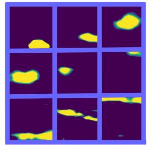
Figure 15 shows isocontours of the probability for different topics. One can see that some consist of streaks or ‘legs’ with a strong streamwise coherence near the wall (15a–c) while others consist of lumps farther away from the wall (15d–f), which may be reminiscent of ‘heads’ and are not always connected to the wall. It is unclear whether the lack of connection between ‘legs’ and ‘heads’ is an artefact of the limited domain size or whether this constitutes evidence of wall-detached coherent structures. An investigation over a larger domain will be necessary in order to settle this question.

Figure 15. Examples of 3-D topics represented by their isoprobability contour  $p=16$
  $10^{-5}$. The topics indexed with
  $N$ were selected out of a total number of topics
  ${N_T}=48$. The probability for each topic sums to unity over the domain. Here (a)
  $N=33$; (b)
  $N=38$; (c)
  $N=42$; (d)
  $N=46$; (e)
  $N=7$; (f)
  $N=16$.
The characteristic dimensions of the motifs are reported in figure 16. Since the number of samples is small, we checked that the trends reported below held for 2-D motifs identified on wall-parallel planes at different heights. Further,  $L_y$ appears to grow linearly over both regions. Two different regions can be identified based on the evolution of the horizontal dimensions. The critical height separating the two regions is of the order of
  $y_+ \sim 100$, in agreement with experimental observations (Stanislas, Perret & Foucaut Reference Stanislas, Perret and Foucaut2008). For
  $y_+ \lessapprox 100$ the region is characterized by a wide distribution of
  $L_x$ and
  $L_z$, with a ratio of
  $L_x/L_z$ that varies between 2 and 8. For
  $y_+ \gtrapprox 100$ both
  $L_x$ and
  $L_z$ appear to increase nearly linearly with a ratio that decreases slowly to a value of the order of 2 (with a standard deviation of 1). This ratio is consistent with results from analysis of POD eigenfunctions in Podvin et al. (Reference Podvin, Fraigneau, Jouanguy and Laval2010), as well as from vortex cluster analysis from Alamo et al. (Reference Alamo, Jimenez, Zandonade and Moser2006). Three-dimensional motif characteristic sizes are consistent with those obtained for vertical planes, which shows that information about the 3-D organization of the flow can be obtained from analysis performed on 2-D sections. This is of particular interest as it suggests that the LDA method could be usefully applied to particle image velocimetry experimental data limited to a plane. We also note that the data do not have to be resolved in time.

Figure 16. (a) Characteristic dimensions of the 3-D motifs,  ${N_T}=144$; the dashed line corresponds to the fit
  $y_+$ and the dotted line to a
  $4 y_+^{1/2}$ fit. (b) Evolution of ratio
  $L_x/L_z$ with height for
  $N_T=144$ and
  $N_T=48$. The dashed line corresponds to a mean value of 2.
6. Field reconstruction and generation
6.1. Reconstruction
We now examine how the flow can be reconstructed using LDA. In all that follows, without loss of generality, we will focus on one of the cross-flow planes examined in § 5, specifically the cross-section at  $x=0$ of dimensions
  $d_{y+}=590$ and
  $d_{z+}=450$. As described in the algorithm presented in § 3, both the motif–snapshot and the cell–motif distributions can be sampled for the total intensity
  $N_{i} = \sum _{l} f_{{l},{i}}$ in the
  ${i}$th snapshot. This total intensity is defined as the rescaled integral value of the Reynolds stress (digitized and restricted to
  $Q_-$ events) over the plane. Since results were found to be essentially independent of the rescaling, we can make the simplifying assumption that
  $N_{i}$ is large enough so that the distribution
  $\varphi _{{n}}$ is well approximated by the samples. For a given total intensity
  $N_{i}$, a reconstruction of the
  ${i}$th snapshot can then be obtained at each grid cell
  $\boldsymbol {x}_{l}$ from
 \begin{equation} \tau^{R\text{-}LDA}(\boldsymbol{x}, t_{i}) = \frac{1}{A} f_i(\boldsymbol{x}) = \frac{N_{i}}{A} \sum_{{n}=1}^{{N_T}} \theta_{{n}, {i}} \varphi_{{n}}(\boldsymbol{x}), \end{equation}
where
(i)
$\varphi _{{n}}(\boldsymbol {x})$ is the motif–cell distribution;(ii) the snapshot–motif distribution
$\theta _{{n}, {i}}$ represents the likelihood of motif $\boldsymbol {z}_{{n}}$ in the ${i}$th snapshot.


It seems natural to compare this reconstruction with the POD representation of the field which has a similar expression,
 \begin{equation} \tau^{R\text{-}POD}(\boldsymbol{x},t_{i})= \sum_{{n}=0}^{N_{POD}-1} a_{{n},{i}} \phi_{{n}}(\boldsymbol{x}), \end{equation}
where
(i)
$\phi _{{n}}(\boldsymbol {x})$ are the POD eigenfunctions extracted from the autocorrelation tensor $C_{{i}, {i}'}$ obtained from the ${{N_s}}$ snapshots;(ii)
$a_{{n},{i}}$ corresponds to the amplitude of the ${n}$th POD mode in the ${i}$th snapshot.


The first six fluctuating POD modes are represented in figure 17. We note that the zeroth POD mode represents the temporal average of the field. As expected, the fluctuating POD modes consist of Fourier modes in that spanwise direction (due to homogeneity of the statistics), and their intensity reaches a maximum at around  $y_+ \simeq 25$.

Figure 17. Contour plot of the first six fluctuating normalized POD spatial modes; contour values go from  $-0.03$ to
  $0.03$. Negative values are indicated by dashed lines.
  $(a)\ n = 1, \ (b)\ n = 2, \ (c)\ n = 3, \ (d)\ n = 4, (e)\ n = 5, \ (\,f)\ n = 6. $
If the number of POD modes is equal to the number of motifs  ${N_T}$, by construction, POD will provide a better representation of the statistics at least up to second order (Holmes et al. Reference Holmes, Lumley and Berkooz1996). We note that, in terms of computational requirement, POD is less expensive than LDA, as it requires solving an SVD problem versus implementing an iterative EM algorithm (Dempster et al. Reference Dempster, Laird and Rubin1977). However, the performance of the EM algorithm can be improved, in particular with online updates (Hofmann Reference Hofmann1999).
In terms of storage, a reconstructed snapshot requires  $N_{POD}$ modes for POD and
  ${N_T}$ topics for LDA. However, storage reduction could be obtained in the case of LDA by filtering out the motifs with a low probability
  $\theta _{{n}, {i}}$, i.e. lower than a threshold
  $\kappa$. We note that, in this case, it is necessary to store the indices
  ${n}$ of the motifs as well as the value of
  $\theta _{{n}, {i}}$, so that if
  $n$ modes (respectively, topics) are kept, storage will consist of
  $2 n$ variables per snapshot. We see that storage reduction can be achieved if the fraction of retained modes
  $\eta =n/{N_T}$ is sufficiently small. The LDA storage data length per snapshot
  $2 \eta {N_T}$ should then be compared with the POD data length
  $N_{POD}$.
For  ${N_T}=96$, choosing a threshold of
  $\kappa =0.015$ resulted in less than 8 % difference between the filtered and unfiltered LDA reconstructions (the
  $L_2$ norm was used). The average value for
  $\eta$ was
  $0.2$, which means that the number of POD modes that would represent a storage equivalent to that of LDA with
  ${N_T}=96$ is
  $N_{POD} \simeq 2 \eta {N_T} \simeq 40$. We note that the total storage cost should further take into account the size of the LDA basis
  $\{\boldsymbol {z}_{{n}}\}_{{n}}$, which will be larger than the POD basis
  $\{\boldsymbol {\phi }_{{n}}\}_{{n}}$ since they are, respectively, equivalent to
  ${N_T}$ and
  $N_{POD}$ fields. However, efficient storage of the LDA basis can be achieved by making use of the limited spatial support of
  $\boldsymbol {z}_{{n}}$, in particular for motifs located close to the wall.
In the remainder of this section we will compare a filtered LDA reconstruction of 96 motifs (where values of  $\theta _{{n}, {i}}$ lower than
  $\kappa =0.015$ are excluded from the reconstruction), with a POD representation of
  $N_{POD}=48$ modes, which captures approximately 75 % of the total energy. Figure 18 compares an instantaneous field with its LDA reconstruction and its POD reconstruction. A more general assessment is provided by figure 19, which shows the correlation coefficient between each snapshot and its reconstruction based on POD as well as that based on LDA. Although POD appears to be slightly superior, as can be expected from its optimality property, the correlation coefficients are very close with respective average values of 0.75 for LDA and 0.77 for POD.

Figure 18. Instantaneous Reynolds stress field (limited to  $Q_-$ events) (a) True field; (b) LDA-reconstructed field using 96 modes; (c) POD-reconstructed field using 48 modes.

Figure 19. Distribution of the correlation coefficient between each original snapshot and its reconstruction based on (a) LDA or (b) POD.
6.2. Generation
Latent Dirichlet allocation is a generative model, so it is straightforward to generate synthetic snapshots by sampling from distributions  $\theta$ and
  $\varphi$ for a total intensity
  $N_{{i}}=\sum _{{l}} f_{{l}, {i}}$, which is modelled as a Poisson process with the same mean and standard deviation as the original database.
In contrast, POD is not a generative model per se. We will use a simplified version of the probabilistic extension of POD (PPCA) derived by Tipping & Bishop (Reference Tipping and Bishop1999), which is presented in Appendix B, where we will make the additional assumption that no noise is present in the model, POD-based synthetic fields will be reconstructed from deterministic spatial POD modes  $\boldsymbol {\phi }_{{n}}$ and random POD amplitudes
  $\boldsymbol {a}_{{n}}$ which are assumed to be Gaussian variables. Examination of figure 20, which represents the distribution of the first fluctuating POD coefficients
  ${n} \ge 1$, suggests that it is quite acceptable as a first approximation to assume Gaussian distributions for the amplitudes
  $\boldsymbol {a}_{{n}}$ – alternatively, the amplitudes could be sampled from the empirical distributions. The amplitude of the zeroth mode, which corresponds to the average of the field over the snapshots, will be assumed to be constant for all snapshots.

Figure 20. Histograms of the normalized amplitudes of the first six fluctuating POD modes and comparison with a sampled Gaussian distribution.  $(a)\ n = 1, \ (b)\ n = 2, \ (c)\ n = 3, \ (d)\ n = 4, \ (e)\ n = 5, \ (\,f)\ n = 6.$
We can therefore compare the databases reconstructed from and generated with LDA with those obtained from POD. The generated databases consist of  ${{N_s}}$ snapshots corresponding to arbitrary instants
  $\tilde {t}_{i}$. Overall, the statistics of five different databases can be compared:
(i) the true database
$\tau _-(y,z,t_{i})$ corresponding to the actual values of the $Q_-$ events;(ii) the POD-reconstructed (R-POD) or POD-projected database,
(6.3)where\begin{equation} \tau_-^{R\text{-}POD}(y,z,t_{i}) = \sum_{{n}=0}^{N_{POD}-1} a_{{i},{n}} \phi_{{n}}(y,z), \end{equation}$\phi _{{n}}$ are the POD eigenfunctions and $a_{{i},{n}}$ are the amplitudes of the ${n}$th POD mode in the ${i}$th snapshot;(iii) the POD-generated (G-POD) database,
(6.4)where\begin{equation} \tau_-^{G\text{-}POD}(y,z,\tilde{t}_{i}) = \sum_{{n}=0}^{N_{POD}-1} \tilde{a}_{{i},{n}} \phi_{{n}}(y,z), \end{equation}$\tilde {a}_{{i},0}=\langle a _{{i},0}\rangle$, with $\langle \cdot \rangle$ the average over all snapshots and $\tilde {a}_{{i},{n}}$, ${n} \geq 1$, centred Gaussian random variables with variance $\langle \tilde {a}_{{i},{n}}^2\rangle$;(iv) the LDA-reconstructed database (R-LDA),
(6.5)where\begin{equation} \tau_-^{R\text{-}LDA}(y,z,t_{i}) = \frac{N_{i}}{A} \sum_{{n}=1}^{{N_T}} \theta_{{n}, {i}} \varphi_{{n}}(y,z), \end{equation}$N_{i}$ is the total intensity measured in the ${i}$th snapshot, $\theta _{{n}, {i}}$ is the distribution of motif ${n}$ on the ${i}$th snapshot and $\varphi _{{n}}(y,z)$ is the identified distribution of the cell at $(y,z)$ on motif ${n}$.(v) the LDA-generated database (G-LDA),
(6.6)where\begin{equation} \tau_-^{G\text{-}LDA}(y,z,\tilde{t}_{i}) = \frac{\tilde{N}_{i}}{A} \sum_{{n}=1}^{{N_T}} \tilde{\theta}_{{n},{i}} \varphi_{{n}}(y,z), \end{equation}$\tilde {N}_{i}$ is the total intensity, which is sampled from a Poisson process, $\varphi _{{n}}(y,z)$ is the identified distribution of the cell at $(y,z)$ on motif ${n}$ and $\tilde {\theta }_{{n},{i}}$ is sampled for each ${n}$ from the empirical distribution $\theta _{{n}, {i}}$ over the snapshots.


Figure 21 shows the statistics of the different databases as a function of the wall distance. Averages are taken over all snapshots and in the streamwise direction. The mean value of the Reynolds stresses is correctly recovered by all methods. The second-order statistics are slightly better recovered by the POD-reconstructed and POD-generated snapshot sets, but both LDA approaches also capture a significant portion of the variance. The POD databases capture 75 % of the total variance, while the reconstructed and generated LDA databases capture 68 % and 60 % of the variance, respectively. Again, the superiority of POD over LDA is expected since it is optimal in the L2 sense, however, it should be noted that the gain is relatively small. Figure 22 shows the vertical spatial autocorrelation of  $\tau _-$ defined as
  $R(y, y')=\langle \tau _-(x,y,z,t)\tau _(x,y',z,t)\rangle$ (where
  $\langle \cdot \rangle$ represents an average taken in time and in the spanwise position). We can see that the generated LDA autocorrelation is very similar to its reconstructed POD counterpart, which shows that the LDA synthetic fields capture as much as the spatial structure as the POD reconstructed ones. We note that the autocorrelation at large separations is well reproduced by all datasets.

Figure 21. Statistics of the different databases averaged over the spanwise direction and the number of snapshots: (a) mean value; (b) standard deviation.

Figure 22. Spatial autocorrelation of the Reynolds stress (limited to  $Q_-$ events) in the vertical direction at different heights. The average is taken over snapshots and in the spanwise direction.
  $(a)\ y_{0+} = 33, (b)\ y_{0+} = 163.$
Figure 23 shows histograms of the fields at different heights. We note that unlike the LDA approach, which is a non-negative decomposition (since it is based on probabilities), some negative values are observed for the POD approach, even though the original field values considered are always positive. We can see that at different wall distances the POD-reconstructed database reproduces well the distribution of the original database, but the POD-generated database does not. This failure is due to the fact that although POD amplitudes are uncorrelated by construction, they are not independent. We note that the same failure was observed when sampling the POD coefficients from their data-observed distributions  $a_{{i}, {n}}$ instead of Gaussian processes. In contrast, both reconstructed and generated LDA methods yield very similar distributions, which reproduce the main features of the original Reynolds stress values, such as the intermittency (sharp peak at zero) and the asymptotic decay for positive values. The LDA is therefore able to reproduce strongly non-Gaussian statistics, which is not possible with its POD equivalent.

Figure 23. Histograms of the Reynolds stress (limited to  $Q_-$ events) corresponding to the different databases at different heights.
  $(a,\!b)\ y_{+} = 19, \ (c,\!d)\ y_{+} = 61, \ (e,\!f)\ y_{+} = 157, \ (g,\!h)\ y_{+} = 343.$
7. Conclusion
This paper presents exploratory work about the application of LDA to the identification of coherent structures in turbulent flows. In the probabilistic framework of LDA, latent factors or motifs are inferred from a collection of snapshots. Each snapshot is characterized by a motif distribution, and each motif itself is distributed over space. Implementation was carried out for a scalar field representing Reynolds stress  $Q_-$ events. Evidence of self-similarity was found in the motifs: the spanwise and vertical dimensions of the motifs increase linearly with the wall distance in the logarithmic region, and the number of structures evolves inversely with the wall distance. This is in agreement with the eddy attached model hypotheses. The characteristics of the motifs were established to be robust with respect to the LDA parameters.
Latent Dirichlet allocation yields a sparse, efficient reconstruction of the snapshots that compares reasonably well with POD representation. Adding in the fact that the motifs have a local spatial support, even when statistics are homogeneous, could make the LDA representation of interest for estimation and control purposes. Further, a strong benefit of LDA is its inherent generative property, which makes it possible to generate a set of synthetic snapshots which is statistically similar to the original one. In particular, strongly non-Gaussian features are captured and can be reproduced by the LDA representation.
The first results obtained with the LDA method open up exciting prospects for data analysis and modelling of turbulent flows. The present study was carried out at a moderate Reynolds number for domains which are relatively small compared with the typical extent of coherent structures. The observations will therefore need to be confirmed in larger domains at higher Reynolds numbers in future work.
In addition, while the investigation was limited to a positive scalar field in the present implementation, it would be useful to extend the capabilities of LDA to fully real, as well as multidimensional fields. One possibility to handle real fields would be to code the field sign into the cell index, which would be equivalent to considering two different, positive scalar fields on two identical grids.
Moreover, the LDA technique appears well suited to describe intermittent phenomena, since it decomposes the domain of investigation into a set of localized regions (motifs), each of which is characterized by a specific, snapshot-dependent intensity. It would, therefore, be interesting to apply it to strongly inhomogeneous flow regions such as the turbulent/non-turbulent interface (Philip et al. Reference Philip, Meneveau, de Silva and Marusic2014) or other types of intermittency (Johnson & Meneveau Reference Johnson and Meneveau2017).
Acknowledgements
The authors are grateful to the anonymous Referees for their helpful comments on the first version of the manuscript.
Funding
This work was supported by the Center of Data Science from the Paris-Saclay University. Computations were carried out at IDRIS-GENCI (project 02262).
Declaration of interests
The authors report no conflict of interest.
Appendix A. LDA as a factorization method
To further shed light on the interpretation of LDA, we now adopt a different viewpoint and briefly explore the connections between the decomposition methods discussed above in the framework of MF. Specifically, we now explain how model decomposition methods, such as POD, k-means and LDA, can be interpreted in terms of MF.
A.1. MF
Letting  ${F}\in \mathbb {R}^{{N_x}\times {{N_s}}}$ be a data matrix to be approximated, MF consists in the following decomposition:
 \begin{equation} {F} = X Y, \end{equation}
with  $X\in \mathbb {R}^{{N_x}\times {N_T}}$ and
  $Y\in \mathbb {R}^{{N_T}\times {{N_s}}}$ two real-valued matrices. Compression is achieved whenever
  ${N_T} <\min ({N_x},{{N_s}})$, which is considered hereafter. Matrix factorization can be formulated as an optimization problem,
with  $\left \|{\cdot }\right \|_{}$ a given norm,
  $\mathcal {S}_X$ and
  $\mathcal {S}_Y$ admissibility sets for
  $X$ and
  $Y$, respectively, and
  $\mathcal {R}$ a regularization term.
A.2. POD–MF equivalence
Let the SVD of the  ${N_x} \times {{N_s}}$ real-valued data matrix
  ${F}$ be
 \begin{equation} {F} = \varPsi \varSigma B^{\mathrm{T}}, \end{equation}
with  $\varPsi$ and
  $B$ two orthonormal matrices and
  $\varSigma$ being diagonal. The Eckart–Young theorem makes precise in which sense this decomposition is optimal (Eckart & Young Reference Eckart and Young1936). In particular, it follows that
where  $(\varSigma B^{\mathrm {T}})_{N_T} = \varSigma _{N_T} B_{N_T}^{\mathrm {T}}$ and with
  $\varPsi _{N_T}$ and
  $B_{N_T}$ the restriction of
  $\varPsi$ and
  $B$ to their columns associated with the dominant
  ${N_T}$ singular values
  $\mathrm {diag}(\varSigma _{N_T})$.
From (A3), it follows that
 \begin{equation} {F} {F}^{\mathrm{T}} \varPsi = \varPsi_{N_T} \varSigma_{N_T} B_{N_T}^{\mathrm{T}} B_{N_T} \varSigma_{N_T}^{\mathrm{T}} \varPsi_{N_T}^{\mathrm{T}} \varPsi_{N_T} = \varPsi_{N_T} \varSigma_{N_T}^2 = C_{N_T} \varPsi_{N_T}. \end{equation}
 Referring to (2.1) and (2.2), the diagonal matrix  $\varSigma _{N_T}^2$ and
  $\varPsi _{N_T}$ then directly identify with the
  ${N_T}$ dominant eigenvalues
  $\varLambda$ and POD modes
  $\varPhi$, respectively. Denoting the Moore–Penrose pseudo-inverse with a
  $+$ superscript, the POD projection coefficients are
 \begin{equation} A = \varPhi^+ {F} = \varPhi^{\mathrm{T}} {F} = \varPsi_{N_T}^{\mathrm{T}} {F} = \varSigma_{N_T} B_{N_T}^{\mathrm{T}}, \end{equation}
so that the POD decomposition is finally seen to satisfy the following MF problem:
of the form of (A2) with  $\mathcal {R} \equiv 0$ and
  $\mathcal {S}_X$ such that
  $X^{\mathrm {T}} X = I_{N_T}$.
A.3. k-means–MF equivalence
Clustering is an unsupervised learning technique aiming at identifying groups (clusters) in the data such that data points in the same group have similar features, while data points in different groups have highly dissimilar features.
One of the simplest and popular clustering methods is k-means (MacQueen Reference MacQueen1967; Lloyd Reference Lloyd1982). The algorithm tries to iteratively partition the dataset into  ${N_T}$ predefined distinct non-overlapping clusters
  $\{ \mathcal {C}_{{n}} \}_{{n}}$. In its standard deterministic version, each data point belongs to only one cluster. The key idea consists in assigning each data point to the closest centroid (arithmetic mean of all the data points that belong to that cluster). The distance is defined in terms of some chosen norm
  $\left \|{\cdot }\right \|_{}$. Setting the number of clusters
  ${N_T}$, the algorithm starts with an initial guess for the
  ${N_T}$ centroids
  $\{ \boldsymbol {c}_{{n}} \}_{{n}}$, by randomly selecting
  ${N_T}$ data points from the data set without replacement. It then iterates between the data assignment step, assigning each data point
  ${f}_{{i}}$ to the closest cluster
  $\mathcal {C}_{{n}_{i}^\star }$ and the centroid update step, which computes the centroid of each cluster,
 \begin{gather}\boldsymbol{c}_{{n}} \gets \frac{1}{\mathrm{card}\left[\mathcal{C}_{{n}}\right]} \sum_{{f}_{{i}} \in \mathcal{C}_{{n}}} {f}_{{i}}, \quad \forall \ 1 \le {n} \le {N_T}. \end{gather}
 Furthermore, k-means is guaranteed to converge to a local optimum but not necessarily to a global optimum. Therefore, we choose to run the algorithm with different initializations of centroids and retain the solution that yielded the lowest loss  $\mathscr {L}$,
 \begin{equation} \mathscr{L} = \sum_{{n}=1}^{N_T} {\sum_{{f}_{i} \in \mathcal{C}_{{n}}}{\left\|{{f}_{i} - \boldsymbol{c}_{{n}}}\right\|_{}^2}}. \end{equation}
 Solving a clustering problem in the  $L^2$ sense means finding a set of
  $\{\mathcal {C}_{{n}}\}_{{n}=1}^{N_T}$ disjoint clusters (
 $\mathcal {C}_{{n}} {\bigcap} \mathcal {C}_{{n}^{'}} =\{\emptyset \}$,
  ${n} \ne {n}^{'}$), that minimizes the following cost function:
 \begin{equation} \mathscr{L} = \sum_{{n}=1}^{N_T} {\sum_{{f}_{i} \in \mathcal{C}_{{n}}}{\left\|{{f}_{i} - \boldsymbol{c}_{{n}}}\right\|_{2}^2}} = \sum_{{i}=1}^{{N_s}} {\left\|{{f}_{i}}\right\|_{2}^2} - \sum_{{n}=1}^{N_T} {\sum_{{f}_{i}, {f}_{{i}'} \in \mathcal{C}_{{n}}}{ n_{{n}}^{{-}1} {f}_{i}^{\mathrm{T}} {f}_{{i}'} }}, \end{equation}
where  $\{\boldsymbol {c}_{{n}}\}_{{n}=1}^{N_T}$ are the cluster centroids,
  $\boldsymbol {c}_{{n}} := \sum _{{f}_{i} \in \mathcal {C}_{{n}}} {{f}_{i}} / n_{{n}}$,
  $n_{{n}} := \mathrm {card}\left [\mathcal {C}_{{n}}\right ]$.
Let  $Y\in [0,1]^{{{N_s}} \times {N_T}}$ be the normalized cluster indicator matrix,
 ![]() . Disjointedness of clusters implies that columns of
. Disjointedness of clusters implies that columns of  $Y$ are orthonormal,
  $Y^{\mathrm {T}} Y= I_{N_T}$. The clustering problem (A11) may now be reformulated in terms of
  $Y \ge 0$ as (Ding, He & Simon Reference Ding, He and Simon2005)

The Euclidean hard-clustering k-means problem hence stems from an orthogonal non-negative matrix factorization form and the clusters are given by  $\boldsymbol {c}_{{n}} = n_{{n}}^{-1/2} {F} \boldsymbol {y}_{{n}}$,
  $\forall {n}$.
A.4. LDA–MF equivalence
We now focus on LDA and discuss the fact that, similarly to POD and k-means, it can also be interpreted as a MF technique, under certain conditions.
Let us consider the variational LDA flavour, where inferring the LDA parameters from maximizing the posterior distribution  $p$ is substituted with an approximated posterior
  $q$, easier to sample from. The inference problem then consists in minimizing the approximation error, which is equivalent to maximizing the evidence lower bound (ELBO)
  $\mathscr {L}$,
 \begin{equation} \mathscr{L} = \mathbb{E}_{\mu_q}\left[p\right] - \mathbb{E}_{\mu_q}\left[q\right]. \end{equation}
 Provided suitable approximations in the inference problem are made, and under a symmetric Dirichlet priors hypothesis  $(\boldsymbol {\alpha } = \alpha \boldsymbol {1})$, Faleiros & Lopes (Reference Faleiros and Lopes2016) have derived an upper bound for the ELBO associated with variational LDA,
 \begin{equation} \max \mathscr{L} \lessapprox \min \sum_{{l}}^{N_x} { \sum_{i}^{{N_s}}{\left({F}_{{l}, {i}}\log {\frac{{F}_{{l}, {i}}}{{\left(X Y\right)}_{{l}, {i}}}} + \sum_{{n}}^{N_T}{\mathcal{R}(Y_{{n},{i}}, \alpha_{{n}})}\right) }}, \end{equation}
where  $X \geq 0$ and
  $Y \geq 0$ are variational parameters to be inferred, normalized as
  $\sum _{{l}}X_{{l}, {n}}=\sum _{{n}}Y_{{n}, {i}}=1$, and regarded as normalized probability distributions. Here,
  $\boldsymbol {x}_{{n}}$ is related to
  ${\boldsymbol {\beta }}$ while
  $\boldsymbol {y}_{i}$ is related to the distribution
  $\boldsymbol {\theta }_{i}$ of a document
  ${f}_{i}$. The term
  $\mathcal {R}(Y_{{n}, {i}},{\alpha }_{{n}}) := (Y_{{n}, {i}} - {\alpha }_{{n}})(\log Y_{{n}, {i}} - Y_{{n}, {i}}(\log Y_{{n}, {i}}-1))$ corresponds to the prior influence and induces sparsity over the document-topic distribution.
From (A14), it follows that maximizing the ELBO  $\mathscr {L}$ under certain approximations takes the form of a non-negative MF problem (known as NMF) of
  ${F} \approx X Y$ expressed in terms of the Kullback–Leibler divergence,
 \begin{equation} D_{I}({F}\|X Y) := \sum_{{l}, {i}}{ \left({F}_{{l}, {i}}\log {\frac{{F}_{{l}, {i}}}{{(X Y)}_{{l}, {i}}}}-{F}_{{l}, {i}}+{(X Y)}_{{l}, {i}} \right)}, \end{equation}
supplemented with a regularization term.
Details of the derivation are beyond the scope of this paper and one should refer to Faleiros & Lopes (Reference Faleiros and Lopes2016) for a more complete discussion.
Appendix B. PPCA/POD
In this section, we give a brief review of PPCA (Tipping & Bishop Reference Tipping and Bishop1999) which provides a density estimation framework for POD (or PCA/LSA), under hypotheses that are different from those given in § 2.2 for PLSA.
We will assume that the data is zero-centred, without loss of generality. The basic idea of PPCA is to assume a Gaussian probability model for the observed data  $f'$. In that formulation (see § 2.2), the motif–cell matrix
  $\tilde {\varPhi }$ of dimension
  $N_x \times {N_T}$ does not have a probabilistic interpretation, but relates each noisy observation to a set of
  ${N_T}$ independent normalized Gaussian variables following
 \begin{equation} f' = \tilde{\varPhi} \tilde{a} + \epsilon, \end{equation}
where the variables  $\tilde {a}$ are defined to be independent and Gaussian with unit variance and
  $\epsilon$ represents noise.
An important assumption to proceed is that the model for the noise should be isotropic,
 \begin{equation} \langle \epsilon \epsilon \rangle = \sigma^2 I, \end{equation}
so that all the dependences between the observations are going to be contained in  $\tilde {\varPhi }$. One can then show using (B1) that
 \begin{equation} p(f') = {\mathcal{N}}(0, C ), \end{equation}
where  $C= \tilde {\varPhi }^T \tilde {\varPhi } + {\sigma }^2 I$ is the observation covariance matrix of dimension
  $N_x^2$.
The issue is to determine  $\tilde {\varPhi }$ and
  $\tilde {\sigma }$, given the observations of
  $f'$. Under the assumption of isotropic Gaussian noise, Tipping & Bishop (Reference Tipping and Bishop1999) showed that the maximum likelihood estimators
  $\hat {\varPhi }$ and
  $\hat {\sigma }^2$ can be obtained from standard POD analysis on the
  ${{N_s}}$ snapshots. They showed that
 \begin{equation} \hat{\varPhi}= \varPhi ( \varLambda_{nmode} - \sigma^2 I_{{N_T}})^{1/2} R, \end{equation}
where  $\varPhi$ contains the first
  ${N_T}$ eigenvectors of the sampled covariance matrix
  $\tilde {C}$ where
  $\tilde {C}$ was defined in (2.4) (note that the dimension of
  $\tilde {C}$ is
  ${{N_s}}^2$),
  $\varLambda _{{N_T}}$ is a diagonal matrix containing the
  ${N_T}$ first eigenvalues of
  $\tilde {C}$ and
  $R$ is an arbitrary rotation matrix.
An estimate for the error variance can then be given by
 \begin{equation} \hat{\sigma}^2 = \frac{1}{{{N_s}} - {N_T} }\sum_{j={N_T} + 1}^{{{N_s}}} \lambda_j, \end{equation}
which represents the variance lost in the project and averaged over the lost dimensions.


