
Weed seeds in the soil (i.e., the weed seedbank) are the primary source of weed infestations in most crop fields (Cavers and Benoit Reference Cavers and Benoit1989; Gallandt Reference Gallandt2006). Both empirical and modeling studies indicate that managing the weed seedbank is key to successful long-term management of annual agricultural weeds (Davis Reference Davis2006; Davis et al. Reference Davis, Cardina, Forcella, Johnson, Kegode, Lindquist, Luschei, Renner, Sprague and Williams2005). Practices that target the weed seedbank are particularly important for organic cropping systems, where weed control options are limited due to prohibitions against most types of herbicides (Teasdale et al. Reference Teasdale, Mangum, Radhakrishnan and Cavigelli2004). Consequently, much research has been conducted in a variety of organic and conventional cropping systems to understand how specific agronomic management practices such as tillage, herbicide use, cover cropping, and crop rotation impact weed seedbanks (e.g., Moonen and Barberi Reference Moonen and Barberi2004; Sosnoskie et al. Reference Sosnoskie, Herms and Cardina2006; Squire et al. Reference Squire, Rodger and Wright2000).
Despite recognizing the importance of the weed seedbank to the success of overall weed management, we know surprisingly little about how factors that are not under direct control of farmers, such as weather and site-specific edaphic factors either individually or in combination, affect the composition and species abundance of weed seedbanks (Pakeman et al. Reference Pakeman, Small and Torvell2012; Peters et al. Reference Peters, Breitsameter and Gerowitt2014). This information could contribute to the development of more effective weed management strategies for both organic and conventionally managed cropping systems. For instance, some edaphic factors, such as soil pH, organic matter content, and concentrations of some macro- and micronutrients, strongly influence the activity of soil microbial communities and are amenable to modification through agronomic management. If some of these edaphic factors are found to be strongly linked with weed seed survival and persistence, then altering these could serve as alternative weed management strategies (Kremer and Li Reference Kremer and Li2003).
Such information is also critical for better understanding and modeling the effects of climate change on agriculture (Wortman et al. Reference Wortman, Davis, Schutte, Lindquist, Cardina, Felix, Sprague, Dille, Ramirez, Reicks and Clay2012), particularly at regional scales. If climatic rather than edaphic factors are the primary determinants of weed seedbank composition and abundance on farm fields, then climate change models could be used to predict weed species range expansions and contractions, enabling farmers to better prepare for changes in the weed communities they manage (Chen et al. Reference Chen, Hill, Ohlemuller, Roy and Thomas2011; Peters et al. Reference Peters, Breitsameter and Gerowitt2014).
Results from previous research attempting to link the composition or dynamics of weed seedbanks to abiotic factors have been mixed. Schwartz et al. (Reference Schwartz, Gibson, Gage, Matthews, Jordan, Owen, Shaw, Weller, Wilson and Young2015) examined weed seedbank composition and diversity across 150 conventionally row-cropped sites spanning six states in relation to geo-climatic (hardiness zone, latitude, and longitude), edaphic (soil texture), and management factors. Out of 16 species they analyzed, 10 were associated with distinct U.S. Department of Agriculture (USDA) hardiness zones. Hardiness zone was also strongly related to weed seedbank composition, total seedbank density, and species richness and diversity, while management variables (e.g., crop rotation, frequency of glyphosate-resistant crops), in contrast, were not strongly related to seedbank communities. These results matched patterns in the emergent weed communities that were also measured at each site (Young et al. Reference Young, Gibson, Gage, Matthews, Jordan, Owen, Shaw, Weller and Wilson2013). Similarly, in a seedbank augmentation study conducted across 8 states, Davis et al. (Reference Davis, Cardina, Forcella, Johnson, Kegode, Lindquist, Luschei, Renner, Sprague and Williams2005) found that seed persistence in 8 of 15 annual weed species was negatively related to hydrothermal time (which integrates soil matric potential and temperature); however, the strength of the relationship depended on weed species and never accounted for more than 35% of the variation. The authors attributed some of this remaining variation to the influence of edaphic variables, including bulk density, soil texture, and organic carbon (Davis et al. Reference Davis, Cardina, Forcella, Johnson, Kegode, Lindquist, Luschei, Renner, Sprague and Williams2005). While both studies are suggestive of strong geo-climatic controls on seedbank species composition and the demographic parameters that regulate internal weed seedbank dynamics, each also encompassed large geographic ranges that could potentially confound climatic, edaphic, and other sources of variation, including herbicide application. Additionally, studies that span large geographic ranges are more likely to include disparate geographic species pools, potentially confounding climatic and edaphic limitations to weed community membership with limitations occurring due to dispersal constraints (sensu Belyea and Lancaster [Reference Belyea and Lancaster1999] and Kelt et al. [Reference Kelt, Taper and Meserve1995]).
In contrast to these regional studies, research conducted at local scales, where weather and climate conditions do not vary and geographic species pools are similar or are under researcher control, have found that edaphic factors can be important determinants of weed seed persistence in soils. For example, Pakeman et al. (Reference Pakeman, Small and Torvell2012) found that across 12 semi-natural and grassland sites located within 3.5 km, seed survival in 12 plant species was strongly dependent on the characteristics of the soil. Specifically, ungerminated seeds survived longer in soils with a higher pH, low moisture content, and lower soil C:N. Other studies conducted across small spatial scales have similarly found soil characteristics to be strong determinants of seed persistence (Long et al. Reference Long, Steadman, Panetta and Adkins2009; Narwal et al. Reference Narwal, Sindel and Jessop2008) and emergent weed community composition (Andreasen et al. Reference Andreasen, Streibig and Haas1991). Thus, taken together, previous work conducted across large spatial scales suggests that geo-climatic factors are the dominant drivers of weed seedbanks, while work conducted at small spatial scales suggests that edaphic factors dominate. Surprisingly, however, there have been few studies that have attempted to determine the relative importance of geo-climatic versus edaphic factors across relatively small spatial scales where both of these types of factors vary but where geographic species pools are expected to be similar.
Northern New England (NNE) encompasses a relatively small spatial area (the states of Maine, New Hampshire, and Vermont) but relatively high variability in both climate and soils (Keim and Rock Reference Keim and Rock2001). This high variability is due, in part, to the region’s proximity to the Atlantic Ocean, which moderates temperature extremes in the coastal portions of Maine and New Hampshire, and the elevation gradients created by the White and Green mountain chains of the Appalachians that run through large portions of New Hampshire and Vermont, respectively, and the Longfellow Mountains in Maine. For example, the 220 km that separate East Charleston, VT, from Portsmouth, NH, encompasses six USDA plant hardiness zones (3b to 6a). Few areas of the United States span such a range in climate across a comparatively small spatial extent. Interestingly, a 2012 update to the USDA Plant Hardiness Zone Map (USDA PHZM) based on more recent temperature records (USDA 2012) and recent changes to the Canadian hardiness zone map resulted in northward shifts in most zones, reflecting contemporary climate warming (McKenney et al. Reference McKenney, Pedlar, Lawrence, Papadopol, Campbell and Hutchinson2014). Simulation studies indicate that dramatic shifts in these zones are likely to continue in the future (Parker and Abatzoglou Reference Parker and Abatzoglou2016). The NNE region is therefore ideal for studying climate change impacts on weed communities, because it encompasses a large degree of climate and edaphic variation across a relatively small spatial area and therefore may serve as a harbinger of future climate change impacts in other regions.
The primary objective of this study was to assess the relative importance of climate-related versus edaphic factors in determining weed seedbank community composition and abundance on organic farms across the NNE region. We hypothesized that at the regional-level, weed seedbank communities would exhibit a strong climate “signal” due to the wide variation in climate across the region, and hence geo-climatic variables would be stronger correlates with weed seedbank communities relative to edaphic variables. An additional objective was to assess the degree to which weed communities could be differentiated based on the USDA plant hardiness zone in which each farm was located. Hardiness zones range from 3b (average annual extreme minimum temperature −37.2 to −34.4 C) to 6a (−23.3 to −20.6 C) across the three-state region (USDA 2012). We hypothesized that hardiness zones effectively integrate multiple geographic and climatic variables (such as elevation or proximity to unfrozen water bodies), and therefore weed communities would be strongly differentiated across these zones. Finally, we hypothesized that at smaller scales of analysis (i.e., state level), edaphic variables would emerge as stronger correlates with weed seedbanks, particularly in states that encompass narrower ranges in hardiness zones.
Materials and Methods
Weed Seedbank Sampling and Greenhouse Assay
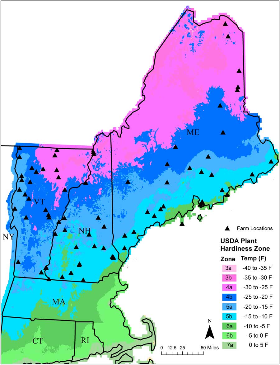
We collected soil samples in spring of 2013 from 77 organic farms across NNE (Figure 1). The majority of these farms grew vegetables, while a few grew small grains. Farms in the region tend to be small and diversified and are often separated from other farms by extensive tracts of forests and woodland (Hale et al. Reference Hale, Wollheim, Smith, Asbjornsen, Brito, Broders, Grandy and Rowe2014). Farms chosen for sampling were intended to provide broad geographic coverage across each of the three states. At each farm, we chose a single field for seedbank sampling. The field chosen for sampling had been tilled and/or cultivated the previous season and was identified by the farmer as being especially “weedy.” To sample the seedbank in each field, we collected three sets of five soil cores (total of 15 soil cores) across the field to a depth of 10 cm using a 7.6-cm-diameter bulb planter (Yard Butler IBPL-6 Bulb and Garden Planter, Lewis Tools, Poway, CA). Each set of five soil cores was bulked and placed in an individually labeled bag that was then placed in a cooler for transport back to the university greenhouse facility in its respective state. Two of the bulked samples from each farm (each containing five soil cores) were used for a germination assay aimed at quantifying the readily germinable fraction of the weed seedbank. The third set of soil cores was sent to the University of Maine Soil Testing Service for soil chemical and physical analysis (described in the following section).

Figure 1 USDA Plant Hardiness Zone Map showing approximate locations of the 77 organic farms (black triangles) that were sampled in Maine, New Hampshire, and Vermont.
The two bulked soil samples used for the germination assay were spread evenly on trays filled with soilless growing medium (medium-coarse vermiculite) and placed in a climate-controlled greenhouse facility. Soil trays were watered as necessary to maintain moist (but not saturated) soil conditions. Trays were monitored regularly, and weed seedlings that emerged from the trays were identified and removed with forceps. Any seedlings that could not be identified were transplanted into pots and grown until identification was possible. This process continued until seedling emergence slowed and then stopped for a period of a week. At that point, soils in all trays were allowed to dry completely. Soils were then broken up and stirred, and the trays were then rewatered to stimulate additional weed seedling emergence. This process was repeated over the course of 6 mo. Weed seedling values for the two bulked soil samples were averaged to obtain mean species composition and abundance estimates for each site.
Edaphic, Geographic, and Climatic Data
Soil samples collected at each of the 77 farms were sent to the University of Maine Soil Testing Service in Orono, ME. The analysis included soil textural (percent sand, silt, and clay), biological (soil carbon, measured as loss on ignition), and chemical measurements (pH and concentrations of calcium [Ca], potassium [K], magnesium [Mg], phosphorus [P], aluminum [Al], boron [B], copper [Cu], iron [Fe], manganese [Mn], sodium [Na], sulfur [S], and zinc [Zn]), as well as effective cation exchange capacity (ECEC). In addition to the soil physical and chemical data, we also acquired geographic and climatic data specific to each farm sampled. The geographic data included the latitude, longitude, and elevation of each farm, and the climatic data included select weather variables. The climatic data were acquired from the Weather Underground (www.wunderground.com). In all cases we chose data from the weather station located closest to the farm and for the time period of the year prior to sampling (January to December 2012). In some cases, the same weather station was used for multiple farms. The weather data included: cumulative growing degree days (base of 10 C; hereafter SumGDD); average daily maximum (MeanMaxTemp), mean (MeanTemp), and minimum (MeanMinTemp) temperature; absolute minimum temperature (MinTemp); and total precipitation (Precip.). We chose to restrict the weather data to the year preceding seedbank sampling with the rationale that the majority of seeds present in the readily germinable fraction of the seedbank in spring would have come from weeds that were present the previous summer and fall (Smith and Gross Reference Smith and Gross2006).
We also used the revised USDA PHZM (USDA 2012) to determine the zone in which each farm was located. The hardiness zone represents the mean extreme minimum temperature, calculated from the lowest daily minimum temperature recorded at a site, using weather data from 1976 to 2005 (USDA 2012). Alphabetical subzones within zones (e.g., 5a and 5b) were converted to quantitative variables (e.g., 5.0 and 5.5, respectively) prior to analysis. Ranges and means for the edaphic and geo-climatic variables associated with the soil samples and corresponding sampling locations within each state are presented in Table 1.
Table 1 Ranges (minimum and maximum) and means for geo-climatic and edaphic variables associated with soils sampled at farms in each of the three states.
a Abbreviations: ECEC, effective cation exchange capacity; LOI, soil carbon; MeanMaxTemp, average daily maximum temperature; MeanMinTemp, minimum temperature; MeanTemp, mean temperature; MinTemp, absolute minimum temperature; SumGDD, cumulative growing degree days (base 10 C).
Data Analysis
Prior to conducting statistical analyses, we calculated several variables that summarized the weed seedbank community at each of the 77 farms. Total weed seedling density was calculated by summing all individuals of all species that emerged from the soil sample. We calculated several indices of seedbank diversity, each emphasizing different aspects of community structure. These indices included species richness (the sum of all species represented within a sample), Shannon diversity, H′=−Σp i 2 (log p i ), where p i is the proportion of seedlings accounted for by species i per sample (Magurran Reference Magurran1988); evenness, E=H′/ln (species richness); and Simpson’s index of diversity, D=1−Σp i 2 (McCune and Grace Reference McCune and Grace2002).
The weed seedbank community composition, abundance, and community summary data, soil chemical and physical variables, and geographic and weather variables were then analyzed at two spatial scales using multivariate procedures. The primary objectives of these analyses were to characterize variation in weed seedbank community composition and abundance at both the regional and individual state scales and to relate this variation in community structure to geographic, weather, soil variables, and USDA plant hardiness zone. Our ultimate aim was to determine the relative importance of geo-climatic versus edaphic factors in driving variation in weed seedbank community composition and abundance at both the regional and state scales.
Regional-Scale Analyses
Nonmetric multidimensional scaling (NMDS) ordination (McCune and Grace Reference McCune and Grace2002) was used to characterize the variation in the weed seedbank community across the farms. In addition to enabling us to visualize patterns in community variation associated with the weed seedbanks at each farm, this approach allowed us to reduce the weed community data set to two or three synthetic variables (i.e., NMDS ordination axis scores) that captured the majority of the variation in the original distance matrix. These synthetic variables were then used as response variables in subsequent analyses (described below). Prior to performing NMDS, species occurring in fewer than 5% of the farms were omitted from the data set to reduce the influence of extremely rare species. All remaining species abundance values were log(x+1) transformed. A dissimilarity matrix using Bray-Curtis coefficients was then calculated from the transformed species abundance values. Two hundred and fifty runs of the ordination (at random starting configurations and with a maximum of 500 iterations per run) were performed with an instability criterion of 0.0000001. The runs were compared with 250 randomized runs to assess the significance of the reduction in stress from six to one dimensions (Monte Carlo test).
Following NMDS, we used Pearson (parametric) and Kendall (nonparametric) correlations to assess the strength and directionality of relationships between the NMDS axes, representing the variation in weed seedbank communities across the farms, and the individual soil, geo-climatic, and weed community summary variables.
To assess whether differences in weed communities associated with plant hardiness zones were statistically significant, we used multiresponse permutation procedures (MRPP; McCune and Grace Reference McCune and Grace2002) using the same dissimilarity coefficient matrix (Bray-Curtis) used for the NMDS. MRPP is a nonparametric, permutation-based test for differences between or among groups of sample units (in this case weed communities on individual farms grouped by plant hardiness zone) based on within-group similarities in composition and abundance (Peck Reference Peck2010).
In cases in which MRPP indicated that weed communities differed based on hardiness zone, we used indicator species analysis (ISA; Dufrene and Legendre Reference Dufrene and Legendre1997) to determine which species were associated with specific hardiness zones. Indicator values (IV) for each weed species were calculated by multiplying the relative abundance and relative frequency of each weed species in each hardiness zone. For each species, the significance of the highest IV, which corresponds to the hardiness zone with which it was most associated, was tested with a Monte Carlo procedure (1,000 permutations) at the P≤0.05 level.
The NMDS ordinations, correlation analyses, MRPP, and ISA were conducted in PC-ORD v. 6.08 (McCune and Mefford 2011; MjM Software, Gleneden Beach, OR).
To assess the relative importance of geo-climatic versus edaphic factors in driving weed seedbank community variation across the region we used nonparametric multiplicative regression (NPMR; McCune Reference McCune2006). We chose a nonparametric regression model because we anticipated that weed community responses to weather and edaphic variables would be complex, interactive, and nonlinear. The approach is qualitatively different from traditional modeling tools in that NPMR does not seek a fixed mathematical equation, but rather relies on the data to determine model form using a local multiplicative smoothing function with a leave-one-out cross-validation (Miller et al. Reference Miller, Wooster and Li2007). All analyses were conducted using a local mean estimator and Gaussian weighting function in forward stepwise regressions. We assessed model fit with a cross-validated R2 (xR2), as this is more conservative than traditional R2, because each data point is excluded from calculating the residual sums of squares for the response at that point. We developed individual NPMR models for each of the NMDS ordination axis scores and weed community summary variables (i.e., total seedling density, species richness, and the three diversity indices). For all analyses, we chose the best (highest xR2) one- to four-predictor variable models using a significance level of P<0.05. Sensitivity analysis was used to assess the relative influence of individual explanatory variables within each selected model (McCune Reference McCune2006). Sensitivities were generated by changing values of individual predictor variables to measure the resulting change in the response variable at that point. For example, a sensitivity value of 1.0 would indicate equal change in the response variable per unit change in the predictor across their respective ranges; a sensitivity of 0 would indicate that a change in the predictor has no effect on the response variable. Additional details regarding NPMR theory, implementation, and interpretation are provided by McCune (Reference McCune2006) and Miller et al. (Reference Miller, Wooster and Li2007). All NPMR analyses were conducted in HyperNiche v. 2.3 (McCune and Mefford Reference McCune and Mefford2009; MjM Software, Gleneden Beach, OR).
State-Level Analyses
To examine finer-scale (i.e., state-level) variation in weed seedbank communities, variation that could be obscured by strong geographic gradients in the regional analysis, we created individual weed community matrices for each state. For each state-level data matrix, we omitted species occurring in fewer than 5% of the farms sampled (i.e., rare species) and then log(x+1) transformed the data. We then conducted NMDS, correlation, and MRPP analyses in the manner described for the regional analyses.
To examine the relative importance of geo-climatic versus edaphic factors at the state level, we used partial least-squares regression (PLSR). PLSR is a multivariate technique that uses latent variables (factors) to determine the relationship between predictor and response variables and has advantages over traditional multiple regression approaches, as well as NPMR, in that it performs well when sample sizes are low relative to the number of predictors or when predictors are highly correlated (Carrascal et al. Reference Carrascal, Galvan and Gordo2009). Wortman et al. (Reference Wortman, Davis, Schutte, Lindquist, Cardina, Felix, Sprague, Dille, Ramirez, Reicks and Clay2012) used PLSR to analyze the relative importance of environmental factors on the demography of several weed species, and they provide additional background on the approach. For our analysis we constructed separate PLSR models for the individual weed community response variables for each state. The response variables were the individual NMDS ordination axis scores and the weed community summary variables (i.e., total seedling density, species richness, and the three diversity indices). Predictor variables with variable importance values greater than 0.8 were retained in the final models. We used the approach of Carrascal et al. (Reference Carrascal, Galvan and Gordo2009) to determine the number of factors (i.e., components) to retain in each model (i.e., those explaining more than 5% of the variance in the response variable). Model predictive ability was determined with K-fold cross-validation, with K=7. All PLSR analyses were conducted using the NIPALS algorithm in JMP Pro software v. 12.1 (SAS Institute, Cary, NC).
Results and Discussion
Regional Analysis
We identified a total of 113 weed species in seedbank samples collected across the 77 farms. The eight most abundant weed species, in terms of total number of seedlings that emerged from the seedbank samples, were from highest to lowest: slender rush (Juncus tenuis Willd.), hairy galinsoga (Galinsoga quadriradiata Cav.), common purslane (Portulaca oleracea L.), Veronica spp., common lambsquarters (Chenopodium album L.), redroot pigweed (Amaranthus retroflexus L.), large crabgrass [Digitaria sanguinalis (L.) Scop.], and low cudweed (Gnaphalium uliginosum L.); together these accounted for nearly 73% of the total seedlings that emerged from the samples. No species were present in all 77 sites; however, nine species occurred in at least 65% of the sites. These nine species were common lambsquarters (observed in 95% of the farms), large crabgrass (82%), redroot pigweed (78%), hairy galinsoga (70%), slender rush (68%), common chickweed [Stellaria media (L.) Vill.] (68%), Veronica spp. (68%), yellow woodsorrel (Oxalis stricta L.) (66%), and broadleaf plantain (Plantago major L.) (65%).
Not unexpectedly, there was also variation in weed seed density and diversity across the 77 farms that we sampled. Weed seedling density (a proxy for germinable weed seed density) ranged from 1,119 to 53,471 m−2 (mean=15,151 m−2) across the 77 sites. Species richness and evenness ranged from 5 to 31 (mean=18.8) and 0.15 to 0.84 (mean=0.62), respectively. Shannon’s and Simpson’s indices of diversity ranged from 0.40 to 2.61 (mean=1.77) and 0.13 to 0.89 (mean=0.72), respectively.
Relationships between the Weed Seedbank Communities and Geo-climatic and Edaphic Variables
The NMDS ordination of the regional weed seedbank data set resulted in a three-dimensional solution that accounted for a total of 80% of the variation in the original distance matrix (NMDS, stress=16.6, P=0.004). Pearson correlations between the NMDS axes and weed community summary variables (Table 2) indicated that NMDS axis 1, which accounted for 45.4% of the variation in the weed seedbank community, was associated with variation in both total weed species richness (R2=0.48) and weed seedling density (R2=0.24).
Table 2 Pearson (r and R2) and Kendall (tau) correlations with nonmetric multidimensional scaling (NMDS) axes from the regional data set of weed seedbank communities from farms sampled in Maine, New Hampshire, and Vermont.Footnote a

a Bolded values indicate strong (R2 > 0.2) Pearson correlations.
b Abbreviations: ECEC, effective cation exchange capacity; HardZone, USDA plant hardiness zone; MeanMaxTemp, average daily maximum temperature; MeanMinTemp, minimum temperature; MeanTemp, mean temperature; MinTemp, absolute minimum temperature; SumGDD, cumulative growing degree days (base 10 C).
Pearson correlations between the NMDS axes and the geo-climatic and edaphic variables (Table 2) indicated that variation in weed seedbank community composition and abundance across the 77 farms was correlated with both types of variables. However, among the variables having relatively strong (R2>0.2) Pearson correlations with either NMDS axis 1 or 2, the strongest correlates tended to be geo-climatic variables. The strongest geo-climatic correlate with NMDS axis 1 was longitude (R2=0.61). Other strong correlates were SumGDD (R2=0.27) and MeanMaxTemp (R2=0.26). The second NMDS axis, which accounted for 20.3% of the variation in the weed seedbank community, was strongly correlated only with latitude (R2=0.27). Latitude and longitude, along with elevation, were also identified as strong correlates with the emergent weed floras sampled across 80 agricultural fields in Alaska; however, the authors ascribed these relationships to differences in the types of crops and associated weed control practices occurring at higher and lower latitudes and longitudes (Conn et al. Reference Conn, Werdin-Pfisterer and Beattie2011). In our study these confounding factors are less likely because our focus was on seedbanks, all of our farms were organic, and all but a few of the farms grew vegetable crops. Latitude and longitude were both negatively correlated with growing degree days and maximum temperatures (data not shown), suggesting that at least some of the apparent correlation due to geographic position reflects variation in temperature along the latitudinal and longitudinal gradients (see also Nowak et al. Reference Nowak, Nowak, Nobis and Nobis2015). Similarly, Fried et al. (Reference Fried, Norton and Reboud2008) analyzed emerged weed communities in 700 arable fields across France and observed that latitudinal and longitudinal gradients, reflecting variation in both temperature and precipitation, explained substantial variation in species composition.
In contrast to the geo-climatic variables, none of the edaphic variables had Pearson correlations stronger than R2=0.26 with any of the NMDS axes (Table 2). Edaphic variables with relatively strong (R2 > 0.2) Pearson correlations with NMDS axis 1 were soil pH (R2=0.26), Al (R2=0.24), and Mn (R2=0.23). No edaphic variables were strong correlates with NMDS axis 2. The third NMDS axis, which accounted for 13.7% of the remaining weed seedbank community variation, was not strongly correlated with any of the geo-climatic or edaphic variables. The correlation between soil pH and seedbank composition is congruent with some previous research (Andreasen et al. Reference Andreasen, Streibig and Haas1991; Fried et al. Reference Fried, Norton and Reboud2008; Pakeman et al. Reference Pakeman, Small and Torvell2012; but see Nowak et al. Reference Nowak, Nowak, Nobis and Nobis2015). The mechanisms underlying possible seedbank regulation by soil pH are unclear, but could include toxicity from aluminum or other heavy metals, or changes in the fungal:bacterial ratio of the soil microbial community that affect seed decay (Pakeman et al. Reference Pakeman, Small and Torvell2012). Soil pH can also affect the quantity of seed inputs to the soil by affecting growth and subsequent seed production in some weed species (Wada et al. Reference Wada, Altland, Mallory-Smith and Stang2006).
Simple correlations between the geo-climatic and edaphic variables and the NMDS axes may mask more complex interactions or nonlinearities among the geo-climatic and edaphic variables and the weed seedbank communities. To account for these types of interactions and assess relationships between these variables and weed density and diversity, we constructed NPMR models for each weed community response variable (i.e., the three NMDS axes, weed diversity indices, weed species richness, and total weed seedling density). In general, these models confirmed the importance of the geo-climatic variables, either alone or in combination with edaphic variables, in predicting weed community composition and abundance across the region (Table 3). The most parsimonious models for each of the first two NMDS ordination axes were both two-predictor models that explained 74% and 51% of the variation in the NMDS axis 1 and axis 2 scores, respectively. Longitude was the variable with the highest model sensitivity in both models, highlighting its importance as a predictor of weed community composition. The model for NMDS axis 1 also included MeanTemp, while MeanMaxTemp was included in the model for NMDS axis 2. Longitude and precipitation, along with soil carbon (%LOI), were also the most sensitive variables in the most parsimonious model describing total weed density (Table 3). Longitude was also included in the model for species richness; however, it was less sensitive compared with the two edaphic variables also included in the model (sodium and percent clay). The model for Simpson’s index of diversity, which identified soil pH and SumGDD as the most explanatory variables, was the only significant model that did not include longitude as a predictor variable. The two- and three-predictor NPMR models for Shannon diversity, while only slightly above our threshold for statistical significance, had relatively low explanatory power (xR2=0.17, P=0.07 and xR2=0.22, P=0.06, respectively). NPMR models for NMDS axis 3 and species evenness were not significant (P>0.1). In general, these results are congruent with previous work showing, at regional scales, that the environmental factors that drive variation in emergent weed community composition are not necessarily the same as those that drive variation in weed species diversity (Fried et al. Reference Fried, Norton and Reboud2008).
Table 3 Nonparametric multiplicative regression model results for germinable weed seedbank community parameters generated from the regional data set of farms sampled in Maine, New Hampshire, and Vermont.Footnote a , Footnote b

a Abbreviations: %LOI, soil carbon determined by loss on ignition; MeanTemp, mean temperature; MeanMaxTemp, mean daily maximum temperature; NMDS, nonmetric multidimensional scaling; Precip., precipitation; SumGDD, cumulative growing degree days (base 10 C).
b Bolded models are those in which model P<0.05 and inclusion of additional predictor variables does not increase xR2>5%.
c Sensitivities reflect the relative importance of the geo-climatic and edaphic predictor variables; a value of 1 indicates a proportionally equal change in the response variable per unit change in the predictor variable, while a value of 0 would indicate that a change in the predictor variable has no effect on the response variable.
Associations between Plant Hardiness Zones and Weed Communities
The NMDS ordination of the weed seedbank community indicated apparent groupings of weed communities based on both plant hardiness zone and state political boundary (Figure 2). We used MRPP to determine whether weed communities differed based on the hardiness zone in which the farm was located. Weed seedbank community groups based on plant hardiness zones (Figure 2A) were significantly different (MRPP, A=0.04, P<0.0001). Based on ISA, weed species associated with hardiness zone 3 were barnyardgrass [Echinochloa crus-galli (L.) Beauv.] (ISA, IV=51.6, P=0.04), scentless chamomile [Tripleurospermum perforata (Mérat) M. Lainz ] (IV=42.0, P=0.02), knawel (Scleranthus annuus L.) (IV=39.3, P=0.03), and common groundsel (Senecio vulgaris L.) (IV=35.2, P=0.05). Only one species was associated with hardiness zone 4 (common lambsquarters, IV=32.8, P=0.05), while no species were associated with hardiness zone 5. Only fringed willowherb (Epilobium ciliatum Raf.) was associated with hardiness zone 6 (IV=52.5, P<0.01).
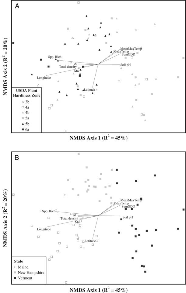
Figure 2 Nonmetric multidimensional scaling (NMDS) ordination of germinable weed seedbank communities sampled on 77 organic farms across Maine, New Hampshire, and Vermont. Seedbank communities are coded by USDA plant hardiness zone (A) or state political boundary (B). Joint plots indicate Pearson correlations (R2 ≥ 0.2) between ordination axis scores and geo-climatic, edaphic, and weed community summary variables. MeanMaxTemp, average daily maximum temperature; MeanTemp, mean temperature; Spp. Rich, species richness; SumGDD, cumulative growing degree days (base 10 C).
Relatively few farms were located in hardiness zones 3 and 6 relative to the other two zones (4 and 5); therefore, we also analyzed species associations with just hardiness zones 4 and 5. When farms located in zones 3 and 6 were omitted from the analysis, four species were associated (ISA, P<0.05) with hardiness zone 4, [in order of decreasing IV: common lambsquarters, orchardgrass (Dactylis glomerata L.), birdsrape mustard (Brassica rapa L.), and ladysthumb (Polygonum persicaria L.)], and three were associated with hardiness zone 5 [in order of decreasing IV: slender rush, Veronica spp., and carpetweed (Mollugo verticillata L.)]. These results are qualitatively similar to those observed by Schwartz et al. (Reference Schwartz, Gibson, Gage, Matthews, Jordan, Owen, Shaw, Weller, Wilson and Young2015) and Young et al. (Reference Young, Gibson, Gage, Matthews, Jordan, Owen, Shaw, Weller and Wilson2013) for weed seedbank and emergent weed communities, respectively, sampled across the conventional row-crop growing regions of the central and southern United States.
While the grouping of weed communities based on plant hardiness zone was significant, MRPP indicated that an even stronger grouping of weed communities was based on state political boundaries (MRPP, A=0.15, P<0.0001; Figure 2B). This result is somewhat curious, and could reflect strong east–west gradients in temperature or other geo-climatic factors across the three states. Another explanation, however, could be slight differences in how the seedbanks were sampled by investigators in each state or the growing conditions specific to the greenhouses in which each state’s germination assays were conducted. While the three states followed identical protocols for both sampling and the germination assay, we cannot entirely discount these as potential contributors to the patterns we observed in the regional data set. Such sources of experimental error would not be present in the state-level analyses.
State-Level Analyses
Given that our regional analysis has the potential to obscure more subtle but potentially important patterns of association between seedbank community composition and geo-climatic and edaphic variables, we also analyzed the weed seedbanks associated with each state separately. These state-level analyses also provided a means of assessing the relative consistency of individual correlates with weed communities across the three states.
Within-State Gradients
The Maine data set included 30 farms and encompassed the largest gradients in geo-climatic variables among the three states. For example, the farms sampled in Maine spanned latitudinal and longitudinal gradients of 43.3°N to 47.2°N and 70.68°W to 67.15°W, respectively, and an elevation gradient from sea level to 238 m. Consequently, the farms ranged in plant hardiness zones from 3b to 6a (Figure 1). In contrast, the farms sampled in New Hampshire (22) and Vermont (25) spanned relatively shorter gradients in both latitude (NH: 42.73°N to 44.97°N; VT: 42.84°N to 44.98°N) and longitude (NH: 72.52°W to 70.94°W; VT: 73.34°W to 72.15°W), but larger gradients in elevation (NH: 25.6 to 520.3 m; VT: 33.8 to 381.9 m). The range in hardiness zones was also smaller in New Hampshire (zones 3b to 5b) and Vermont (zones 4a to 5a) compared with Maine.
Relationships between the Weed Seedbank Communities and Geo-climatic and Edaphic Variables
NMDS ordination of the weed seedbanks sampled from the farms in Maine resulted in a three-dimensional solution that accounted for 79.5% of the variation in the original distance matrix (NMDS: stress=15.53, P=0.004). The first NMDS axis accounted for the majority of the variation (R2=43.5%) and had strong (R2>0.2) Pearson correlations with five of the geo-climatic variables. The strongest geo-climatic correlate was latitude (R2=0.48), followed by hardiness zone (0.42), MeanMinTemp (0.29), elevation (0.23), and MinTemp (0.23). In contrast, only four edaphic variables were strong correlates, and none of the correlations exceeded R2=0.30. The strongest edaphic correlates were percent sand (R2=0.30), percent silt (0.25), magnesium (0.25), and copper (0.22). The second NMDS axis accounted for an additional 24.3% of the variation and was strongly correlated only with MeanMaxTemp (R2=0.25). The third NMDS axis, which accounted for 11.7% of the variation, was not strongly correlated with any of the geo-climatic or edaphic variables. These results are congruent with the analysis of the regional data set, in that geographic position and temperature variables tended to be the stronger correlates with seedbank composition.
Analyses of the New Hampshire and Vermont data sets yielded results similar to those of the Maine data set, in that there were more strong geo-climatic than edaphic correlates with the seedbanks in each state. NMDS ordination of the weed seedbanks sampled from the farms in New Hampshire resulted in a three-dimensional solution that accounted for 76.7% of the variation in the original distance matrix (NMDS: stress=13.98, P=0.012). Variation was relatively evenly distributed across NMDS axes 1 through 3 (R2=25.2%, 27.6%, and 24.0%, respectively). Elevation, MeanMaxTemp, hardiness zone, and latitude all had Pearson correlations (R2) ranging from 0.22 to 0.28. Hardiness zone was strongly correlated with both NMDS axes 1 and 3, while the other three geo-climatic variables were each correlated with only one of the NMDS axes. In contrast, the only edaphic variables with strong Pearson correlations were iron (R2=0.33 with NMDS axis 1) and percent clay (R2=0.20 with NMDS axis 3).
The ordination of the weed seedbanks sampled from the farms in Vermont resulted in a two-dimensional solution that accounted for 63.5% of the variation in the original distance matrix (NMDS: stress=23.07, P=0.028). NMDS axes 1 and 2 accounted for 36% and 27.5% of the variation, respectively. Among the geo-climatic variables, precipitation was the only variable strongly correlated with the first NMDS axis (R2=0.20). MinTemp (R2=0.27), MeanTemp (R2=0.24), and SumGDD (R2=0.21) were strong correlates with the second axis. None of the edaphic variables were strong correlates with either of the axes. The fact that hardiness zone was not a strong correlate in the Vermont data set may have been due to the relatively narrow range of zones sampled in Vermont compared with those sampled in New Hampshire and Maine (Table 1; Figure 1).
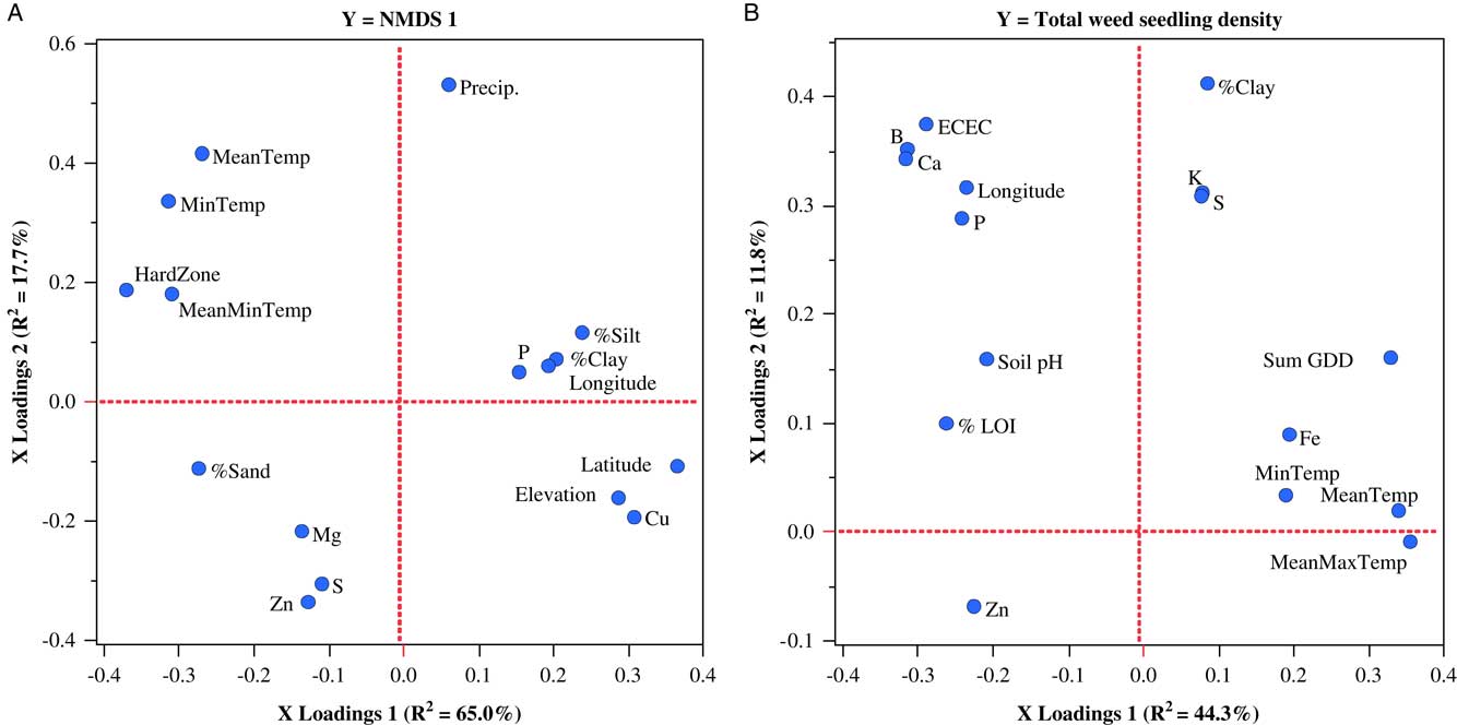
Similar to the regional analysis, we also used regression models to examine how the combination of geo-climatic and edaphic variables might have contributed to the variation in weed seedbank communities measured in each state and to identify the most important variables associated with that variation. In this case, we used PLSR, due to its ability to perform well when sample size is small and the number of predictor variables is large (Carrascal et al. Reference Carrascal, Galvan and Gordo2009). In general, results of the individual PLSR models of the weed seedbank communities sampled in each state reinforced the importance of the geo-climatic variables in explaining community variation. In fact, all of the models, with the exception of the model explaining Shannon diversity of the weed seedbank in the Vermont samples, were more heavily influenced by geo-climatic than edaphic variables. A two-factor PLSR model containing 16 predictor variables explained a total of 83% of the variation in the first axis of the NMDS conducted on the Maine data set. Variables loading most strongly on PLSR factor 1 were hardiness zone (negative loading) and latitude (positive loading), while those loading most strongly on PLSR factor 2 were precipitation (positive loading) and zinc (negative loading) (Figure 3A). Models for NMDS axes 2 and 3 contained no minimizing number of factors (P>0.05) and therefore were not explanatory. The only other weed community variable from the Maine data set that could be modeled with PLSR was total weed seedling density. Variables with strong positive loadings with the first PLSR factor, which accounted for 44.3% of the variation in weed density, were MeanMaxTemp, MeanTemp, and SumGDD, while variables with the strongest negative loadings were boron, calcium, ECEC, and soil carbon (LOI) (Figure 3B). This result is congruent with research demonstrating that weed growth and weed seed production, and hence inputs to the soil seedbank, are often positively associated with warmer temperature conditions (e.g., Hyvönen Reference Hyvönen2011), and the role that soil organic matter and associated soil conditions may play in regulating weed seed decay by soil microorganisms (Fennimore and Jackson Reference Fennimore and Jackson2003; Liebman and Davis Reference Liebman and Davis2000).

Figure 3 Factor-loading scatter plots for partial least-squares regression (PLSR) models for nonmetric multidimensional scaling (NMDS) axis 1 (A) and total weed seedling density (B) of germinable weed seedbank communities sampled on 30 organic farms in Maine. %LOI, soil carbon; ECEC, effective cation exchange capacity; HardZone, USDA plant hardiness zone; MeanMaxTemp, average daily maximum temperature; MeanMinTemp, minimum temperature; MeanTemp, mean temperature; MinTemp, absolute minimum temperature; Precip., total precipitation; SumGDD, cumulative growing degree days (base 10 C).
Weed seedbank communities sampled in New Hampshire could be accounted for by separate two-factor PLSR models that explained 52.2% and 63.8% of the variation in NMDS axes 1 and 3, respectively. Variables loading most strongly on the first factor of the model for NMDS axis 1 included latitude, elevation, SumGDD, and MeanTemp (Figure 4A), while variables loading most strongly on the first factor of the model for NMDS axis 3 were MeanTemp, hardiness zone, SumGDD, MinTemp, and latitude (Figure 4B). There were no significant models for NMDS axis 2 or any of the weed community summary variables.
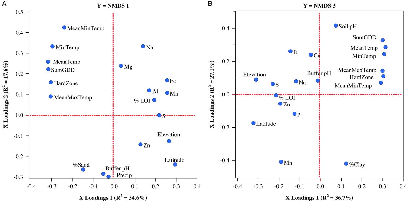
Figure 4 Factor-loading scatter plots for PLSR models for NMDS axis 1 (A) and NMDS axis 3 (B) characterizing germinable weed seedbank communities sampled on 22 organic farms in New Hampshire. %LOI, soil carbon; ECEC, effective cation exchange capacity; HardZone, USDA plant hardiness zone; MeanMaxTemp, average daily maximum temperature; MeanMinTemp, minimum temperature; MeanTemp, mean temperature; MinTemp, absolute minimum temperature; Precip., total precipitation; SumGDD, cumulative growing degree days (base 10 C).
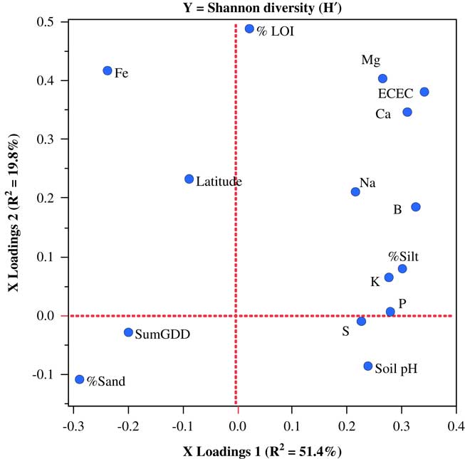
Only one weed seedbank community variable from the Vermont data set, Shannon diversity, could be modeled with PLSR. In this case, a two-factor PLSR model explained 71.2% of the variation in seedbank diversity. In contrast to the models for weed community parameters in the other two states, variables loading most strongly on PLSR factor 1 were almost entirely edaphic (Figure 5).

Figure 5 Factor-loading scatter plots for partial least-squares regression (PLSR) models for the Shannon diversity of germinable weed seedbanks sampled on 25 organic farms in Vermont. %LOI, soil carbon; ECEC, effective cation exchange capacity; SumGDD, cumulative growing degree days (base 10 C).
Associations between Plant Hardiness Zones and Weed Communities
Weed seedbank communities sampled on farms in Maine and Vermont could be differentiated by plant hardiness zone, but only when subzones a and b were combined within each numerical zone (Maine: MRPP, A=0.034, P=0.03; Vermont: MRPP: A=0.023, P=0.01). Differentiation among the weed communities based on zone was also visually apparent in the NMDS ordinations (Figure 6). In contrast, weed seedbank communities in New Hampshire did not differ between plant hardiness zones (MRPP: A=0.01, P=0.16). Within the Maine data set, four weed species were significant indicators of hardiness zone 4 (common lambsquarters, IV=42.2, P=0.001; orchardgrass, IV=44.4, P=0.013; Trifolium spp., IV=46.0, P=0.043; and narrowleaf groundsel [Euthamia graminifolia (L.) Nutt.], IV=40.3, P=0.029), none were indicators of zone 5, and three were indicators of zone 6 (yellow woodsorrel, IV=55.1, P=0.005; fringed willowherb, IV=43.5, P=0.019; and ground ivy (Glechoma hederacea L.), IV=40.0, P=0.028). Weed species that were significant indicators of zone 4 in Vermont were smooth crabgrass [Digitaria ischaemum (Schreb.) Schreb. ex Muhl.] (IV=51.3, P=0.05) and yellow woodsorrel (IV=51.3, P=0.05). Species that were indicators of zone 5 in Vermont were lacegrass [Eragrostis capillaris (L.) Nees] (IV=55.0, P=0.006) and carpetweed (IV=43.7, P=0.021).
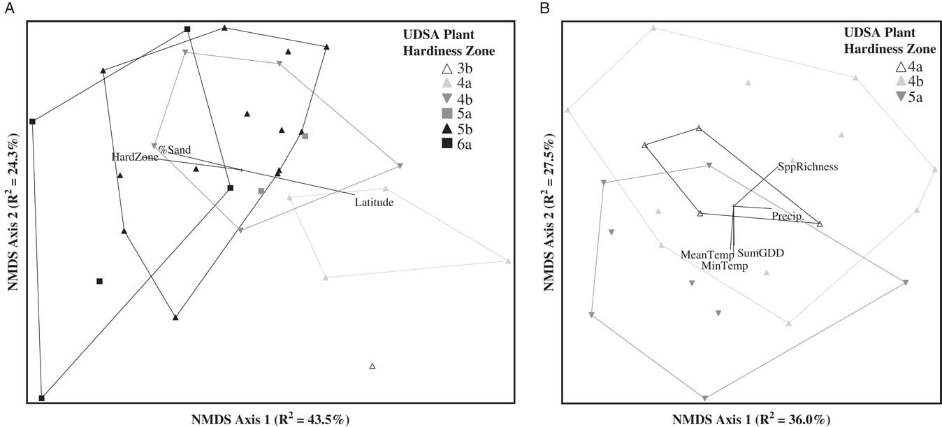
Figure 6 Nonmetric multidimensional scaling (NMDS) ordination of the germinable weed seedbank community sampled in Maine (A) and Vermont (B). Sample units coded by hardiness zone. Joint plots indicate Pearson correlations (R2 ≥ 0.2) between ordination axis scores and geo-climatic, edaphic, and weed community summary variables. HardZone, USDA plant hardiness zone; MeanTemp, mean temperature; MinTemp, absolute minimum temperature; Precip., total precipitation; SppRichness, species richness; SumGDD, cumulative growing degree days (base 10 C).
Comparing the regional and state-level ISA results indicates that there was little consistency between the specific weed species that were found to be associated with particular hardiness zones. This finding was somewhat unexpected but could indicate that populations of some of these species are locally adapted and therefore have evolved different climate optima or tolerances to other environmental factors compared with more distant populations, as has been observed in some weed species (e.g., Marcel et al. Reference Marcel, Lawson, Mortimer, Smilauerova, Bischoff, Cremieux, Dolezal, Edwards, Lanta, Bezemer, van der Putten, Igual, Rodriguez-Barrueco, Muller-Scharer and Steinger2007; Peters et al. Reference Peters, Breitsameter and Gerowitt2014). Only common lambsquarters was consistently associated with hardiness zone 4 in both the regional- and state-level (Maine) analyses. This too was somewhat surprising, given the relatively cosmopolitan distribution of this species.
Together, these analyses indicate a strong climate “signal” in the weed seedbank communities on organic farms in the NNE region. In general, temperature-related variables (latitude, longitude, mean maximum and minimum temperature), and to a lesser extent precipitation, appear to be the strongest and most consistent correlates with weed seedbank composition and abundance. This finding is particularly relevant to NNE, where growing seasons are expected to become warmer, wetter, and more variable (Fernandez et al. Reference Fernandez, Schmitt, Birkel, Stancioff, Pershing, Kelley, Runge, Jacobson and Mayewski2015). Edaphic variables were, for the most part, relatively weaker and inconsistent correlates with weed seedbanks. Our hypothesis that plant hardiness zones serve as useful proxies for the climatic conditions that regulate weed seedbank communities was generally supported, particularly at the state level of analysis. Our analyses suggest that a number of agriculturally important weed species are associated with particular hardiness zones, implying that future geographic shifts in climatic factors that delineate these zones (driven by climate warming) will likely lead to changes in the composition of weed communities and therefore new management challenges for farmers. These species, and in particular common lambsquarters, due to its consistent association with hardiness zone 4, may therefore warrant additional research with regard to their genetic potential for adaptation and expansion (Peters et al. Reference Peters, Breitsameter and Gerowitt2014). Our hypothesis that edaphic variables would emerge as stronger correlates with weed seedbanks at finer spatial scales of analysis was not well supported. In fact, there was only one case (species diversity on farms sampled in Vermont) in which edaphic variables were more strongly associated with seedbank variation compared with the geo-climatic variables. This suggests that improvements in the ability of climate models to predict future weed species occurrence, abundance, and distributions will likely arise from additional research aimed at better linking these parameters to climate and weather factors (e.g., Jarnevich et al. Reference Jarnevich, Holcombe, Barnett, Stohlgren and Kartesz2010) and that inclusion of edaphic variables into these models may provide only limited benefit. Our study did not consider other variables, such as CO2, that are also associated with climate change and can affect weed communities (e.g., Ziska Reference Ziska2003). Our study also did not consider the influence of specific agronomic and cropping practices (e.g., crop types and management practices), which would likely also change across the region in response to climate warming. Future research on weed–climate associations will therefore need to more fully link arable weed seedbank composition and abundance to climate and other environmental and agronomic factors that influence agricultural production systems and their associated weed communities.
Acknowledgments
We would like to thank the 77 farmers who allowed us to visit their farms and sample their soils. Technical assistance was provided by Liz Hodgdon, Kelsey Juntwait, Matt Morris, Samantha Werner, Nate Suhadolnik, David Goudreault, Jonathan Ebba, Brandan Crocker, and Hanna Renado. Avinash Rude helped generate the map that makes up Figure 1. Funding for this research was provided by the Northern New England Collaborative Research Funding Program. Partial funding was provided by the New Hampshire Agricultural Experiment Station. This is Scientific Contribution Number 2695. This work was supported by the USDA National Institute of Food and Agriculture Hatch Project 1006827.