The interpretation of cross-level direct effects in theoretical and research multilevel models

Although this issue has been discussed previously in the literature (LoPilato & Vandenberg, Reference LoPilato, Vandenberg, Lance and Vandenberg2015; see also Preacher, Zyphur, & Zhang, Reference Preacher, Zyphur and Zhang2010), it continues to be a source of misunderstanding. For illustrative purposes, suppose that the imaginary researcher we introduced in the first paragraph estimates the individual-level relationship between employee job burnout and employee well-being in each of the work teams making up his/her sample^{Footnote 2}. [Remember that s/he does so based on the idea that this relationship may vary across work teams depending on a team characteristic (support climate)]. Thus, s/he estimates a simple regression model in each team: Y = a + b X + e, where Y is the outcome variable (well-being), X is the predictor variable (job burnout), a is the regression intercept, b is the regression coefficient or slope, and e is the residual term. Using a multilevel notation and taking into account the nested structure of the data, the estimated regression model can be expressed as follows:

(1)$${Y_{ij}} = {\beta _{0j}} + {\beta _{1j}} \cdot {X_{ij}} + {r_{ij}}$$

where Y _ij is the score on the outcome variable of subject i from team j, X _ij is the score on the predictor variable of subject i from team j, β_0j is the regression intercept estimated in each team (j), β_1j is the regression coefficient (slope) estimated in each team (j), and r _ij is the residual term of the regression equation in each team (j). Note that in this equation the outcome and the predictor variables are individual-level variables (in the example case, job burnout and well-being, respectively). Thus, equation 1 is an individual-level equation.

Suppose that our researcher represents the regression lines obtained in each team in his/her sample and obtains a graph similar to the one represented in Figure 1 (in which, for the sake of clarity, only the regression lines of five teams are displayed).

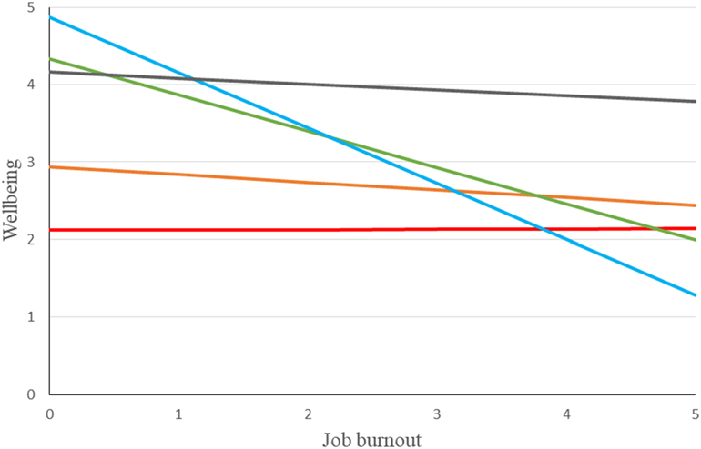
Figure 1. Regression lines obtained after regressing well-being at work on job burnout in five work teams.

Figure 1 points out that different teams show quite different regression lines. This means that there are differences across teams in the regression intercept (β_0j, the point at which the regression lines cross the Y-axis) and the regression slope (β_1j). In fact, the regression intercept varies between 2.1 and 4.9, and the slope between –.72 and 0. Because our researcher is interested in examining the sources of these variabilities in the regression intercepts and slopes across the j teams of his/her sample, and based on his/her idea that this variance may depend on work teams’ support climate (C_j), s/he writes the following simple regression equations of the Y = a + b X + e form:

(2)$${\beta _{0j}} = {\gamma _{00}}{\gamma _{01}} \cdot {C_j} + {U_{0j}}$$

(3)$${\beta _{1j}} = {\gamma _{10}}{\gamma _{11}} \cdot {C_j} + {U_{1j}}$$

Note that in these equations, the outcome variables (β_0j and β_1j) are two team characteristics (teams’ intercepts and slopes, respectively), and the predictor variable is also a team characteristic (support climate, C_j). Thus, equations 2 and 3 are team-level equations. Moreover, for the goals of this section, suffice it to say that γ₀₀ and γ₁₀ are two regression intercepts, γ₀₁ and γ₁₁ are two regression coefficients (slopes) that estimate the relationship between Cj, on the one hand, and β_0j and β_1j, on the other, and U _0j and U _1j are the corresponding residual terms.

Equations 1, 2, and 3 form a multilevel model in which different relationships are specified at different levels of analysis (the individual level: Equation 1, and the team level: Equations 2 and 3). Frequently, the terms β_0j and β_1j in Equation 1 are replaced with the corresponding right-hand parts of Equations 2 and 3, respectively. After some simple algebra and a rearrangement of terms, the following combined equation is obtained:

(4)$${Y_{ij}} = {\gamma _{00}} + {\gamma _{01}} \cdot {C_j} + {\gamma _{10}} \cdot {X_{ij}} + {\gamma _{11}}({C_j}{X_{ij}}) + ({U_{0j}} + {U_{1j}} \cdot {X_{ij}} + {r_{ij}})$$

The regression coefficient γ₀₁ is said to represent a so-called “cross-level direct effect”, whereas the regression coefficient γ₁₁ estimates a so-called “cross-level interaction effect” or “cross-level moderation”. These two effects are usually represented as they appear in Figure 2. In my opinion, by focusing on equation 4 and the typical graphical representation of the cross-level direct effect, researchers have frequently interpreted the regression coefficient γ₀₁ as estimating the relationship between a team-level predictor (e.g., team support climate, C _j) and an individual-level outcome (e.g., well-being, Y _ij) [see LoPilato and Vandenberg (Reference LoPilato, Vandenberg, Lance and Vandenberg2015) for examples]. This interpretation is inaccurate for several reasons.

Figure 2. Typical representation of cross-level direct and interaction effects.

Conceptually speaking, a team-level property such as support climate (C _j) cannot explain within-team variability in employees’ scores on an outcome variable such as well-being (Y _ij) because any team-level property is constant within a specific team (Preacher et al., Reference Preacher, Zyphur and Zhang2010). To illustrate this, in Figure 3 we display some cases from a multilevel data file that includes the variables used in our example. Within each team, the values for team support climate are the same for all the employees who belong to the same team (4.67 for Team 1, 4.33 for Team 2, 4.25 for Team 3). Team support climate is constant within teams. Because it is a team-level variable, there can be no within-team differences in this variable. Therefore, it cannot explain the differences in well-being observed within teams.

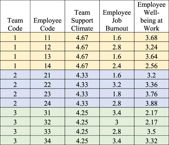
Figure 3. First cases from a multilevel data file.

Mathematically, Equation 2 tells us that γ₀₁ estimates the relationship between two team variables: team support climate (C_j) and the team intercept (β_0j), rather than between C_j and employee well-being (Y _ij). Thus, it makes sense to clarify the meaning of β_0j. In a simple regression model (Y = a + b X + e), the value for the intercept is yielded by $a = \bar{Y} - b\;\bar{X}$. Applying this expression to equation 1, we can write the following:

(5)$${\beta _{0j}} = {\bar{Y}_j} - {\beta _{1j}}\;{\bar{X}_j}$$

Thus, in our example, β_0j can be interpreted as a team mean in well-being (${\bar{Y}_j}$), once the effect of team average job burnout (${\beta _{1j}}\;{\bar{X}_j}$) has been controlled for; that is, β_0j is an adjusted team mean in well-being (Enders & Tofighi, Reference Enders and Tofighi2007; LoPilato & Vandenberg, Reference LoPilato, Vandenberg, Lance and Vandenberg2015). If we replace β_0j in Equation 2 with the right-hand part of equation 5, we get the following expression (LoPilato & Vandenberg, Reference LoPilato, Vandenberg, Lance and Vandenberg2015):

(6)$$({\bar{Y}_j} - {\beta _{1j}}{\bar{X}_j}) = {\gamma _{00}} + {\gamma _{01}} \cdot {C_j} + {U_{0j}}$$

Therefore, the coefficient that estimates the so-called “cross-level direct effect” (γ₀₁) provides an estimation of the relationship between the involved team-level predictor (in our example, team support climate, C _j) and an adjusted team mean in the outcome variable (in our example, well-being). It does not provide an estimation of the relationship between a team-level predictor (e.g., team support climate, C _j) and an individual-level outcome (e.g., well-being, Y _ij)^{Footnote 3}.

In order to avoid interpreting γ₀₁ as estimating the “effect” of a team-level variable on an individual-level outcome, several steps can be taken. First, focus should be placed on equations 2, and 6, rather than on equation 4. Equations 2 and 6 make explicit that γ₀₁ estimates the relationship between two team-level variables (a team-level predictor and a team intercept that, in this case, can be interpreted as an adjusted mean in the outcome variable).

Second, we should consider alternative ways of graphically representing the “cross-level direct effect”. In two-level designs similar to the one used in our example (e.g., individuals nested within teams), the variance in individual-level variables can be partitioned into two orthogonal components: the Between-team component and the Within-team component^{Footnote 4} (Preacher et al., Reference Preacher, Zyphur and Zhang2010). Because team-level variables can only vary across teams, they only have Between-team components of variance. γ₀₁ estimates the relationship between two components: the team-level predictor (e.g., C_j) and the Between component of the individual-level outcome involved. It is a “Between effect” (Preacher et al., Reference Preacher, Zyphur and Zhang2010). Thus, an alternative way of representing the “cross-level direct effect” is shown in Figure 4 (see LoPilato & Vandenberg, Reference LoPilato, Vandenberg, Lance and Vandenberg2015, p. 295). Note that in this representation, there is no arrow going from the team-level predictor (C_j) to the individual-level outcome (Y_ij).

Figure 4. An alternative way of representing the so-called “cross-level direct effect”.

Third, as mentioned above, γ₀₁ is a “Between effect”. Therefore, we should consider replacing its typical label of “cross-level direct effect” with the label of “Between-direct effect”. The “cross-level” term in the typical label suggests that the relationship in question runs across levels, from a higher-level variable to a lower-level one. This may have contributed to misinterpreting the meaning of γ₀₁.

Fourth, we should formulate hypotheses and interpret the associated results more accurately. Using our example, a typical “cross-level direct effect” hypothesis would read as follows: “Team support climate is positively related to employee well-being, after employee job burnout in controlled for”. However, a more precise hypothesis would be: “Team support climate is positively related to the teams’ adjusted means in well-being, once the effect of team average job burnout is controlled for”. The interpretation of the obtained results should be congruent with the hypothesis formulated and the meaning of γ₀₁ discussed above. For instance, an estimate for γ₀₁ of .21 (p < .01) would mean that there is a positive relationship between team support climate and teams’ adjusted means on well-being. We could also say that there is a positive relationship between team support climate and the Between-component of well-being.

The specification of the emergence processes involved in higher-level constructs

Multilevel models in Work and Organizational Psychology frequently involve higher-level (e.g., team) constructs that have their origin in lower-level (e.g., individual) properties. For instance, in our example, team support climate (i.e., shared team members’ perceptions about supportive relationships within the team) has its origins in team members’ individual perceptions of support in the team. To fully understand the nature of higher –level constructs, it is of utmost importance to explain the processes through “which lower-level properties emerge to form collective phenomena” (Kozlowski & Klein, Reference Kozlowski, Klein, Klein and Kozlowski2000, p. 15), that is, to explain the emergence processes involved. For instance, how do employees’ team climate perceptions become shared to form team climate? In my experience as a journal editor, associate editor, and reviewer, I have observed that this theoretical explanation is frequently disregarded in research manuscripts. When authors work with shared higher-level constructs (such as team climate), it often seems that we are only concerned about showing that there is empirical evidence to justify aggregation of individual scores to obtain an indicator of the shared construct. Then, authors generally provide evidence about inter-rater agreement (usually by means of the r _wg index; James, Demaree, & Wolf, Reference James, Demaree and Wolf1984), the percentage of variance that resides at the higher level (e.g., team), by reporting the corresponding Intraclass Correlation Coefficient (1), ICC(1), and the reliability of the team means by reporting the ICC (2). Of course, showing this evidence is operationally important, but understanding the nature of higher-level constructs and the processes involved in their emergence from lower-level properties is theoretically crucial. A brief discussion of general types of emergence processes with some specific examples can be useful to clarify this issue (for a more detailed discussion see Kozlowski & Klein, Reference Kozlowski, Klein, Klein and Kozlowski2000).

Kozlowski and Klein (Reference Kozlowski, Klein, Klein and Kozlowski2000) describe two general types of emergence processes: Composition and compilation. In composition emergence, the type and amount of the lower-level property involved is similar for all the members of the work unit. For instance, in the case of team support climate, the higher-level construct is formed from the same type of individual property (team members’ perception of support, i.e., psychological climate), and all the team members perceive similar (shared) amounts of support. Composition processes of emergence explain how convergence, sharing, and within-unit agreement develop to yield a shared unit property (Kozlowski & Klein, Reference Kozlowski, Klein, Klein and Kozlowski2000). For instance, organizational climate theory and research has identified social interaction among team members as a key process for team climate emergence (Ashforth, Reference Ashforth1985; González-Romá & Peiró, Reference González-Romá, Peiró, Schneider and Barbera2014; González-Romá, Peiró, & Tordera, Reference González-Romá, Peiró and Tordera2002; Rentsch, Reference Rentsch1990). Through continued social interactions, team members communicate, discuss, and shape their perceptions of the team. These ongoing social interactions yield a shared perception of the team that is socially constructed (Ashforth, Reference Ashforth1985). Other examples of composition processes of emergence can be found in the literature on collective mood (see Barsade & Knight, Reference Barsade and Knight2015; Kelly & Barsade, Reference Kelly and Barsade2001).

In compilation emergence, either the amount or type of the lower-level property is different, “or both the amount and type are different” (Kozlowski & Klein, Reference Kozlowski, Klein, Klein and Kozlowski2000, p. 62). To exemplify these cases, let us think first about the performance of a basketball team. To reach high performance, the basketball team needs to have a varied pool of individual skills (i.e., distinct lower-level properties). For instance, the point guard contributes to team performance by interpreting the dynamic development of the game and making strategy decisions. Likewise, the center contributes in another way by enacting different skills, such as occupying a good position under the basket and blocking the opponent’s throws. Moreover, the players can have different or similar amounts of their respective skills.

The higher-level construct of climate uniformity (González-Romá & Hernández, Reference González-Romá and Hernández2014) exemplifies a case in which only the amount of the lower-level property is different. Climate uniformity refers to the pattern of climate perceptions within the team. It represents differences in within-unit (dis)agreement in climate perceptions across work units. González-Romá and Hernández (Reference González-Romá and Hernández2014) examined three different patterns of climate perceptions of organizational support: Uniform, in which there is a single grouping of unit members’ climate perceptions; strong dissimilarity, in which distinct subgroupings within the unit are observed, located in different zones (e.g., low vs high scores) of the underlying climate facet, as occurs with polarized subgroups; and weak dissimilarity patterns, in which no more than one subgrouping of climate perceptions is found, and the members excluded from this subgroup do not form a coherent cluster. Here, the type of individual property involved is the same for all the unit members: perceptions of organizational support. However, the amount of organizational support perceived by team members can be different, which can give rise to different unit climate patterns.

Compilation processes of emergence foster variability and configuration, and they explain how different types or/and amounts of lower-level properties combine to yield higher-order configural properties (Kozlowski & Klein, Reference Kozlowski, Klein, Klein and Kozlowski2000). In the case of climate uniformity, González-Romá and Hernández (Reference González-Romá and Hernández2014) suggest that leader–member exchange (LMX) quality, demographic diversity, and organizational socialization may explain the emergence of climate uniformity. For instance, in the case of LMX, they posit that “team leaders who relate differently with distinct subgroups of team members, or have differentiated relationships with specific individual team members, may contribute to fostering nonuniform team climate patterns [strong and weak dissimilarity patterns, respectively]” (pp. 1054–1055). These differentiated relationships may produce subgroupings of team members that have different climate perceptions about the team.

As Kozlowski and Klein (Reference Kozlowski, Klein, Klein and Kozlowski2000) highlight, when a higher-level construct that has its origin in lower-level properties is used in a multilevel model, the processes that explain how the corresponding lower-level properties emerge to form a higher-level construct must be explained. Therefore, I recommend that when authors refer to a higher-level construct in the Introduction to their manuscripts, they devote enough space to this explanation about the emergent processes involved. By doing so, they will contribute to improving our understanding of the nature of higher-level constructs.

Sample size recommendations for using multilevel statistical methods

An important issue to clarify when designing an empirical research study is to establish the size of the study sample. This issue is even more relevant in multilevel studies in which sampled entities come from different levels (e.g., work teams and employees). Moreover, collecting samples composed of higher-level units (e.g., teams, departments, organizations) is generally more demanding and difficult than collecting samples of individuals (e.g., employees). Taking these concerns into account, interested researchers frequently ask questions about what an adequate size is for a multilevel study sample. Two useful sources of information for making decisions about sample size recommendations when designing multilevel studies are: (a) The results of simulation studies in which the performance of multilevel methods under varied conditions (e.g., different numbers of units and individuals per unit) is examined, and (b) power analysis tools.

González-Romá and Hernández (Reference González-Romá and Hernández2017) reviewed the aforementioned simulation studies published in recent decades. Based on their review, they suggested that when the focus is on testing cross-level direct (or Between-direct) effects and effect sizes are small-to-medium, unbiased estimates and a statistical power of at least .80 can be obtained with samples composed of 30 units and 20–40 individuals per group (Bell, Morgan, Schoeneberger, Kromrey, & Ferron, Reference Bell, Morgan, Schoeneberger, Kromrey and Ferron2014). When the interest is in testing cross-level interactions, similar results for bias and power across different effect size conditions can be obtained with samples composed of 40 units and 18 individuals per group^{Footnote 5} (Mathieu, Aguinis, Culpepper, & Chen, Reference Mathieu, Aguinis, Culpepper and Chen2012). As a last general guideline, “the studies reviewed do suggest that it is better to have more groups with fewer observations per group than the other way around” (González-Romá & Hernández, Reference González-Romá and Hernández2017, p. 193). Although helpful, these general recommendations and the more specific ones drawn from individual simulation studies must be interpreted with caution. They are based on the specific factors and conditions considered in simulations studies, which may not be generalizable to a given empirical study (Tonidandel, Williams, & LeBreton, Reference Tonidandel, Williams, LeBreton, Lance and Vandenberg2015).

The information provided by simulation studies can be complemented with the information offered by power analysis tools specifically designed for multilevel studies. These tools allow researchers to ascertain what sample size combinations (number of units and individuals per unit) will reach acceptable statistical power values^{Footnote 6}, taking into account the available information about different factors (e.g., ICC, reliability, effect sizes). These tools should be used when researchers are designing multilevel studies, before data are collected. There are tools focused on cross-level direct effects (Bosker, Snijders, & Guldemond, Reference Bosker, Snijders and Guldemond2003; Browne, Lahi, & Parker, Reference Browne, Lahi and Parker2009) and cross-level interactions (Mathieu et al., Reference Mathieu, Aguinis, Culpepper and Chen2012)^{Footnote 7}. Together, the results of simulation studies and the use of power analysis tools allow researchers to make informed decisions about sample size in multilevel designs, in addition to considering the practical constraints imposed by research work conducted with real work units (e.g., teams, departments, organizations).

Conclusion

The multilevel approach offers a more comprehensive view of complex organizational phenomena. To reap the fruits of this approach, the relationships involved in multilevel theoretical and research models have to be interpreted adequately, the nature of higher-level constructs and the processes that account for their emergence must be explained, and the design of empirical studies has to be based on informed decisions. By discussing three issues pertaining to these three points, I hope this article contributes to the improvement of multilevel research in Work and Organizational Psychology.