


Introduction
British industrialization gave rise to a sequence of events that radically transformed societies and economies. As Wrigley (Reference Wrigley2010) observed, the availability of coal and the invention of the high-pressure steam engine made it possible to overcome a period of stagnant organic growth and to consolidate a revolutionary industrial economy. One of the major breakthroughs that also took place at this time was the improvement of transport systems. New turnpike roads and waterways facilitated the movement of both people and goods. Transport speeds increased considerably and services became more reliable, allowing the consolidation of overland transport. The construction of railroads took this trend a step further, as freight and passenger costs were dramatically reduced and the demand for heavy goods transport markedly increased. The rapid expansion of the railroad network also helped to enlarge market areas and gave rise to new demands and needs. The most advanced continental economies took advantage of this to improve the integration of their markets and to develop what would soon become the industrial core of Europe. The speed and cost savings associated with these new transport systems transformed the way that people and industries operated, facilitating the transition from an industrial society to a modern economy with an increasingly important tertiary sector.
Even so, not all European countries were able to pass beyond the stage of organic growth by the mid-nineteenth century. The construction of the continent’s railroad network began with significant levels of industrialization in its core countries, but with a very different situation on the periphery. What had previously been predominantly traditional societies, now began to undergo a series of significant institutional changes that favored the development of more extensive transport networks. This also permitted the exportation of low-value-added products and the creation of the preconditions for takeoff (Rostow Reference Rostow1959). The railroads therefore arrived at a moment typified by the existence of differential stages of development and this could well have influenced their short-, medium-, and long-term impacts.
In fact, there is still an ongoing debate about the relationship between transport infrastructure and economic development. The stock of railroad infrastructure has tended to be directly correlated with economic performance, with the best-connected regions having the greatest potential for development (World Bank 2009). Leading regions tend to have the best infrastructure because they can best afford returns on initial investment. This does not, however, mean that building infrastructure in more remote and less developed regions will automatically improve their economic performance.
In the United States, where these phenomena have already been studied, the results are still subject to controversy. In a seminal contribution, Fogel (1964) stressed that the railroads did indeed contribute to the development of the national economy, but perhaps to a lesser extent than many have previously suggested. He argued that the presence of alternative means of transport, such as waterways, must also be taken into account when evaluating the economic impact of railroads. This position has, however, been largely criticized given the limited cargo-carrying capacity and enormous water consumption required to justify Fogel’s counterfactual model. In addition, it is not clear what the price of road and waterway transport would have been in the absence of the railroads (Bogart Reference Bogart, Floud, Humphries and Johnson2013). This led Donaldson and Hornbeck (Reference Donaldson and Hornbeck2016) to propose an alternative methodology for estimating market access based on railroads, roads, and waterways. They concluded that railroads had played a key role in the development of the United States.
To the best of our knowledge, this is the first study to have analyzed the effects of railroads on regional development on the periphery of Europe between 1870 and 1910. This has been possible thanks to recent efforts to create historical data sets that have allowed disaggregated analyses to be made for most of the continent. We started from the preliminary idea that the most industrialized, and therefore richest, regions would also be the ones with the greatest density of infrastructure. In line with this initial supposition, it would then be natural to assume that the least developed regions would benefit from a greater integration of their transport networks with the European core. This would have implied initiating a catch-up process typified by higher levels of development and economic convergence with the leading regions in the medium term. There is, however—as Krugman (Reference Krugman1991) has underlined—an alternative theory that states that denser and higher-quality transport networks facilitate the agglomeration of economic activity and reinforce the core-periphery pattern.
Our initial hypothesis was that the extension of the rail network on the periphery of Europe, and therefore its integration within the central market, boosted economic growth in the regions that it served. Even so, the resulting effect was insufficient to generate a process of catch-up and economic convergence between regions. The investments made to extend the rail network into the most peripherally located countries therefore largely failed to reduce economic disparities. Furthermore, when these were reduced, this did not occur in a uniform way in all the regions.
Our findings show that, overall, the total railroad mileage increased by 139 percent over this period, while GDP rose by 134 percent. In aggregated terms, this would seem to confirm the correlation between railroad infrastructure and economic growth and would be consistent with the regional income dynamics observed in Western Europe before World War I. In our preferred specification, the OLS correlation between the railroad network and per capita GDP—controlled for different variables—was statistically significant, but not very high. In terms of convergence, the results were not so clear. While the Scandinavian regions economically converged toward the core regions, the countries on Europe’s southern periphery remained wrapped in a period of major divergence with respect to the rest. In absolute terms, the inequality between states increased, and particularly during the period 1900–10. This tendency was also reproduced between the different regions of a given country, and particularly so on Europe’s southern periphery. Furthermore, the most industrialized regions tended to grow faster than the average, which perpetuated the geography of economic inequality. It is also necessary to consider the capital effect. This was particularly driven by the emergence of nation-states and resulted in the concentration of administrative and economic power in certain specific regions.
The current article is divided into six parts. After this introduction, “Historical Context” goes on to present the historical background to our study. After that, “Data” provides a brief description of the data that we used and “Methodology” describes the analytical approach that we employed. “Results” then discusses the relationship between railroads and regional economic development and the final section includes a general summary and our conclusions.
Historical Context
This section provides the historical context of the study. It is divided into three subsections that examine the railroad network, economic growth, and the combination of these two concepts.
The Railroad Network
The history of railroad construction in Europe can be briefly characterized as the sum of all the different national networks that resulted from the measures taken by each country to meet its own specific needs (Martí-Henneberg 2013). Along the way, a number of common interests emerged that also permitted the development and integration of a pan-European rail network. Political interests—such as national unification and defense—and moves to minimize transport costs—which helped to promote industry and trade—were the main factors that helped to promote such strategies (Flora Reference Flora1983; Rokkan Reference Rokkan1999; Schram 1997).
Italy presents a particularly interesting case study. Before its unification and the construction of its national railroad network, early debates were dominated by the “persistence of political divisions” and “the particularly difficult terrain” (Schram 1997: 99). Rugged terrain increased the cost of constructing and operating railroads in some regions and also of establishing connections with foreign networks. For example, due “to the unfavorable condition of the terrain,” it took nearly seven years to construct the 20-km-long section of single-track through the Simplon tunnel (1898–1905) that connected Italy to Switzerland (ibid.: 108). Despite the high cost of such projects, the postunification government still regarded railroad construction as an essential element for achieving greater political integration. This explains why the national government intervened by either providing state funding or by guaranteeing potential investors certain minimum rates of return on their investments when private initiative showed a lack of interest in a particular project. As a result, by 1910, the Italian railroad network included 14,500 km of track.
In France, the public administration was even more involved in the design of the railroad network (Mojica and Martí-Henneberg Reference Mojica and Martí-Henneberg2011; Schwartz et al. Reference Schwartz, Gregory and Thévenin2011). The constitutional principle of égalité was applied, with national legislation decreeing that each of the 95 départements should be connected by railroad (Caron Reference Caron1997). The first lines were built to speed up the transportation of troops from Paris to the northeast of the country. As in many other states, France used its economic power to encourage companies to provide rail connections to its more peripheral areas, although rugged terrain frustrated some of these plans. Even so, and as Schwartz et al. (Reference Schwartz, Gregory and Thévenin2011: 67) observed, until the very late nineteenth century, “the hilly and mountainous regions of the Massif Central, Pyrenees, and Alps were deemed all but inaccessible to steam-powered locomotion.”
In the case of Spain, the construction of the national rail network was mainly funded with French capital, although the country’s public authorities also made a number of decisive interventions. The network “was designed to radiate out from Madrid to the ports and the French frontier. It was not planned for connecting economic centers within Spain” (Milward Reference Milward2005: 61), but rather to articulate the national territory. This strategy led Pollard (1981: 207) to claim that Spain’s railroads were “built ahead of time, out of harmony with the economic stage.” However, it is also true that the orography of the Iberian Peninsula did nothing to facilitate the development of the national rail network. As a result, the most rugged regions of Spain, including the Pyrenees, the Sistema Iberico, and the Cantabrian Mountains, remained relatively underdeveloped for some time.
The German railroads were similarly regulated by the country’s public administration and were mainly developed with military requirements in mind. In consequence, the network was somewhat sparser in the southern, Alpine, region of the country (Mitchell Reference Mitchell2000). In Austria-Hungary, the railroad boom began in 1867, coinciding with the Austro-Hungarian Compromise that brought the Austrian Empire and the Kingdom of Hungary together in a single state. According to our estimations, this territory was served by only 7,700 km of track in 1870, but by about 34,200 km just before World War I. Austria-Hungary invested heavily in transport infrastructure to promote its political and economic interests (Stanev et al. Reference Stanev, Alvarez-Palau and Martí-Henneberg2017). Railroads were also seen as a quick way to mobilize troops to the country’s southern frontier (Pollard 1981; Stevenson Reference Stevenson1999).
In Scandinavia, railroad access was essentially restricted to the southern regions of the territory during its initial stages of development. In later stages, when the state authorities became more involved, railroad infrastructure was extended to connect the southern regions to the sparsely populated areas in the central and northern parts of each country. This allowed the exploitation of natural resources, such as timber and mining, and certainly helped to spur the development of their economic activity in the late nineteenth and early twentieth centuries (Enflo et al. Reference Enflo, Alvarez-Palau and Marti-Henneberg2018).
Economic Growth and Development
Although the roots of its industrialization remain subject to debate, by 1870 Britain was Europe’s most important industrial nation (Allen Reference Allen2009; Crafts Reference Crafts1985) and British industry accounted for around 34 percent of its national GDP and indeed for 25.5 percent of total European output. In France, industry also produced 34 percent of the country’s GDP, but French output accounted for a smaller share of Europe’s total output: 15.8 percent. In contrast, areas on the periphery of Europe, where industry was not so relevant, followed a different path. Industry accounted for only 17 percent of GDP in Portugal and Finland; 12 and 23 percent, respectively, in Hungary and Austria; 22 and 24 percent in Spain and Italy; and 28 percent in what was to become Europe’s fastest-growing economy: Germany (Broadberry et al. Reference Broadberry, Federico, Klein, Broadberry and O’Rourke2010). In per capita terms, these differences were even greater. In 1860, the per capita GDPs of Austria-Hungary, Finland, Italy, Portugal, and Spain were all less than 20 percent of that of Britain, while Germany’s stood at around 23 percent of that of Britain.
As a result of this uneven development, a core-periphery pattern emerged, with Britain, Belgium, and northern France at the industrial heart of Western Europe. However, with time, capital gradually flowed out from the core—and particularly from Britain—and toward the periphery. A large share of this capital was channeled in the form of foreign investment and was used to fund the construction of national railroad networks (Eichengreen Reference Eichengreen1995; Schram 1997). From 1818 to 1825, British financers granted 31 loans to entities in 17 different countries. In fact, the Rothschild family alone raised £12 million for railroad financing across Europe between 1822 and 1825 (Pollard Reference Pollard1974). As construction picked up pace across Europe, capital markets expanded, with the establishment of joint-stock houses, investment banks, and large discount houses. As Pollard (Reference Pollard1974: 61) observed: “by these means the provision of capital was shifted from the few, select, sources to the masses.”
By 1845, at least 50 French railroad lines had approached the London capital market, seeking investment funding to the tune of £80 million (ibid.). The first Belgian rail network raised capital in London, through the Rothschild family, between 1836 and 1840. It was subsequently upgraded with the support of additional capital, which was also raised in London, in 1845. In this way, British contractors obtained concessions for 770 km of track in a country with a total surface area of 30,500 km2. The Amsterdam-Emmerich line (1851–56), in the Netherlands, was also funded by a group of London investors. However, by the late nineteenth century, France had become the main source of capital. In 1854, Crédit Mobilier, which went on to finance the Union Pacific Railroad, took control of the southern Austrian railroad network, which constructed lines that reached into Serbia, Romania, and Silesia. In response, Rothschild’s Creditanstalt invested in 1,071 km of railroads in Italy. French investors also helped extend Spain’s railroad network from 500 km in 1855 to 5,000 km in 1865. By 1911, French investors owned 60 percent of Spain’s 11,400 km mainline network. In short, “Europe became one single territory open to railroad development” (ibid.: 66). These investors did not seek social prestige, but rather economic gain with government-backed, guaranteed returns on their investments. Whatever the case, the geographical repercussions of the expansion of the network included the integration of national markets and this paved the way for the eventual transition to a single European market.
This historical evidence should not surprise us. Economic historians have long regarded the period from 1870 to 1914 (the “classical gold standard”) as the high-water mark for the free-movement of capital. Using a selection of countries as examples, Obstfeld and Taylor (Reference Obstfeld, Taylor, Bordo, Goldin and White1997) showed that capital flows expressed as a percentage of GDP averaged 3.7 percent from 1870 to 1889, and 3.3 percent between 1890 and 1913, before falling to 2.1 percent during the interwar period.Footnote 1 As regards the integration of the market for investment capital, the standard deviation with respect to real interest rates (in the United States) was 4.2 percent between 1870 and 1889, and 3.4 percent from 1890 to 1913.
Europe’s market for goods also became much more closely integrated during the nineteenth century (Chilosi et al. Reference Chilosi, Murphy, Studer and Coşkun2013; Federico Reference Federico2011; Jacks Reference Jacks2005; Keller and Shiue Reference Keller and Shiue2008) and several empirical studies have explored the role played by railroads in this process. Although several forces were in play, there is apparent consensus about the relevance of railroads in the process of market integration. Along the same lines, Federico (Reference Federico2011) found that, in Europe, price dispersion for wheat and rye clearly declined after the Napoleonic wars, reaching an “all-time low” in the 1860s. Chilosi et al. (Reference Chilosi, Murphy, Studer and Coşkun2013), using a sample of 100 European cities between 1620 and 1913, concluded that distance was the major driving force behind variations in price during the prerail period. Even so, freight rates fell sharply in the 1850s and 1860s, coinciding with the extension of the railroad network.
Nonetheless, it is important to highlight the difficulty involved in disentangling the effects of the railroad from other factors. Keller and Shiue (Reference Keller and Shiue2008) found that in regions with the option of waterway transport, the shipping of cereals by water remained cheaper than by rail throughout the nineteenth century. They analyzed three factors that had a decisive influence on trade and market size: the liberalization of customs duties, agreements regarding currency payments, and transportation by train. They concluded that “the introduction of steam trains reduced price gaps by about fourteen percentage points; customs liberalizations lowered price gaps by about seven percentage points and currency agreements by about six percentage points. Thus, we found that technological change had a larger effect on market size than institutional change in the nineteenth century Europe” (Keller and Shiue Reference Keller and Shiue2008: 38–39).
The study of industrialization on the European periphery picked up momentum following the work of Gerschenkron (Reference Gerschenkron1962). More recently, O’Rourke and Williamson (Reference O’Rourke and Williamson1997) reported that the economies of the more peripherally located states began to converge with those of the industrial core in the decades immediately prior to the World War I. Even so, this process differed markedly from northern to southern Europe. In Scandinavia, the conditions in the different countries rapidly converged, while in Italy, Spain, and Portugal they did not; in fact, if anything, these countries fell further behind the core area. It could even be said that, to a certain extent, European economies formed different “convergence clubs” (Epstein et al. Reference Epstein, Howlett and Schulze2003). Using a different approach and a wider sample, Di Vaio and Enflo (Reference Di Vaio and Enflo2011) concluded that two main growth regimes could be identified: one in which most countries converged, and another in which they diverged. Most European economies fell into the first group, but we must remember that countries are usually large spatial units and that in many cases, regional data can provide us with a more detailed picture.
Railroads and Economic Development
Although it is difficult to separate the development of the nation-state from the construction of its railroad network, economic motives also played an important role in the process. While the industrial core, which mainly meant Britain and France, channeled funds; more peripherally located countries decided which lines were to be constructed. Private investors demanded assurances for their commitments, which national governments granted in the form of guaranteed returns and subsidies. Footnote 2 Political interests and state interventionism explain “the fact that railroads spread almost simultaneously in countries at very different stages of development” (Pollard Reference Pollard1974: 48), and even in regions with very different and often difficult types of terrain.
Given the rise of the nation-state across Europe, and of the associated political interests, it could be asked whether investing in railroads was misguided. Since the 1960s, economic history has, however, tended to examine this question from only one specific angle: that of social savings. Social savings can be proxied as the difference between the freight rates for prerail transport and those for railroad multiplied by the total volume of rail traffic. In this respect, Fogel (Reference Fogel1962) and Fishlow (Reference Fishlow1965) argued that US national income for the years 1860 and 1890 would only have been reduced by a few percentage points if the country’s railroads had never been built. For England and Wales, Hawke (Reference Hawke1970) reported social savings of 4 percent of GDP for 1865, whereas Leunig (Reference Leunig2006) suggested that the railroads saved around 5 percent of British GDP. Using a similar approach, Herranz-Loncan (Reference Herranz-Loncan2006) suggested that railroads had a smaller impact on nineteenth-century Spain than they had had in Britain. This could be indicative of differences between the dynamics affecting the states at Europe’s industrialized core and those present in areas with more rural occupational structures.
Nonetheless, the concept of social savings, and the associated methodology, remains shrouded in controversy. As Bogart (Reference Bogart, Floud, Humphries and Johnson2013) points out, it is not clear what the price of road or waterway transport would have been in the absence of the railroads, particularly bearing in mind the fact that traffic congestion—and its associated diseconomies of scale—would have been significantly greater. Secondly, social savings ignore the demands that the railroads placed on the iron and steel industries and on the other transport innovations that span off from railroad development. Thirdly, it must be underlined that this approach ignores aspects related to the spatial redistribution of economic activity, which could have produced more agglomerations and exacerbated existing inequalities in regional income. Bearing all these considerations in mind, Crafts (2004) offered an alternative approach based on the theory that the productivity of a given economy is equal to the productivity of each of its sectors multiplied by their share of national GDP. Crafts (ibid.) calculated that the growth in productivity associated with railroads in Britain contributed 0.05 percent to the growth in per capita income between 1830 and 1860, which was equivalent to a social saving of 1.5 percent of GDP over the whole period. However, this method underestimates the contribution of railroads to this process because it ignores gains in productivity resulting from those made from displacing previous forms of transport.
Pursuing this line of research, recent studies have made more intensive use of a combination of spatial analysis and econometric techniques. Atack et al. (Reference Atack, Fred Bateman and Margo2010) used a binary variable to capture railroad access in the Midwest of the United States, finding that it played a significant role in promoting urbanization during the 1850s. However, this did not prove so relevant in terms of its influence on population density. In a related work, Atack et al. (Reference Atack, Haines, Margo, Rhode, Rosenbloom and Weiman2011) examined the relationship between railroads and factory status, finding that railroad access had a generally positive impact. Atack and Margo (Reference Atack and Margo2011) similarly explored a mechanism through which access to the network might also affect economic activity: cultivable land. They suggested that, as a whole, at least a quarter—and possibly up to two-thirds—of the increase in cultivable land in the American Midwest could have been attributable to the construction of railroads. Although these studies pioneered the use of geographic information systems (GIS) to digitize maps and related sources, they also used a differences-in-differences approach to evaluate the relative impact of the railroads.
Donaldson and Hornbeck (Reference Donaldson and Hornbeck2016) went a step further and developed an approach to estimate the aggregate impact of the railroads. To do this, they derived a proxy for market access based on data relating to railroad, road, and waterway transport and examined the degree to which greater market access, resulting from the expansion of the railroads, affected agricultural land values in the United States between 1870 and 1890. Briefly stated, they concluded that railroads were essential for the spread of agriculture in the United States. Furthermore, they calculated that agricultural land values would have declined by 60 percent if the railroads had not been built (ibid.). In short, it seems that a market access approach suggests a substantially greater effect than the social savings method.
Koopmans et al. (Reference Koopmans, Rietveld and Huijg2012) studied how changes in accessibility affected population growth at the municipal level in the Netherlands. They showed that rail accessibility was positively correlated with population growth, particularly from 1880 onward. Even so, according to their findings, the overall impact seemed to be rather modest. A complementary approach was used by Alvarez et al. (Reference Alvarez-Palau, Franch and Martí-Henneberg2013) to analyze the impact of railroad access on population growth in England and Wales between 1871 and 1931. The results showed the importance of the degree of access to railroad stations and its role in conditioning urban growth. Civil parishes with two or more stations grew more than those with only one, while the latter grew more than those without a railroad station. Berger and Enflo (2015) studied towns to detect a positive, and statistically significant, relationship between railroad access and population growth in Sweden. Although their findings basically reflected the relocation of economic activity, it is worth noting that settlement populations showed no tendency to converge during the twentieth century, despite a notable expansion of the rail network.
Empirical studies have also examined several other contexts. For instance, Donaldson (Reference Donaldson2018) explored the relevance of rail access in colonial India (1870–1930), finding that railroads reduced price gaps, promoted trade, and increased real agricultural income per acre. In Sub-Saharan Africa, Jedwab and Moradi (Reference Jedwab and Moradi2016) concluded that railroad access has had a substantial impact on the spatial distribution of economic activity and that these effects may persist in the long run.
Most of these studies have been based on individual countries. One exception to this rule was that of Jedwab and Moradi (ibid.), which used Sub-Saharan African countries to supplement other work carried out in Ghana. As regards Europe, there is a vast literature, but a good deal of this is based on specific countries or regions. In fact, very few empirical studies have used European regions as their spatial units of analysis. The only attempt to do this was a study carried out by Caruana-Galizia and Martí-Henneberg (Reference Caruana-Galizia and Martí-Henneberg2013). They put together data for Austria-Hungary, France, Germany, Italy, Spain, Sweden, and United Kingdom in the form of a preliminary report and then presented several research ideas.
The current study therefore provides the existing literature with a broader scope. GIS have enabled us to digitize maps and to construct the proxies for railroad infrastructure that we present below. While most of the cited works have restricted their analyses to urban and population growth, in this article we have used historical estimates of GDP for 287 regions and four countries. This has allowed us to exploit cross-section variation over the whole study period.
Data
This article combines railroad data with population and historical estimates of GDP from 1870 to 1910. The variables were disaggregated at the subnational level and mapped using GIS. European regions were used as the spatial units of analysis, although the main focus was placed on regions in peripherally located countries. In this case, it is relevant to underline the relative stability of Europe’s historical geography since 1870 and, in particular, of the countries in our sample.
The Railroad Network
The railroad data used here were obtained from the Historical Geographical Information System of Europe (HGISE) project. This was led by Jordi Martí-Henneberg and investigated how transport technologies have contributed to European integration from 1825 through to the present day. The primary sources consulted were Cobb’s Railways of Great Britain: A Historical Atlas; the Thomas Cook travel series; John Bartholomew and Son’s map series; the Historie Chronologique des Chemins de Fer; and various other national-level sources, which are all detailed in Morillas-Torné (Reference Morillas-Torné2012). All these sources were used to compile a GIS of Europe’s broad-gauge railroads at 10-year intervals.
Standard gauge (1,435 mm) railroad tracks were digitized to reconstruct the mainline railroad network. In the case of the Iberian Peninsula though, the gauge was slightly wider (1,668 mm). The same occurred in the former USSR, including Finland, where yet another gauge width was used (1,524 mm). As international connections already existed, the only important issue relating to cross-border travel was the need to stop to change carriages. There were also other, nongauge-related reasons for trains stopping at international borders. These included differences in electrical power voltages and signaling systems. Crossing a national border therefore often resulted in delays.
Narrow gauge tracks (typically 1,067 mm) were mainly used to cover short distances and were predominantly found in Southern Italy, Switzerland, Belgium, Norway, and the most peripheral areas of Spain. Even so, they only constituted a relatively small fraction of the total network, so we did not include them in our study.
If we consider the period 1840–70 to have corresponded to the first wave of railroad construction (mainly in the United Kingdom, France, and Germany), the period that we chose to study would have corresponded to the second wave. Figure 1 traces the evolution of the total length of railroad track in operation in different countries. The United Kingdom, France, and Germany already had dense rail networks before 1870, while in more peripheral countries, railroad construction started later, and at a slower pace. Of the countries in this second group, Italy, Spain, and Sweden had already accumulated significant total mileages of track by 1910. In contrast, Austria-Hungary, Finland, Norway, Portugal, and Denmark lagged behind, with much less infrastructural stock.
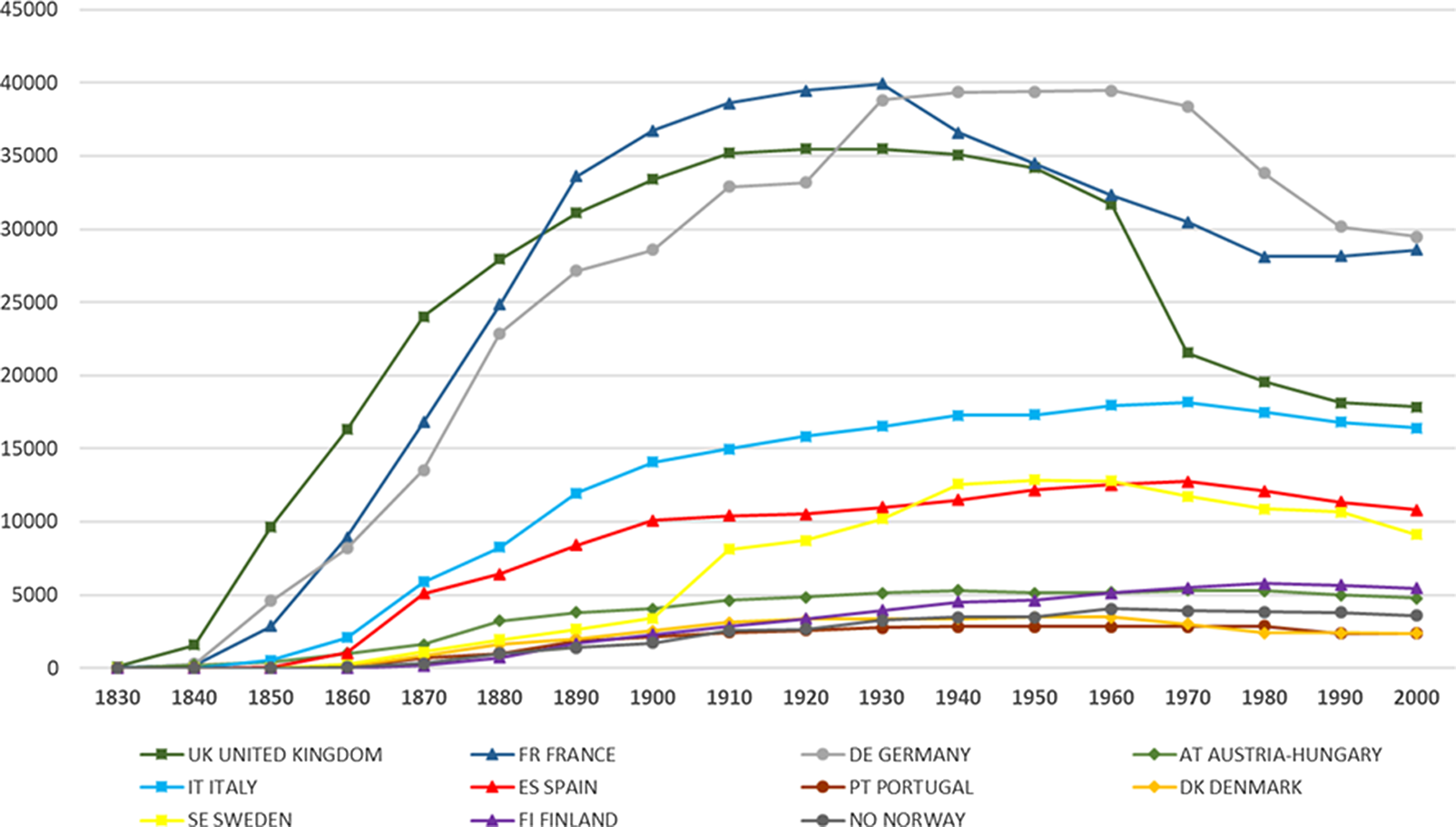
Figure 1. Length of railroad track: Comparison by country, 1830–2000.
Source: Own work (see data section).
Gross Domestic Product
Regional population and historical estimates of GDP were collected from the Historical Economic Geography of Europe project coordinated by Joan Rosés and Nikolaus Wolf (Reference Rosés and Wolf2019). In particular, we used their estimates for Austria-Hungary, Denmark, Italy, Finland, Norway, Portugal, Spain, and Sweden.Footnote 3 The majority of these countries had enough data to cover the whole study period; the exceptions were Finland and Portugal, whose historical estimates began in 1880 and 1890, respectively. To analyze comparable data for the whole period, we decided to extrapolate backward to the year 1870, assuming the existence of the same economic structure as in the first year, using accurate data and Maddison’s estimates (Maddison 2007). The same interpolation procedure was applied for Norway during the period 1880–90.
We also compiled additional data for the United Kingdom, France, and Germany to obtain a benchmark sample. The British data were processed by Crafts (2005), the French data were obtained from Bazot (Reference Bazot2014), and the German historical estimates of regional GDP were provided by Caruana-Galizia and Martí-Henneberg (Reference Caruana-Galizia and Martí-Henneberg2013). Although the benchmark sample provided extensive coverage for most of Europe, for some countries we were unable to find available data corresponding to the regional scale. In those cases, to avoid any possible selection bias, we included national estimates in the sample. This enabled us to add data for Belgium, the Netherlands, Luxemburg, and Switzerland to the data set.Footnote 4
One major concern relating to all these estimates was their comparability: they were based on current prices and derived from calculations involving different national currencies. Following Caruana-Galizia and Martí-Henneberg (Reference Caruana-Galizia and Martí-Henneberg2013), we standardized our historical estimates of regional GDP, presenting them at 1990 Geary-Khamis dollar values. The different country-based series were therefore converted based on a benchmark year derived from Maddison (2007). The results obtained proved insensitive to the choice of benchmark year.
Descriptive Statistics
As shown in figure 2, the first wave of railroad construction took place between 1840 and 1870. In 1850, fewer than 30 percent of the different regions had access to the railroad. However, by 1870, things had completely changed, with almost 80 percent having railroad access. In our study period, 1870–1910, the percentage of connected regions continued to grow, with rail coverage reaching up to 97.3 percent. This meant that we can state that all the regions of Europe were effectively interconnected by rail before 1910; as a result, the continental market could be considered to have become fully integrated by this date. However, if we look at the total GDP share of the 20 percent of regions that lacked railroad access in 1870, we see that the sum of their GDPs barely amounted to more than three percent of the combined total for all of the regions.
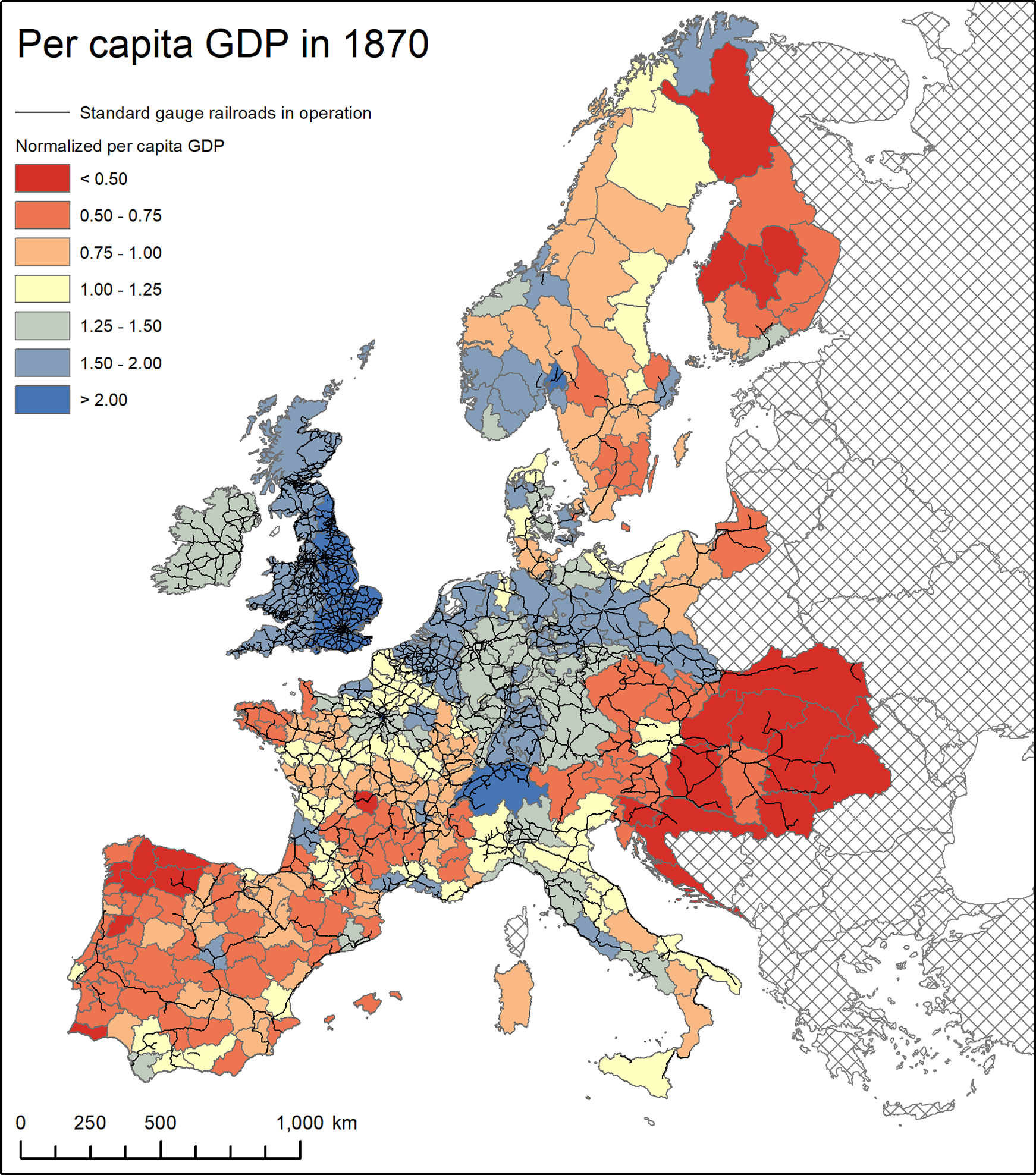
Figure 2. Per capita GDP and the railroad network in 1870 (normalized by the average).
Source: Own work (see data section).
Table 1 summarizes the evolution of per capita GDP and railroad density. It is possible to observe substantial contrasts in railroad density between some countries and others. The core countries had all reached values of 30 meters of stock per square kilometer by 1870. However, the more peripherally located countries had much lower values. Variations within countries were also relevant, with coefficients of variation in 1870 ranging from 2.73 in Norway to 0.42 in Germany. However, these eventually declined, and by 1910, the respective ranges for Norway and Germany were 1.08 and 0.19. This cross- and within-country variation showed that railroad access was already significant in some areas by 1870. This pattern subsequently converged as more railroad track was constructed. Similarly, we found considerable variations both between and within countries with regard to per capita GDP. Switzerland had an average per capita GDP of $6,709 in 1870, while in Austria-Hungary, the mean was only $1,324. The coefficient of variation ranged from 0.41 for France to 0.16 for Italy. By 1910, per capita GDP had grown considerably, and so had regional inequality within countries. Spain had a coefficient of variation of 0.40, France of 0.35, and Norway of 0.31. This is a very relevant finding and highlights the fact that national aggregates may mask considerable heterogeneity within a given country. This is, in itself, an argument in favor of conducting more spatial studies using data relating to the regional scale.
Table 1. Country-level descriptive statistics

Sources: See text.
All these descriptions can also be highlighted geographically. Figure 2 shows regional per capita GDP combined with the railroad network in 1870. Certain patterns are evident from the map. In line with table 1, the core countries had denser rail networks as well as higher levels of per capita GDP. This can be seen in the United Kingdom, Belgium, the Netherlands, Luxemburg, Germany, and Switzerland. However, Austria-Hungary and the Scandinavian and Iberian peninsulas exhibited very low levels of both per capita GDP and railroad density. The only exception in this second group was Norway, which exhibited important levels of per capita GDP, despite having a very low railroad density. Denmark, Italy, and France could be considered examples of intermediary situations, having both leading and lagging regions. Whatever the case, what seems clear is the correlation between railroad density and per capita GDP on the continent.
In 1910, the situation was a little different, as shown in figure 3. Norway and Denmark had, by this time, achieved important levels of per capita income, which clearly situated them above the European average. Sweden and Finland considerably improved their positions with respect to the initial period, although only a few Swedish regions were above the European average. Meanwhile, Austria-Hungary, Italy, Spain, and Portugal experienced relative losses in per capita income. In the case of the Iberian Peninsula, this situation was particularly evident along the west coast and in the interior.

Figure 3. Per capita GDP and railroad network in 1910 (normalized by the average).
Source: Own work (see data section).
All considered, it seems evident that the core regions of Europe maintained their leading position in terms of per capita income. The peripheral regions, however, continued to follow very different paths. While a process of economic convergence began along the northern periphery, on the southern periphery, the tendency was for a continuation in divergence from the core. These preliminary results seemed to fit in with our initial hypothesis that the integration of the railroad network did not follow a homogeneous process of economic convergence between the center and the periphery.
Additional Variables
Although playing only a secondary role in the creation of our theoretical model, the present work also benefited from a series of additional variables that helped us to monitor the proposed correlations.
Firstly, we had data on the population of each of the regions from 1870 until 1910, at 10-year intervals (Martí-Henneberg Reference Martí-Henneberg2005). In aggregated terms, the population grew by 114 percent over the whole period. Even so, if this period was characterized by anything, it was by its deep-seated demographic restructuring, which can largely be explained by mass migrations between different parts of the continent (Pollard Reference Pollard1974). This variable was not incorporated into our model in absolute terms, but it was taken into consideration when calculating the per capita GDP variable.
In parallel, a series of geographical variables were created that did not change over time. For example, coastal regions were identified using a dummy variable. A series of regions that contained capital cities were similarly identified. We then calculated the average distance from the different regions to the nearest major river. To capture location, we introduced the concept of centrality, which measured the distance between the centroid of region i and the centroid of the whole of Europe; geographical distance has often been used for this purpose in economic geography (Head and Mayer Reference Head and Mayer2006). Finally, we estimated average elevation and also the average slope of the terrain. These last two variables were generated using the Digital Elevation Model of Europe (Eurostat 2014).
Methodology
In line with other cases mentioned in the literature section, we assumed a clear correlation between railroad density and per capita GDP. However, our goal was to go a step further and to try to explain changes in regional standards of living based on infrastructural stock. We therefore began with the following equation:
 $$\Delta {y_{i,t - 1 \to t}} = \alpha + \beta \cdot{y_{i,t - 1}} + \delta \cdot Rw{D_{i,t}} + {\theta _i} + {\mu _i} + {\epsilon_{i,t}}$$
where Δyi,t is the log difference in per capita GDP for each region i, and year t. The variable y i,t−1 accounts for the per capita GDP of region i, and year t-1, using a logarithmic transformation. Railroad infrastructure is proxied with railroad density (km/km2), which is the length of railroad track over the total area of region i, in year t. The term θ i, represents the country fixed-effect. Similarly, μi controls other fixed effects in each region. These include whether it contains the national capital; if it is a region containing a coastal area; its relative centrality (measured in distance from the European centroid); its distance from a major river; its average elevation; and, the average slope. Finally, ε i,t represents the error term.
We understand that there is general consensus within the academic community as to the higher level of development found in the areas that have the greatest amount of infrastructure. However, in this article, we are not primarily interested in the correlation in itself, but rather in disentangling the influence that the existing infrastructure and any new developments may have on regional development. We therefore propose breaking down the railroad term used in the equation into its lagged value in t-1 plus the growth experienced between t-1 and t in absolute terms:
 $$Rw{D_{i,t}} = Rw{D_{i,t - 1}} + \Delta Rw{D_{i,t - 1 \to t}}$$
Substituting (2) in equation (1), we obtain our baseline equation:
 $$\Delta {y_{i,t - 1 \to t}} = \alpha + \beta \cdot{y_{i,t - 1}} + \delta '\cdot Rw{D_{i,t - 1}} + \delta ''\cdot \Delta Rw{D_{i,t - 1 \to t}} + {\theta _i} + {\mu _i} + {\epsilon_{i,t}}$$
Despite introducing controls for country and regional heterogeneities, the simultaneity between infrastructure stock and development remains an issue. It seems evident that the two variables grew in parallel and that there could have been a certain amount of interaction between them. Even so, we have not sought to tackle the problem of simultaneity and causality here. Instead, the current work is presented from an exploratory perspective, leaving the door open for more in-depth statistical analysis in future works.
Once our model had been empirically tested, we went on to incorporate a series of complementary techniques to explore our results at the national and regional levels. These techniques have been described throughout the text, as and when they have been used.
Results
Table 2 presents the main results. For the regression, we used a cross-section containing 291 observations, referring to 287 regions and four countries. We divided our estimates into three parts. First of all, we looked at the first 20-year period in [1] and [2] and tried to explain per capita GDP growth between 1870 and 1890. Secondly, we focused on the second period, from 1890 to 1910, in [3] and [4]. Finally, we extracted the results for the whole period in [5] and [6], considering a 40-year window. In the odd-numbered columns, we only correlated per capita GDP growth with the lagged value of per capita GDP, without any further controls. We did this in search of a β-convergence phenomenon. The even-numbered columns show the whole regression resulting from equation (3), incorporating all the controls.
Table 2. Empirical estimates of growth in per capita GDP (log diff): Baseline equation

* p < 0.05; ** p < 0.01; *** p < 0.001.
The lagged values for per capita GDP showed a low and negative correlation with changes in per capita GDP; the R-square values also remained below 0.1. The presence of railroads, proxied with railroad density, exhibiting a positive and statistically significant relationship in all the periods studied, with this being particularly evident in the second period (1890–1910). Although the magnitude of this tendency was not large, the results obtained were robust and supported the argument that having more railroad infrastructure produced economic activity (Atack et al. Reference Atack, Fred Bateman and Margo2010; Donaldson and Hornbeck Reference Donaldson and Hornbeck2016; Jedwab and Moradi Reference Jedwab and Moradi2016). Growth in railroad density did not, however, seem to be statistically significant in the short term. Unlike railroad density, the growth in railroad density showed a high correlation during the first period, but dropped off considerably thereafter.
The Lack of Convergence between the Core and Periphery
One of the hypotheses that we proposed was whether the integration of the European rail network would have brought with it a process of economic convergence between the industrialized center and the periphery. If we wanted to analyze this effect, it was necessary to carry out two checks. Firstly, it was necessary to check the β-convergence results presented in table 2. The β-convergence is a condition that is necessary, but not sufficient, for convergence between regions and indicates that the poorer regions are growing faster than the richer ones. The negative value of the correlation between the growth in per capita GDP and in per capita GDP in the initial period pointed in this direction. This negative sign was maintained in all our specifications. This reinforced the idea that, on average, the poorer regions were catching up with the others.
This means of checking does, however, imply a number of shortcomings. If the regional economies have not yet reached the Steady State, there is no reason why convergence should take place in absolute terms. This argument led us to the second check: absolute convergence or σ-convergence. To test for potential σ-convergence, we decided to represent the coefficient of variation of the main variables involved in the correlation. The results, as normalized for 1870, are shown in figure 4.

Figure 4. Evolution of the coefficient of variation of the variables per capita GDP, GDP, population, and railroad density.
Source: Own work (see data section).
The previous figure shows a series of highly clarifying results. If we take the 1870 values as being fixed and equal to one, we can observe the evolution of the different variables used in the study. As expected, the coefficient of variation of the railroad density variable gradually decreased. Extending the railroad network toward the peripheral regions produced greater integration between the center and the periphery. This extension increased the degree of railroad density in the poorest regions and therefore facilitated their convergence with the values previously attained in the core regions. In contrast, the results in terms of GDP, population, and per capita GDP showed different patterns. The coefficient of variation of the three variables showed a rising tendency and tended to exceed a value of one. This indicates that the disparities between the richest and the poorest regions tended to grow throughout the period studied. It could therefore be said that there was convergence in terms of infrastructure, due to the integration of the network, but divergence in economic terms. The poorest regions not only failed to catch up with the richest ones in absolute terms, but regional disparities even increased.
Uneven Development in Countries on the European Periphery
In this section, we wish to identify differential behavior between peripheral countries and to investigate the potential existence of “convergence clubs” (Epstein et al. Reference Epstein, Howlett and Schulze2003). Figure 5 shows the growth in per capita GDP in relation to the initial stock of infrastructure and the growth in this stock in each country.
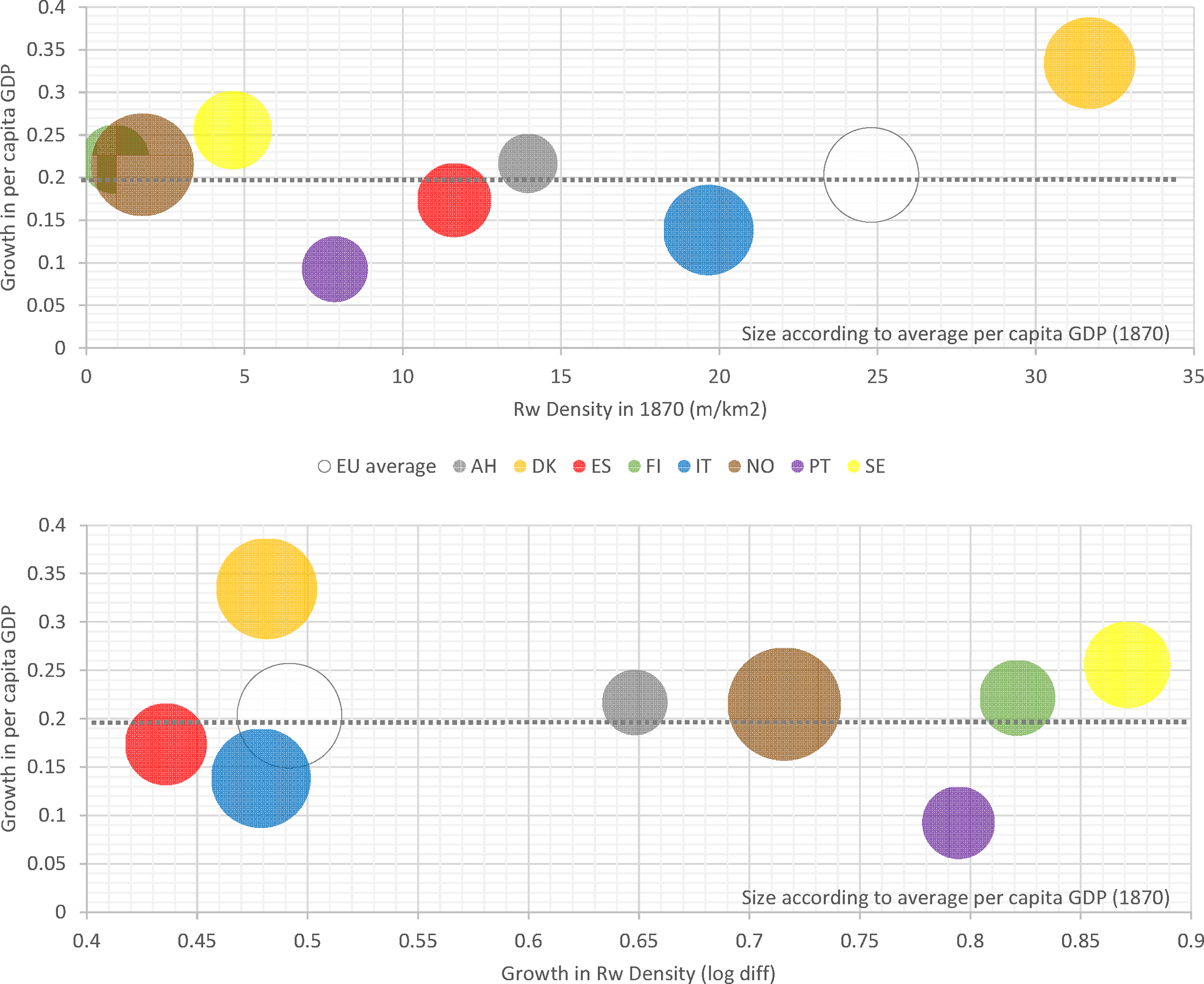
Figure 5. Growth in per capita GDP vs, railroad network in 1870 (above), and growth in railroad network, 1870–1910 (below). Dot size reflects the initial value of per capita GDP in 1870.
Source: Own work (see data section).
The first conclusion that can be drawn from the upper panel of figure 5 is that there were tremendous differences between some countries and others. Looking at the relative position of the European average (24.8, 0.20), it is easy to note the economic backwardness of the countries on the periphery. Only Denmark initially had a higher railroad density than the European average. Furthermore, in terms of per capita GDP in 1870, only Denmark and Norway had average levels of per capita income that exceeded $3,450. Following this reasoning, it would be logical to consider that Denmark formed part of Europe’s core in 1870. Its more northerly location and its historical ties with the Scandinavian countries did not hide a series of differentiated development patterns. The rest of the Scandinavian countries exhibited similar patterns, which we could consider as clustered. Although Norway would no doubt have attained an above average level of income by 1870, it is equally true that the expansion of its railroad network still remained at a relatively embryonic stage. Sweden, Finland, and Norway had levels of railroad density of less than 5 meters per square kilometer. This circumstance could be explained by their extensive territories combined with their extremely low levels of population density. Whatever the case, the interesting point is that these three countries exhibited per capita GDP growth rates that were above the European average. In contrast, the countries on the southern periphery showed a pattern of behavior that was very different. Although they exhibited considerably greater railroad densities than the Nordic group, their regional economic growth values were considerably lower. Italy, with a railroad density of 19.7, came very close to the average. The same was true of its initial levels of income, but its growth rates were 30 percent below the average. The same occurred in the cases of Spain and Portugal, with respective growth rates of 0.17 and 0.09 (0.4 percent and 0.2 percent in annual terms). In fact, Portugal was the country with the greatest economic divergence from the core in the study period. Finally, Austria-Hungry could be considered a unique case. Although its average railroad density, of 13.9 km/km2, was similar to the overall average, its per capita income was far inferior and its growth rate was only slightly above the average.
The lower panel of figure 5 reveals the second part of the story. In this case, there is a repetition of what was seen in the previous figure but using the growth of the railroad network variable along the horizontal axis. The intention behind this analysis was to explain the relationship between the growth in railroad density and average economic growth.
The average increase in the size of the railroad network remained below 0.5 (1.2 percent per year), with an average economic growth of 0.20 (0.5 percent per year). Spain, Italy, and Denmark were the only countries with lower railroad construction ratios. As previously mentioned, the Danish case could be explained by the country forming part of the core in terms of its development before 1870. Whatever the case, its economic growth was considerably greater than the average. Spain and Italy, however, were examples of tendencies in the opposite direction. Both countries were underdeveloped in 1870 and their growth rates for the study period showed a tendency to diverge from the industrialized core. In the case of Portugal, even with a notable increase in railroad density, growth rates remained extremely poor. In contrast, the success stories included the evolution of the Scandinavian countries whose railroad densities increased by more than 1.5 percent, while they experienced economic convergence with the core.
All in all, the existence of various different “clubs of differential convergence” seems evident (Epstein et al. Reference Epstein, Howlett and Schulze2003; O’Rourke and Williamson Reference O’Rourke and Williamson1997). The regions belonging to the Scandinavian countries grew at notably higher rates than the average and, therefore, from an economic perspective they tended to converge with the core. The countries belonging to the southern periphery, however, exhibited very low growth rates, which meant that they tended to diverge from the core.
Differential Effects within Countries
With the previous analyses, we were able to demonstrate the absence of economic convergence in absolute terms and the creation of “convergence clubs.” In this section, the aim is to go one step further and to explore what regional data shows at the national scale. Figure 6 shows average annual economic growth for each of the regions analyzed and also the extension of the railroad network between 1870 and 1910.

Figure 6. Geographical distribution of growth in per capita GDP and railroad network expansion between 1870 and 1910.
Source: Own work (see data section).
The figure shows the regions that had the highest average levels of growth in shades of dark blue, while the orange and red tones indicate very low levels of growth and even decline. A quick look at the map allows us to note a major concentration of growth around the European core, but also in the northern periphery. The orange and red tones, by contrast, are mainly concentrated in the south and east.
In railroad terms, it is possible to observe the expansion that took place toward the more peripheral areas. Many of these areas passed from having no infrastructural stock in 1870 to being fully integrated into the European network. This was not only the case of the Spanish, Portuguese, and Italian regions in the southern periphery, but also of those in Norway, Sweden, and Finland in the north.
If we analyze these cases in detail, it is possible to appreciate the regional dynamics much better. We should first focus our attention on the Nordic countries. Denmark, as previously mentioned, exhibited patterns similar to those of the core. By 1870, it already had rail connections to all its regions, with the obvious exception of maritime connections. Its economic development was also evident. Copenhagen, East Zealand, East Jutland, and Bornholm had the highest growth values in the whole of Europe, with these all being more than 1 percent. In the case of Norway, the railroad network mainly extended during the period studied. In fact, in 1870, the country only had relevant infrastructure around Oslo and Trondheim. It was possible to observe important growth along the southeast and northwest coasts, which were areas with a high concentration of mining activity (Enflo et al. Reference Enflo, Alvarez-Palau and Marti-Henneberg2018), although the highest rates were registered in Hedmark. There was, therefore, compensated growth between the northern and southern regions of the country. In Finland, the situation was similar. In 1870, the railroad network only reached the outskirts of Helsinki, before subsequently extending toward the main cities. Then, in a second phase, it extended toward the north to form an integrated national network. The beginning of new economic activities based on the extraction of natural resources could explain the greater rates of growth experienced in the northern regions. In Sweden, however, the situation was different. By 1870, the country had a first rail network, which connected the cities of Stockholm, Gothenburg, and Malmo. Although the network did extend toward the north, the greatest rates of growth were concentrated in the southern part of the country and particularly in those corridors that had had railroad connections since 1870. It should be noted that in all three cases, the cities described were located on the coast and therefore also enjoyed maritime connections.
If we focus our attention on the southern periphery, we find a very different situation. In the case of Italy, there was already a railroad network connecting the north and center of the territory in 1870. However, the integration of the south did not take place until later. It was possible to observe high levels of growth in the north—in Liguria, Piedmont, and Emilia—but much more modest levels in the rest of the recently unified national territory. Spain presents a similar case. The railroad network already had several connections during the initial period that connected the state capital to the main cities on the coast. This did not, however, directly lead to growth in the connected regions. In fact, economic growth only occurred in the north of the peninsula, and especially in Galicia, the Basque Country, and Catalonia. In economic terms, the geographic difference observed in Spain—as in Italy—was a result of a higher level of industrialization in the north. The central and southern areas, where the primary sector had a greater importance, had low growth values, with these even being negative in regions such as Murcia. In Portugal, the situation was similar to that in Spain, with the difference that there was nowhere with high rates of economic growth. This was so to the extent that Portugal had 6 of the 20 regions with the lowest rates of growth in the whole of Europe.
Taken together, these results show that differences in national dynamics were important. Neither the extent of the railroad network nor that of economic development were uniform. Martí-Henneberg (2013) showed how the governments of the different states took advantage of the creation of their respective railroad networks to integrate their national territories; this was a move which could have affected their economic development. Major investment in previously underproductive railroad network could have compromised the public purse and therefore limited the potential for stimulating productive activity. One simple way to explore whether this was the case would be by examining the relative positions of the regions that included capital cities at the beginning and end of the period studied. Table 3 shows the changes in the rankings of per capita GDP and railroad densities between 1870 and 1910 for each of the capital regions.
Table 3. Relative position and changes in economic and infrastructural rank of capital regions between 1870 and 1910

Sources: See text.
The results obtained are certainly thought provoking. Both in terms of railroads and economic development, the regions containing national capitals exhibited performance values that were considerably above their national averages. Beyond the utopic models of centrality of Paris and London, we see that Oslo and Helsinki followed similar patterns. The two capitals had the best values for railroad density and led regional economic development in their respective countries. We shall now examine the cases of Vienna, Stockholm, and Lisbon. There, the regional capitals led economic development, although their railroad networks did not show such clear signs of radial design. The Swedish case was particularly significant, as it lost up to 11 ranking positions in terms of railroad density. Rome and Madrid are cases that deserve a category of their own: their regions had a good amount of railway infrastructure—albeit, not the best—but they lost relative position in terms of economic development. Madrid, for example, lost as many as three positions in the ranking in favor of the industrialized regions on the periphery of the Iberian Peninsula.
Whatever the case, the results presented in the table highlight how, in more than 75 percent of cases, the capital led the economic development of each country. This result shows that the agglomeration effect did not only occur at the European scale but also at the national scale. The emergence of the railroad network within a context of nation-state building had a major impact, not only on the conception of the network but also on the redistribution of economic activity. The division between the center and the periphery was also accentuated by the capital effect.
Conclusions
In this work, we have examined the relationship between railroad integration and regional economic development in Europe between 1870 and 1910. To do this, we used a database including 291 regions (287 national regions and 4 countries), with information on railroad density and per capita GDP. Our working hypothesis was that the unfurling of the railroad network toward the European periphery contributed to growth but did not bring with it an economic convergence effect from poorer to richer regions. Our results also demonstrated our initial supposition: although there was a positive correlation and statistically significant relationship between railroad density in the initial period and growth in per capita GDP, the size of this effect was relatively small for the period as a whole. The impact of railroad construction on the economic growth variable did not seem to be statistically significant in the short term.
In the case of economic convergence, we tested two indicators. We studied the β-convergence between the lag values for per capita GDP at the beginning of the study period and the economic growth experienced. The coefficients were similar for all the specifications, showing a negative sign and similar values in terms of magnitude. This implied larger average growth in regions with lower initial per capita GDP values. When we studied the σ-convergence, the results differed notably. Studying the coefficient of variance of the railroad density and per capita GDP variables, we noted a clear convergence in terms of infrastructure, but a divergence in absolute economic terms.
Analyzing the performance of each of the countries on the periphery, we observed clustered patterns. Sweden, Finland, and Norway would form part of a first “club of countries” that began with a very low network density but experienced notable economic growth. Italy, Spain, and Portugal would be examples of the opposite trend, with fairly dense initial networks, but with less economic development during the period studied. Denmark and Austria-Hungary, in contrast, were not members of either of these “convergence clubs” and each followed their own dynamics.
In national terms, we observed that the three Nordic countries followed a similar pattern with respect to the construction of their respective railroad networks. All their networks began around main cities, located in the south of their territories, and later expanded northward to help exploit the available natural resources. This allowed gradual growth and made it possible to limit regional disparities. In Southern Europe, however, the situation was very different. With a population structure highly concentrated along the coast, the railroad network was designed as a tool for integrating the whole of each national territory. Even so, the economic response was to promote the most industrialized regions in the north instead of the whole of the national territory. In national terms, the major role played by the capitals of the recently created nation-states was also demonstrated. In 75 percent of cases, the capital regions led the regional economic development of their respective countries.
Finally, the authors understand that this study should be regarded as a starting rather than an end point. It shows how the availability of improved transport infrastructure could not only have stimulated growth but could also have encouraged the agglomeration of economic activity. Further exploration of population and historical GDP may open up new avenues for future research, perhaps even investigating smaller spatial units thanks to the use of GIS. In econometric terms, the completion of the sample to create a balanced panel starting from 1850, the homogenization of regional GDP estimates, exploring the causality and simultaneity between variables, and making further improvements in the control variables, are the main challenges that still remain to be met in the short term.
Acknowledgments
We would like to acknowledge Paul Caruana-Galizia for his work in the early stages of this paper. We also would like to thank Mateu Morillas for his work as research assistant, as well as Jørgen Modalsli, Nicholas Crafts, Frank Geary, and Julio Martinez-Galarraga for helping with our research. Funding was provided by Ministerio de Economía y Competitvidad (ECO2015 65049 C12-1-P; ECO2015 71534 REDT), Ministerio de Ciencia, Innovación y Universidades (PGC2018-095821-B-I00), and University of Lleida-INDEST.


