Introduction
Living organisms are usually distributed neither uniformly nor randomly, but form all kinds of spatial structures (Legendre and Fortin, Reference Legendre and Fortin1989). Understanding these spatial structures and the spatial heterogeneity – i.e. the tendency of things to be unevenly distributed in space (Dutilleul, Reference Dutilleul1993) – they create, is of vital importance to plant ecologists, particularly as the distribution of viable seeds in the soil affects the probability of a plant establishing in a given place (Thompson, Reference Thompson1986). Indeed, as seedlings may be recruited from the seed bank in small gaps in the vegetation of grasslands (Pakeman et al., Reference Pakeman, Attwood and Engelen1998; Kalamees and Zobel, Reference Kalamees and Zobel2002; Pakeman and Small, Reference Pakeman and Small2005), old fields (Lavorel et al., Reference Lavorel, Lepart, Debussche, Lebreton and Beffy1994) and forests (Rydgren et al., Reference Rydgren, Hestmark and Økland1998; Jankowska-Blaszczuk and Grubb, Reference Jankowska-Blaszczuk and Grubb2006; Hautala et al., Reference Hautala, Tolvanen and Nuortila2008), persistent seed banks may not only have a considerable functional role to play in maintaining population dynamics (Kalamees and Zobel, Reference Kalamees and Zobel2002) and the re-vegetation of small-scale gaps in the herbaceous vegetation (e.g. Kalamees and Zobel, Reference Kalamees and Zobel2002; Pakeman and Small, Reference Pakeman and Small2005) but also in determining community composition at any given location (e.g. Lavorel et al., Reference Lavorel, Lepart, Debussche, Lebreton and Beffy1994; Pakeman and Small, Reference Pakeman and Small2005), via the fine-scale spatial distribution of viable seeds.
Yet, the scarcity of information on spatial seed-bank patterns is remarkable. Most past research on spatial seed-bank pattern has focused on seed banks of open and/or disturbed habitats (e.g. Thompson, Reference Thompson1986; Bigwood and Inouye, Reference Bigwood and Inouye1988; Dessaint et al., Reference Dessaint, Chadoeuf and Barralis1991; Ambrosio et al., Reference Ambrosio, Iglesias, Marin and Del Monte2004; Reiné et al., Reference Reiné, Chocarro and Fillat2006; Makarian et al., Reference Makarian, Rashed Mohassel, Bannayan and Nassiri2007; Caballero et al., Reference Caballero, Olano, Loidi and Escudero2008). Spatial patterning in forest seed banks appears understudied, likely because of the intrinsic, highly heterogeneous character of both the vegetation and seed bank. Indeed, since spatially variable factors such as tree species (Van Oijen et al., 2005), nutrient availability (Fraterrigo et al., Reference Fraterrigo, Turner and Pearson2006) and micro-topography (Beatty, Reference Beatty1984) control the small-scale spatial distribution of forest understorey plants, their distribution is often highly spatially heterogeneous. Combined with the spatial dependence of pre-dispersal seed predation (Ehrlén, Reference Ehrlén1996), primary (Nathan and Muller-Landau, Reference Nathan and Muller-Landau2000) and secondary (Vander Wall et al., Reference Vander Wall, Kuhn and Beck2005) seed dispersal and post-dispersal predation (Hulme, Reference Hulme1998), this will likely result in a spatially structured, yet even more heterogeneous seed-bank pattern. Unfortunately, the spatial seed-bank pattern remains understudied at a fine scale, i.e. < 2 m (but see Thompson, Reference Thompson1986; Bigwood and Inouye, Reference Bigwood and Inouye1988), as most studies work with larger distance steps to study spatial seed-bank variation (e.g. Olano et al., Reference Olano, Caballero, Laskurain, Loidi and Escudero2002; Makarian et al., Reference Makarian, Rashed Mohassel, Bannayan and Nassiri2007; Caballero et al., Reference Caballero, Olano, Loidi and Escudero2008). Yet, both Thompson (Reference Thompson1986) and Bigwood and Inouye (Reference Bigwood and Inouye1988) have found strong spatial structure at a fine scale ( < 2 m). Although no similar studies address the fine-scale forest seed-bank structure, some sources on spatial seed-bank patterns in forests are available, with Matlack and Good (Reference Matlack and Good1990), Olano et al. (Reference Olano, Caballero, Laskurain, Loidi and Escudero2002) and Schelling and McCarthy (Reference Schelling and McCarthy2007) as notable examples. The latter two revealed significant spatial autocorrelation for the seed-bank composition, with significant differences in species composition at 6–8 m and 10–13.5 m, respectively, related to canopy changes. Olano et al. (Reference Olano, Caballero, Laskurain, Loidi and Escudero2002) also investigated individual species spatial patterns, concluding that only two species (Ericaceae spp. and Juncus effusus) showed spatial autocorrelation (>2 m). Matlack and Good (Reference Matlack and Good1990) equally found spatial clustering of individual species in nine out of ten species on a scale of several tens of metres. Consequently, despite a general consensus that seeds have irregularly clustered spatial distributions (Bigwood and Inouye, Reference Bigwood and Inouye1988), little is known about the actual fine-scale spatial structure of individual seed-bank species in temperate, deciduous forests.
Therefore, with this paper, we aimed at examining the spatial structure of individual seed-bank species at a fine scale, i.e. < 2 m. Semivariogram modelling – a technique already used to study spatial seed-bank patterns of agricultural lands (Ambrosio et al., Reference Ambrosio, Iglesias, Marin and Del Monte2004; Makarian et al., Reference Makarian, Rashed Mohassel, Bannayan and Nassiri2007) – was used to test whether individual forest seed-bank species are spatially structured at a fine scale. As this scale is relevant to seed-bank sampling, the implications of spatial autocorrelation of forest seed-bank species will be discussed briefly.
Material and methods
Study site
The study area was a 20 ha forest situated 25 km south-west from Nancy, north-eastern France. The oak–beech forest covers a limestone plateau and is managed as coppice-with-standards, with oak (Quercus robur) and beech (Fagus sylvatica) as standards (trees of large timber size) and hornbeam (Carpinus betulus) as coppice. Soils are rendzic leptosols, i.e. shallow ( ± 17 cm), base-rich (mean pH H2O = 6.9 ± 0.23), clay-textured soils which are biologically highly active. The dominant plant communities belong to the Stellario-Carpinetum orchietosum and typicum (Stortelder et al., Reference Stortelder, Schaminee, Hermy, Stortelder, Schaminee and Hommel1999). The former is differentiated by, amongst others, Viola hirta, Brachypodium sylvaticum, Fragaria vesca and Primula veris, while the Stellario-Carpinetum typicum is differentiated by species such as Daphne mezereum, Potentilla sterilis, Carex digitata, Orchis mascula, Campanula trachelium and Vinca minor.
Data collection
Five 10 m × 10 m plots were selected from an earlier study (Plue et al., Reference Plue, Dupouey, Verheyen and Hermy2009). Each plot, situated between 100 and 600 m from each other, had similar canopy conditions, i.e. both in tree species composition (oak and hornbeam) and canopy closure (>80% cover). Although all were situated in the same vegetation type, limited inter-plot variation in understorey vegetation due to, for example, soil heterogeneity could not be excluded entirely (see Appendix 1 for a vegetation description per plot). In each of these plots a 2.1 m × 2.1 m plot was randomly placed within the boundaries of the original plot. Each subplot was subdivided into 49 0.3 m × 0.3 m plots. Strings were used to set up and visualize the grid in the field. In August 2007, seed-bank samples (5 cm deep, core diameter = 3.5 cm) were collected both systematically on the grid nodes (64 samples) and scattered randomly across the plot (64 samples), adding up to 128 samples per plot, 640 samples over all plots. The combined systematic–random sampling design per plot was conceived to maximize the number of distance couples at short lag-distances, which are crucial to allow optimal variogram modelling (Stein, Reference Stein1988). Because of the partial random sampling design, sampling was different for each plot, but prior to application each design was checked to confirm that the design had sufficient distance couples per lag-distance to construct a meaningful variogram. Each seed-bank sample was stored individually in a small plastic container until further processing.
Plastic containers (9 cm × 9 cm × 10 cm) were filled with steam-sterilized potting soil, on top of which one seed-bank sample was spread out. All containers were placed in a greenhouse under a 16-h day/8-h night regime with daytime temperatures between 20 and 25°C. The containers were kept moist through capillary rise and were drained by gravity. Seeds were left to germinate for 42 weeks. The germination period was terminated after two consecutive weeks of no new seedling records. No additional chilling treatment was done, as results in terms of species and seed numbers from the current germination trial were clearly in line with the seed-bank data from Plue et al. (Reference Plue, Dupouey, Verheyen and Hermy2009). All identified seedlings were counted and removed, while unidentified seedlings were transplanted and brought to flower for later identification. Species identification and plant nomenclature follows Lambinon et al. (Reference Lambinon, De Langhe, Delvosalle and Duvigneaud1998).
Data analysis
Unravelling the small-scale spatial structure
Indicator-variograms were calculated to test whether individual seed-bank species exhibited fine-scale spatial autocorrelation, assuming that seedbank patterns of individual species were indeed spatially dependent at a fine scale (cf. Bigwood and Inouye, Reference Bigwood and Inouye1988).
A variogram γ(h) is a function describing the variance of the difference between two observations separated by a lag-distance, h:
with z s(xα) being the count of seedlings of species s at location xα, x being the position vector, and n(h) the number of pairs separated by h.
However, the narrow and low range of the counts of seedlings per sample, combined with the low frequencies (i.e. a non-normal and skewed distribution of variable measurements), did not allow the calculation of the Z-variogram. Therefore, we first applied an indicator coding, according to the binary presence–absence of each species. Seventeen species records (i.e. a species per plot) with a frequency larger than five were transformed from a count into a binary indicator i s(xα) according to:
Next, the indicator-variogram γI s(h) is computed from these indicators:
For each of the 17 species an omni-directional indicator-variogram was calculated. These were modelled using a spherical model (for all models γ(0) = (0):
![\gamma (\mathbf{h}) = \left \{{\begin{array}{ccc} c _{0} + c _{1}\times \left [1.5\frac {\mathbf{h}}{ a } - 0.5\left (\frac {\mathbf{h}}{ a }\right )^{3}\right ],\quad if\,0< \mathbf{h}\leq a \\ c _{0} + c _{1},\quad if\,\,\mathbf{h}> a \\ \end{array} }\right.](https://static.cambridge.org/binary/version/id/urn:cambridge.org:id:binary:20151024042926365-0890:S0960258509990201_eqn4.gif?pub-status=live)
or an exponential function:
with c 0 the nugget or unstructured variance, c 1 the structured variance, c 0+c 1 = the sill and a is the range coefficient. When the variogram reaches its sill at a finite lag-distance, the variogram has a range, which marks the average limit of spatial dependence between two observations. Finally, the nugget accounts for both the sampling error and the micro-scale variation which was not captured by the sampling design. Based on the sill and the nugget variance, the relative nugget effect [RNE = c 0/(c 0 +c 1)] can be calculated. The RNE is a relative measure of the strength of the spatial dependence as it determines to which extent the nugget variance contributes to the overall variance. According to Cambardella et al. (Reference Cambardella, Moorman, Novak, Parkin, Karlen, Turco and Konopka1994) this ratio can be interpret as: weak if RNE>0.75, medium if 0.25 < RNE ≤ 0.75 and strong if RNE ≤ 0.25. A RNE of 100% is called a ‘pure nugget effect’. Variogram calculation and interactive trial-and-error modelling were performed with Variowin 2.21 (Pannatier, Reference Pannatier1996), following the guidelines suggested by Olea (Reference Olea2006). Final selection of the best model was based on the Indicative Goodness of Fit (IGF) (see Pannatier, Reference Pannatier1996, p. 56): the model with an IGF closest to zero provided the best fit.
For visualization purposes only, the indicators were interpolated using ordinary kriging with the modelled indicator-variograms using Surfer version 8.03 software (2003, Golden Software Inc., Golden, Colorado, USA).
The interpolated indicator values could be interpreted as the probability of finding a seed of species s at that location (Lark and Ferguson, Reference Lark and Ferguson2004). For the theoretical background of ordinary kriging, we refer to standard books such as Goovaerts (Reference Goovaerts1997) or Webster and Oliver (Reference Webster and Oliver2007).
Results
General characteristics
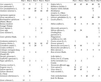
The germination experiment yielded 27 species among the 413 germinated seeds. Germinating seeds were found in 309 of the 640 core samples (48.3%). Twenty-six seedlings (6.3%) died prior to identification. Two individuals remained unidentified. Seed densities ranged from 618 to 3254 seeds m− 2 per plot, while species richness per plot ranged from 6 to 17 species. All important seed-bank characteristics are listed per plot in Table 1. A description of the seed-bank composition is given in full in Appendix 2.
Table 1 General seed-bank characteristics of the five investigated plots

Frequency: the number of samples containing germinated seeds; exclusive seed-bank species: species richness of species not recorded in the vegetation of the respective plot.
Spatial structure of the seed banks of individual species
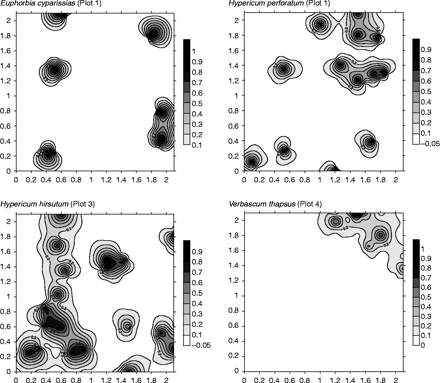
Modelled parameters of the experimental indicator-variograms can be found in Table 2. Eight species records were best fit by a pure nugget effect (not shown here), suggesting that their seeds are spatially distributed at random at the fine scale. However, nine species records could be modelled with either a spherical (2) or exponential (7) model. The nine species records showed medium to strong spatial dependence (RNE between 0.06 and 0.38; Table 2) at short distances, ranging from 10 to 35 cm. The average range over which spatial autocorrelation was recorded was 19.2 ( ± 8.1) cm. Visual representations of the spatial seed-bank structure of five species are shown in Fig. 1.
Table 2 Modelled parameters of the 17 estimated indicator-variograms

Frequency: the number of samples containing germinating seeds; IGF, indicative goodness of fit – the closer to zero the goodness of fit, the better the fit.

Figure 1 Contour maps visualizing the spatial distribution of different seed-bank species. Contour maps were constructed via indicator-kriging based on the parameters of the modelled indicator-variograms. Contours indicate the chance of finding a seed within the surface they delineate. Countour maps of the four remaining species that also showed spatial structure can be found in Appendix 3.
At least one species record per plot displays spatial structure, notwithstanding the large variation in plot seed-bank characteristics (Table 1). No species showed consistent spatial structure over all plots. At the same time, spatial structure seemed independent of species frequency (Table 2).
Discussion
Spatial structure of individual seed-bank species
In general, the result of initial dispersal is a clustered distribution of seeds centred more or less around the mother plant (Bigwood and Inouye, Reference Bigwood and Inouye1988). These mother plants are, in turn, spatially distributed (see, for example, Webster and Jenkins, Reference Webster and Jenkins2008), very often in a clustered pattern related to spatial variation in abiotic conditions and processes in the forest understorey (e.g. Lechowicz and Bell, Reference Lechowicz and Bell1991; Bengtson et al., Reference Bengtson, Falkengren-Grerup and Bengtsson2005). This will subsequently result in overlapping seed clusters of a plant species, both in space (via different individuals) and time (via the same individual). However, deposited seeds are far from immobile and can be displaced by ants, (burrowing) animals or wind (Vander Wall et al., Reference Vander Wall, Kuhn and Beck2005; Milcu et al., Reference Milcu, Schumacher and Scheu2006). In addition, as few species of persistent forest seed banks occur in the vegetation (Bossuyt and Hermy, Reference Bossuyt and Hermy2001), their seed clusters are subjected to disaggregative processes such as seed predation, failed germination and seed senescence, which slowly deplete the old seed clusters over time. Adding up the seed displacement by soil macrofauna, such as earthworms (Milcu et al., Reference Milcu, Schumacher and Scheu2006), the original fine-scale pattern is likely to be at least obscured or even destroyed. Nevertheless, even in this highly biologically active forest soil (mean pH H2O = 6.9), at least some of the fine-scale spatial structure ( < 2 m) remained intact, as nine species records could be modelled successfully using variograms (Table 2). Their spatial structure is both clustered, i.e. zones of high probability of seeds being present, and irregular, i.e. a random spatial distribution of the clusters (cf. Thompson, Reference Thompson1986; Bigwood and Inouye, Reference Bigwood and Inouye1988). However, our results also imply that the disaggregative effects of all previously mentioned processes on the spatial seed-bank structure may indeed erase the former, as in the remaining eight species records any initial spatial structure was likely obliterated.
Remarkably, no consistent trend in the presence or absence of spatial structure could be observed (cf. Thompson, Reference Thompson1986). Indeed, as most other species, even those species that were recorded many times over the different plots (i.e. Hypericum hirsutum, H. perforatum and Verbascum thapsus) were clustered at both low and high species frequencies. Hence, the presence or absence of spatial structure seemed to be independent of species frequency ( ≈ seed density).
The distance over which spatial autocorrelation was recorded (i.e. the range), was generally small (0.10–0.35 m) (Table 2), possibly suggesting limited seed dispersal. Indeed, despite their adaptations to disperse away from the mother plant, the species still seem to have brought a notable portion of their seeds into the soil locally (cf. Clark et al., Reference Clark, Poulsen, Bolker, Connor and Parker2005), likely near the former (sensu presently absent) mother plant. While these seeds could be considered as unsuccessful dispersers (Cousens et al., Reference Cousens, Wiegand and Taghizadeh2008), the seeds of persistent forest seed bank species do occupy a suitable habitat patch and consequently may have the highest probability of colonizing the site when suitable germination conditions arise. In the case of Verbascum thapsus, this has already been reported (Gross, Reference Gross1980). Hence, for persistent forest seed-bank species, this can be regarded a successful strategy to assure their survival, additional to the benefits of successful dispersal, particularly in the spatiotemporally highly heterogeneous forest environment (Runkle, Reference Runkle, Pickett and White1985). Combining both strategies, allows spatially distributed dormant species to enjoy a greater chance of encountering local disturbance.
Consequences of the small-scale spatial seed-bank patterns for sampling
The scarcity of information on small-scale spatial seed-bank patterns has resulted in a myriad of sampling designs (cf. Simpson et al., Reference Simpson, Leck, Parker, Leck, Parker and Simpson1989). The fine-scale seed-bank patterning this study visualized (Fig. 1) has significant relevance to future seed-bank sampling at similar scales, as the majority of seed-bank studies indeed sample the seed bank in 2 m × 2 m, 1 m × 1 m or even smaller (sub)plots. Next to a sufficiently large sampled volume or surface area – which is widely acknowledged to be of the utmost importance to obtain reasonably accurate seed-bank estimates (Thompson, Reference Thompson1986; Bigwood and Inouye, Reference Bigwood and Inouye1988) – we therefore argue that the sampling mode to gather these volumes should overcome the small-scale spatial seed-bank structure. One way to collect sufficiently large volumes within a plot, is to take few large samples rather than many small ones (Bigwood and Inouye, Reference Bigwood and Inouye1988). Many forest seed-bank studies (e.g. Sakai et al., Reference Sakai, Sato, Sakai, Kuramoto and Tabushi2005; Dassonville et al., Reference Dassonville, Herremans and Tanghe2006; Schelling and McCarthy, Reference Schelling and McCarthy2007) still sample forest seed banks in this way, likely due to practical and time limitations. Yet, the fine-scale patterns or clusters observed in our work (Fig. 1), may easily lead to biased estimates of all seed bank characteristics through ‘unfortunate’ plot placement (Bigwood and Inouye, Reference Bigwood and Inouye1988). Therefore, this study of small-scale seed-bank patterns corroborates the view that many small samples should be taken to achieve the pre-set volume or surface area (Bigwood and Inouye, Reference Bigwood and Inouye1988). However, the best way to collect these samples is by ensuring that their collection is independent (cf. Legendre, Reference Legendre1993), as they are likely to yield unbiased, precise plot seed-bank estimates. Linked to variograms, this means that core sampling needs to take place at a distance beyond the range, which defines the limit over which spatial dependence occurs (Webster and Oliver, Reference Webster and Oliver2007). However, it is difficult to formulate unequivocal advice on within-plot sampling distance, based on only nine ranges (Table 2). Nonetheless, most spatially structured species do have a small range, despite their large variation in plant traits. Therefore, we believe that within-plot sampling distances of 30–50 cm will likely suffice in most cases to return independent core samples, yielding unbiased and reasonably precise estimates of seed-bank composition and seed density.
Acknowledgements
J.P. thanks Josefien Delrue for fieldwork assistance, Glenn Matlack for suggestions on an earlier draft of the manuscript and two anonymous referees who helped to improve the manuscript.
Appendix 1
Vegetation description per seed-bank plot (2.1 m × 2.1 m). Vegetation composition per plot expressed as frequency of occurrence of individual species on 49 subplots (0.3 m × 0.3 m). Plant nomenclature follows Lambinon et al. (Reference Lambinon, De Langhe, Delvosalle and Duvigneaud1998)
Appendix 2
Seed-bank composition per seed-bank plot (2.1 m × 2.1 m) in terms of abundance (number of seeds/128 samples)/frequency (number of samples/128 samples) per species. Plant nomenclature follows Lambinon et al. (Reference Lambinon, De Langhe, Delvosalle and Duvigneaud1998)

Appendix 3
Contour maps visualizing the spatial distribution of the four remaining spatially structured seed-bank species. Contour maps were constructed via indicator-kriging based on the parameters of the modelled indicator-variograms. Contours indicate the chance to find a seed within the surface they delineate.