2. System design

2.1. Robot

The robot presented in this article is dumb-bell shaped with diameter 10 mm and length 12 mm (Fig. 1). The robot fabrication is accomplished using a 3D FDM printer. Due to the robot’s overall size, magnetic interaction is the most suitable actuation method. For this purpose, a hollow space is designed in the middle section of the robot for embedding a magnetic dipole. Thus, the robot’s location varies by generating an external magnetic field.

Figure 1. Robot’s configuration (a) the fabricated robot using FDM printer in a workspace with local and global coordinates. The hollow space within the robot is for embedding a permanent magnet disk where the magnetization is along the disk thickness (b) Robot’s drawing in mm.

In comparison to the default force-based pulling, using controlled torque leads to a rolling motion having a better resolution in displacement. The small resistance to motion in rolling compared to sliding or pulling leads to a more efficient motion. Pulling causes friction to resist the movement. However, friction helps rolling robots to move forward.

2.2. Magnetic force and torque

For an easier access, all the notations used in the paper are provided in Table I. An external magnetic field applies torque and force on a magnetic dipole, which can be calculated by:

(1) \begin{align}{\vec {\rm{F}}_{\rm{m}}} = \left( {{\rm{V}}\vec {\rm{M}}.\vec \nabla } \right)\vec {\rm{B}} \end{align}

(2) \begin{align}{\vec {\rm{T}}_{\rm{m}}} = {\rm{V}}\vec {\rm{M}} \times \vec {\rm{B}}\quad \end{align}

Where $\vec {F}_{m}$ and $\vec {T}_{m}$ are the acting force and torque on the magnetic body. $V$ , $\vec {B}$ , and $\vec {M}$ are the volume of magnetic dipole, the external magnetic field vector, and the magnetization vector, respectively. Based on (1), variation in a magnetic field generates a magnetic force. Therefore, the complexity of the control process reduces by generating a uniform magnetic field. Also, it is verified that torque-driven actuation scales better to miniature-sized robots [Reference Peyer, Zhang and Nelson41] and the uniform magnetic field can actuate our proposed robot effectively by applying external torque for rolling.

Table I. Parameters and variables which are used in the article.

2.3. Helmholtz coil

Several magnetic actuation systems for miniature robots are presented [Reference Yang and Zhang42]. As mentioned in Section 2.2, a uniform magnetic field generator is necessary to avoid applying force on the robot. To produce a uniform magnetic field, we designed a Helmholtz electromagnetic circular coil. The Helmholtz coil is constituted of two identical parallel coils (coaxial coils) where the separation distance between coils is equal to the radius of the coils. In this configuration, each pair carry equal current in the same direction. The magnetic field $B$ at the midpoint between the coils will be given by:

(3) \begin{align}{\rm{B}} = \frac{8}{{5\sqrt 5 }}{\frac{{\unicode{x03BC}_0}{\rm{NI}}}{\rm{R}}}\end{align}

Where $R$ is the radius of the coil, $N$ is the number of turns in each coil, $I$ is the current through the coils, and $\unicode{x03BC} _{0}$ is the magnetic permeability of free space. Creating a uniform magnetic field in the desired direction in 3D space is achievable by assembling three orthogonal Helmholtz pairs in three independent directions.

Enforcing some requirements in the design of Helmholtz coils facilitates the controlling process. These requirements are as follows:

1. 1. Each pair of Helmholtz coils must be able to generate at least 9mT.

2. 2. Each pair should be able to carry at least 5A current.

3. 3. The time constant of the coil should be less than the control loop period.

4. 4. The ripple of the currents should be minimized.

The second criterion defines the diameter of the wire, and the third and fourth specify the maximum and minimum value of self-inductance to wire resistance ratio, respectively. Also, increasing the frequency of PWM signals can be considered as a solution to the last requirement. Eventually, the remaining physical parameters can be evaluated by the first requirement. Taken all together, the following conditions should be satisfied:

\begin{align*}0.331{\rm{msec}} \ll {\frac{\rm{L}}{{\rm{R'}}}} \ll 20{\rm{msec}}\end{align*}

\begin{align*}{\rm{R'}} \lt 3.75\Omega \end{align*}

Where $L$ and $R'$ are the self-inductance and resistance of the coils, respectively.

The wire’s diameter, besides bobbin’s radius, height, width, and number of turns are design parameters. Hence, the relation between these parameters and the aforementioned requirements should be considered. Table II shows the parameters of the designed Helmholtz coil. Figure 2 depicts the fabricated Helmholtz coil assembly. The wire diameter is $1.30\,{\rm mm}$ .

Table II. Specifications of a three-pairs Helmholtz coil setup.

Figure 2. Fabricated Helmholtz Coil.

Since in each Helmholtz pair, the current of coils is identical, the coils of each pair are connected in series. The measured resistance and self-inductance of the system are shown in Table III. The comparison of theoretical and experimental values in Table III implies that the electrical specifications of the fabricated system are approximately the same as theory.

Table III. Measured self-inductance and resistance of three pairs.

Magnetic field uniformity plays an important role in the robot’s actuation. Therefore, the magnetic field at the midpoint along the axis of coil-pair for the smallest pair is experimentally measured. The normalized value of the magnetic field obtained by the theory and experiment is shown in Table IV, confirming the agreement between experiment and theory as well as uniformity of the magnetic field.

Table IV. Theoretical and experimental comparison of magnetic field uniformity in the smallest coil. The mean and standard deviation of errors for this comparison is equal to 0.0024 and 0.0057, respectively.

3. Dynamical equation

According to Eq. (2) given in section II, the difference between the robot magnetization dipole and the magnetic field direction induces torque on the robot. The free-body diagram of a 1DOF rolling robot is depicted in Fig. 3. In this figure $T_{m}$ , $mg$ , $f_{s}$ , and $N$ respectively stand for magnetic torque, weight, friction, and normal force exerted on the robot. With the assumption of no slipping, the dynamical equation of spinning caused by an external magnetic field can be written as follows:

(4) \begin{align}\mathrm{I}_{\mathrm{A}}\ddot{\unicode{x03B8} }+\mathrm{b}\dot{\unicode{x03B8} }=\mathrm{V}\!\left| \vec {\mathrm{M}}\right|\!\left| \vec {\mathrm{B}}\right| {sin } (\unicode{x03B1} -\unicode{x03B8} )\end{align}

Where $I_{A}$ is the robot’s moment of inertia around point A, $\theta$ is the robot’s spinning angle, $b$ is the damping term, and $\alpha$ is the angle of the magnetic field in the XZ plane. According to Eq. (4), the investigated robotic setup is a non-affine control system. It should be mentioned that the damping term has been added to mimic the experimental results.

The applied external magnetic field is close to the robot’s magnetization to avoid slipping. So the effort of the magnetic field can be simplified by $\alpha -\theta$ , which in turn can be expressed as follows:

(5) \begin{align}\mathrm{I}_{\mathrm{A}}\ddot{\unicode{x03B8} }+\mathrm{b}\dot{\unicode{x03B8} }=\mathrm{V}\!\left| \vec {\mathrm{M}}\right|\!\left| \vec {\mathrm{B}}\right| \left(\alpha -\theta \right)\end{align}

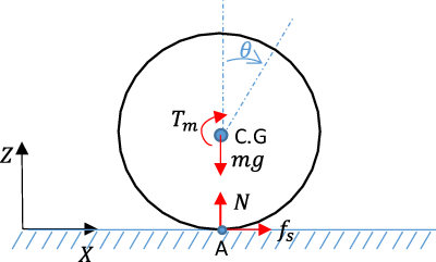
Figure 3. Schematic diagram of the force and torque on a rolling robot with constant heading.

In this case, the induced torque imposes a P controller to the dynamics of the system. By choosing an appropriate value for the robot’s specification and external magnetic field, the response of the system to an external magnetic field, has no overshoot and the settling time is less than time constant of the control loop. Thus, the physics of magnetic torque formulates a P controller, which has a stable response and can be regarded as a robust control to some extent. The robot’s moment of inertia can be omitted compared to the damping term, so we have:

(6) \begin{align}\mathrm{b}\dot{\unicode{x03B8} }=\mathrm{V}\!\left| \vec {\mathrm{M}}\right|\!\left| \vec {\mathrm{B}}\right| \left(\alpha -\theta \right)\end{align}

By dividing Eq. (6) by $\mathrm{V}\!\left| \vec {\mathrm{M}}\right|\!\left| \vec {\mathrm{B}}\right|$ and replacing $\frac{\mathrm{b}}{\mathrm{V}\!\left| \vec {\mathrm{M}}\right|\!\left| \vec {\mathrm{B}}\right| }$ by $\tau _{1}$ , we got:

(7) \begin{align}\unicode{x03C4} _{1}\dot{\unicode{x03B8} }+\unicode{x03B8} =\unicode{x03B1}\end{align}

By the same reasoning, the precession dynamics can be simplified as:

(8) \begin{align}\unicode{x03C4} _{2}\dot{\unicode{x03B3} }+\unicode{x03B3} =\unicode{x03B2}\end{align}

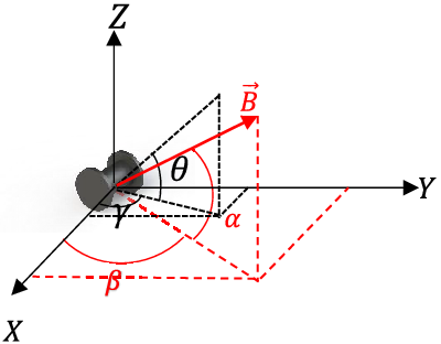
Where $\alpha$ is the magnetic field angle relative to XY plane (magnetic field spinning angle), $\beta$ is the angle between the projection of magnetic field in the XY plane with X axis (magnetic field heading angle), $\theta$ is the robot’s spinning angle, and $\gamma$ is the heading angle of the robot. These angles are shown in Fig. 4. Time constants $\tau _{1}$ and $\tau _{2}$ are in the order of a few milliseconds. Therefore, the response of system to magnetic field can be approximated by the solution of a first-order differential equation due to the low percentage of overshoot, which in turn can simulate the transient dynamics and the quasi-static manner of the movement.

This means if we can control the magnetic field direction effectively, then the robot’s heading and position can be controlled and synchronized with the external magnetic field.

The induced torque tries to align the robot dipole with the external magnetic field. Whenever these two vectors are aligned, the torque becomes zero, and the robot reaches a stable state. Based on Eq. (4), the stability, ripple, and settling time depend on the moment of inertia, the dipole moment, and the applied torque. According to the robot’s specifications, which are shown in Table V, it can be concluded that the robot dipole aligns with the external magnetic field very fast, that is less than the period of the control loop, and no fluctuation around the stable state can be seen.

Table V. Robot’s specification.

Figure 4. The direction of the magnetic field can be specified by angles $\alpha$ and $\beta$ , and the robot’s orientation can be specified by angles $\theta$ and $\gamma$ .

Generally, extracting the dynamical equation of a 2DOF robot having spinning and heading angle as state variables leads to some coupled terms. These coupled terms can be assumed as dynamics uncertainty which will be handled by the P controller of magnetic torque. Therefore, the bounded value of the coupled terms have no effects on the control process since the robot is always aligned with the external magnetic field.

the robot’s position can be expressed in polar coordinates (local coordinates in Fig. 1(a)) where the heading angle of the robot acts as the angular coordinate and the spinning angle which shift to displacement (by the rolling assumption) can be assumed as radial coordinate. This relations can also be converted to global coordinates that will be used for computing the error position.

4. Control algorithm

This research benefits from both neural network and fuzzy interpretation. This combination can simplify weight variation and antecedent classification [Reference Lin and Lee43]. A neuro-Fuzzy network, depicted in Fig. 5, consists of a fuzzy inference system implemented in the form of a neural network. Therefore, human experience can be employed to enhance the performance of the proposed network. Neuro-fuzzy networks consist of four layers, where each layer corresponds to different parts of the fuzzy rule. Layer one is associated with the real value of inputs. Layer two and three indicate fuzzification and antecedent parts of rules, respectively. In the last layer, the output of the network is evaluated by the use of Mamdani product inference engine and individual rule-based inference. Also, real values of rule’s consequent are defined as weights between layers three and four.

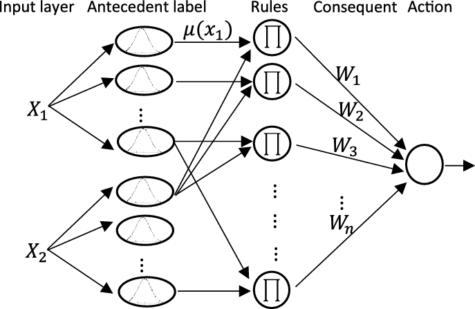
Figure 5. Neuro-fuzzy network.

Here, the fuzzy rules should be defined precisely for two reasons. First, because of the robot slipping, which will occur by higher torques and may lead to the loss of controllability. The robot and surface materials as well as the magnitude of applied torque are effective on the robot wheel slipping. The designed robot has two main motions; one motion is related to its heading change where its axis of spin changes. Another motion is related to its motion with fixed heading where the robot wheel spins. Based on the designed system, the robot heading changes with sliding of its wheel, but for accurate positioning of the robot, slipping must be avoided during spinning of the wheel. Based on the magnetic torque equation, magnetic field value and the difference between directions of magnetic field and the robot magnetic dipole, act as control inputs, so the other parameters must be chosen in the design procedure. The magnitude of the magnetic field and its direction should be properly controlled to steer the robot to the desired location without slipping. The other reason for precise fuzzy rules originates from the quick alignment of the robot’s dipole with the magnetic field direction, making it hard to compensate for errors. Hence, the weights of the network should be adjusted by a supervisor to have an accurate neural network. Usually, the supervisor contains a dataset which relates the input to the output. In this research, due to the simple nonlinear function between inputs and outputs, there is no need to generate a dataset, and Eq. (3) can be interpreted as a supervisor.

The robot’s position and heading is controlled by the external magnetic field. The closed-loop control system should calculate the coil currents to steer the robot to the desired position and heading. To control the robot’s position and heading, at first based on the position error, the desired heading and spinning angles $\gamma$ and $\theta$ are calculated. Then, according to Eqs. (7) and (8), the robot quickly aligns with the magnetic field’s direction that is suitable for controlling robot’s orientation. Therefore, the position control is converted to the angle control of the magnetization vector. Figure 6 depicts the block diagram of the feedback control system. To map angles $\alpha$ and $\beta$ of the magnetic field to the coils’ currents, the neuro-fuzzy network is developed. This network is tuned offline and applied in the closed-loop control system.

Figure 6. Controller algorithm (a) The block-diagram of the closed-loop control system (b) Further details of neuro-fuzzy controller.

According to the designed Helmholtz coil, the inputs of the system are currents of the three pairs, and outputs are magnetic field spinning and heading angles:

(9) \begin{align}\beta = {tan ^{ - 1}}\left( {{\frac{{{\rm{B}}_{\rm{y}}}}{{{\rm{B}}_{\rm{x}}}}}} \right)\qquad\quad \end{align}

(10) \begin{align}\alpha = {tan ^{ - 1}}\left( {{\frac{{{\rm{B}}_{\rm{z}}}}{\sqrt {{\rm{B}}_{\rm{x}}^2 + {\rm{B}}_{\rm{y}}^2} }}} \right)\end{align}

The neuro-fuzzy network needs to be an inverse function of the plant. Therefore, the inputs and outputs are reversed, compared to the system’s dynamics. The magnitude of the magnetic field vector needs to be more than 2mT to avoid fluctuations in the rotation. Fuzzy sets of inputs are constant, and they have Gaussian shape:

(11) \begin{align}\unicode{x03BC} = {{\rm{e}}^{{\dfrac{ - {{\left( {{\rm{x}} - {\rm{c}}} \right)}^2}}{{\sigma ^2}}}}}\end{align}

Where $x, c$ and $\sigma$ are input, center, and standard deviation of the membership function.

The neighboring membership functions should intersect with each other to have a continuous output. Thus, $\sigma$ is chosen 1.5 times the difference between centers of neighboring fuzzy sets. Each input has 7 fuzzy sets, which are distributed evenly on the input’s domain. Therefore, there are 49 rules in this network. The introduced error by the supervisor is as follows:

(12) \begin{align}{\rm{E}} = \frac{1}{2}{\left( {{{\rm{\alpha }}_{{\rm{In}}}} - {{\rm{\alpha }}_{{\rm{NF}}}}} \right)^2} + \frac{1}{2}{\left( {{{\rm{\beta }}_{{\rm{In}}}} - {{\rm{\beta }}_{{\rm{NF}}}}} \right)^2}\end{align}

Where the subscript $In$ and $NF$ indicate input and neuro-fuzzy output. According to the Eqs. (9) and (10), the weight variation is evaluated by gradient descent algorithm:

(13) \begin{align}\Delta \mathrm{W}_{\mathrm{i}}=-\unicode{x03B7} \left(\frac{\partial \mathrm{E}}{\partial \unicode{x03B1} _{\mathrm{NF}}}\left(\sum _{\mathrm{j}=\mathrm{x},\mathrm{y},\mathrm{z}}\frac{\partial \unicode{x03B1} _{\mathrm{NF}}}{\partial \mathrm{B}_{\mathrm{j}}}\frac{\partial \mathrm{B}_{\mathrm{j}}}{\partial \mathrm{I}_{\mathrm{j}}}\frac{\partial \mathrm{I}_{\mathrm{j}}}{\partial \mathrm{W}_{\mathrm{i}}}\right)+\frac{\partial \mathrm{E}}{\partial \unicode{x03B2} _{\mathrm{NF}}}\left(\sum _{\mathrm{j}=\mathrm{x},\mathrm{y},\mathrm{z}}\frac{\partial \unicode{x03B2} _{\mathrm{NF}}}{\partial \mathrm{B}_{\mathrm{j}}}\frac{\partial \mathrm{B}_{\mathrm{j}}}{\partial \mathrm{I}_{\mathrm{j}}}\frac{\partial \mathrm{I}_{\mathrm{j}}}{\partial \mathrm{W}_{\mathrm{i}}}\right)\right)\end{align}

Where $\eta$ is the learning rate, and $W_{i}$ is the weights of the neuro-fuzzy network. Variation in the sign of inputs does not change the absolute value of the output, so both inputs are restricted to the interval $\left[0,\frac{\pi }{2}\right]$ to reduce the nonlinearity of the system. Consequently, a simple rule can be applied to calculate the suitable currents for other quarters. Heuristic method can also be applied to the network to reduce the tuning time:

• • Rule 1: IF heading angle is along the X axis, Then the current of the medium pair ( $I_{y}$ ) is zero.

• • Rule 2: IF heading angle is along the Y axis, Then the current of the biggest pair ( $I_{x}$ ) is zero.

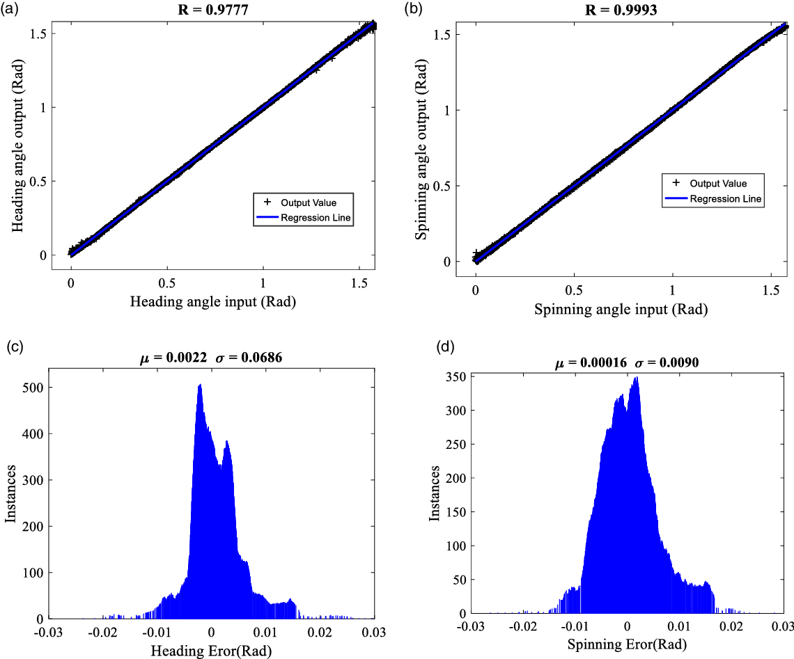
To this aim, 2000 random inputs were introduced to the system to train the network, and the weights are varied until the error reaches 1. In order to demonstrate the reliability of the network, several spinning and heading angles were introduced. Then, the spinning and heading angles were derived from the outputs of the network by the use of Eqs. (9) and (10).

The precision of training can be seen in Fig. 7. The Gaussian distribution of errors and the regression lines indicate a great match between the inputs and evaluated outputs.

Figure 7. Response of the neuro-fuzzy network. (a) Heading angle evaluated from the output of neuro-fuzzy network (3 pair currents) versus heading angle input. (b) spinning angle evaluated from the output of neuro-fuzzy network (3 pair currents) versus spinning angle input. (c) Gaussian distribution between heading input and evaluated heading output. (d) Gaussian distribution between spinning input and evaluated spinning output.

The mentioned neuro-Fuzzy controller is tuned offline, and its adequate performance is verified. For having an adaptive control, a critic can be added to the system to update neuro-Fuzzy weights in each step. This controller is called brain emotional learning based intelligent controller [Reference Lucas, Shahmirzadi and Sheikholeslami44], which has the ability to learn through the run time. The benefit of using a critic is that it does not need for observability of all states; therefore, this framework suits miniature magnetic robots.

5. Experiment

5.1. Setup specification

A camera with 20 FPS in 640 × 480 pixels is used to give the controller a snapshot as feedback, so The control loop frequency is limited by the camera’s capturing frequency which is 20 Hz. To have a real-time controller and perform high-speed image processing, we have used a PC. After calculation of the coils’ currents by the PC, these values are fed to an Arduino DUE; the Arduino board is used for converting these currents to duty cycle by:

(14) \begin{align}\unicode{x03C9} =46.52\sqrt {I}\end{align}

Where $\omega$ and $I$ are duty cycle and current, respectively. The above equation is determined based on the setup specifications and empirical tests in which the set voltage of the power source has been selected such that a current of 4.5 Amperes passes through the wires in the full duty cycle (steady current which can be passed through the wires without influencing the resistance’s value). This relation has been obtained under the assumption of low variation of the desired inputs to replace the dynamics of an RL circuit with a DC gain (extracting the effect of inductance). The Arduino sends PWM signals with the specific duty cycle to a high current motor driver (BTS7960 module). The inputs of this module are PWM signals and power source, which are initialized before each test. Afterwards, the output of the module is connected to the Helmholtz coil. Currents of the electromagnetic coils create a uniform magnetic field inside the workspace and the robot reorientation occurs. The frequency of PWM signals is chosen to be 10 kHz to avoid the ripple in currents. The block diagram of the components is shown in Fig. 8.

Figure 8. Hardware of closed-loop control system.

The linear power supply which is used in this study can provide 0 to 5 Amperes and the voltage can be varied from 0 to 30 volts. However by using a driver, the direction of current and voltage can be reversed to generate desired magnetic field. Also the resolution of power supply for current and voltage are 0.01 Amperes and 0.1 volts, respectively.

The coefficient of friction between substrate, made from acrylic glass and the robot, made from polylactic acid (PLA) is approximately 0.3. After several try and error, finally the magnetic field magnitude was set as 8 mT, and the difference between the external magnetic field and the robot dipole was adjusted to be 4 degrees in each step.

5.2. Results

A path was generated to set a desired track for the robot. This path was a straight line, which connected the current position of the robot to the destination. Due to the existence of uncertainty, the robot deviated from the generated path, so the robot’s heading ( $\gamma$ ) was corrected in each step. Figure 9 implies the error of the robot’s heading compared to the desired path. As can be seen, the error is negligible. The other angle which corresponds to the spinning angle ( $\theta$ ), will be increased or decreased based on the sign of the error near the desired point:

(15) \begin{align}\Delta {\rm{\alpha }} = {\rm{sign}}\left( {{\rm{r}} - {{\rm{r}}_{\rm{d}}}} \right) \times {\rm{C}}\!\left( {{{\rm{e}}_{\rm{R}}}} \right)\end{align}

Where $r$ and $r_{d}$ are the current and the desired position of the robot in a local coordinate where for any value of the robot heading, if the robot must move forward to reach its desired position, $sign(r-r_{d})$ becomes positive and vice versa. Parameter $C$ is a positive constant which depends on the error, and has two values, 0.01 or 0.03 depending on the distance between the desired and actual position of the robot, and the smaller value is used when the distance becomes smaller from a specific value. Also, a square window whose sides are 2 mm and centered around the desired point were introduced. Within this window, the robot’s position error is considered zero to avoid the variation in robot’s heading. The error window has a direct relation to the robot’s dimension. Therefore, this area can be decreased by a reduction in the robot’s size.

Figure 9. Regression line and the deviation of the robot in experiment in different magnitudes of the magnetic field.

The accuracy of positioning mainly depends on the generated magnetic field (actuator), control algorithm and camera (sensor). It is verified in section II that the external magnetic field is accurate enough to generate a homogenous field. Also Because of the small area of the workspace, the sensor’s sampling error can be neglected. Therefore, the main source of error is assigned to the controller algorithm. For this purpose, Figure 10 shows the worst-case scenario (by setting different set voltage) in the robot’s path which needs a sharp turn near the desired point. This turn can be ignored by variation in the weights of neural fuzzy network (Adaptive neural fuzzy network) and a predictor. Initially, the robot was at position $X=9.9\,{\rm cm}$ and $Y=5.6\,{\rm cm}$ . 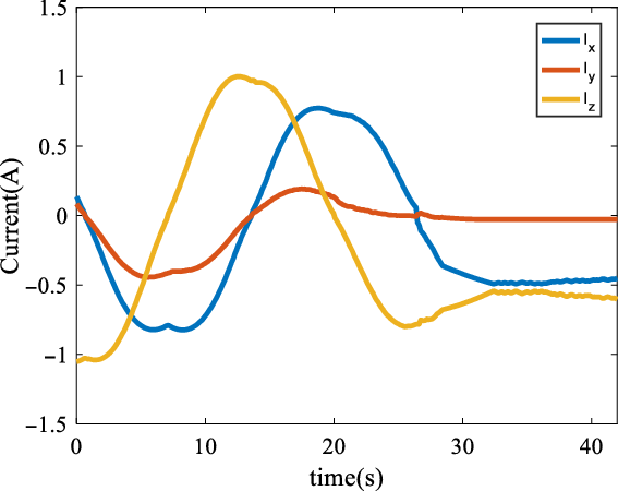The position’s error in response to $X_{d}=6$ cm and $Y_{d}=8$ cm. Also, the commanded currents for reaching the desired position are shown in Fig. 11. The position is captured by the camera and the robot was colored red so by using image processing techniques the position of the robot can be evaluated.

Figure 10. Position error and robot’s path in global coordinate.

Figure 11. Current of the coils in order to control the position of the robot.

Path controlling of the robot in a point to point manner was also investigated by the presented algorithm. In Fig. 12, the performance of the robot in response to half a sinusoidal wave is shown.

Figure 12. Robot’s point to point control in response to sinusoidal path.