


1. Introduction
The trajectory planning is a fundamental problem for manipulators used in many fields, and the goal of trajectory planning is to find a geometric path in Cartesian space or joint space with a given motion law; thus, the movement of manipulators is fast, accurate and stable while meeting obstacle constraints, kinematic constraints and dynamic constraints. Therefore, trajectory planning has important theoretical and engineering significance and has been deeply investigated by many researchers [Reference Chettibi1–Reference Abe3]. As Gasparetto points in [Reference Gasparetto, Boscariol, Lanzutti, Vidoni, Carbone and Gomez-Bravo4], to realize the trajectory planning for manipulators, a series of via-points of the end-effector are usually extracted in the Cartesian space firstly, and an inverse kinematic is employed to get the corresponding values of manipulator joints. Then, the complete trajectory in joint space is generated by interpolation function considering kinematic and dynamic limits of joints.
A trajectory planning method based on higher degree polynomials is proposed for serial-link manipulators in [Reference Boryga and Graboś5], in which the linear acceleration profiles of end-effector are planned as the polynomials of degrees 9, 7 and 5, and properties of the root multiplicity are used to construct the polynomial form. The numerical example results show that the polynomial with degree 7 performs better when considering only the trajectory without kinematic extremum value. But high-order polynomials have a problem that they are time-consuming to calculate. Ho and Cook use cubic and fourth-order spline to compose the trajectory, guaranteeing the continuity of position, velocity and acceleration [Reference Ho, Cook and Aleksander6]. However, the jerk will change suddenly at the via-points and eventually cause the unsmooth acceleration. The problem about the continuity of jerk is solved in [Reference Boscariol, Gasparetto and Vidoni7] using fourth-order and fifth-order polynomial functions and can also be settled by a polynomial trajectory method with an arbitrary degree [Reference Barghi Jond, Nabiyev and Çavdar8]. Besides, several papers use B-spline to compose trajectory, because B-spline has a good local support property, which means one of the via-points changes, the other parts of the trajectory will not be affected. Saramago et al. suggest the use of uniform cubic B-spline to solve the trajectory planning with kinematic constraints in [Reference Saramago and Junior9]. Quintic non-uniform B-spline is utilized in the process of joint interpolation, and the trajectory is optimized with iterative minimization procedure in [Reference Gasparetto and Zanotto10].
Although the trajectory of manipulators is already available using the methods mentioned above and satisfies kinematic constraints of joints, in the actual industrial manufacturing process, it is desirable that the manipulators have a short execution time, a small power consumption and other performance requirements. For those characteristics, many papers have proposed the minimum time, energy and jerk algorithm for trajectory planning. In [Reference Bobrow, Dubowsky and Gibson11,Reference Shin and McKay12], the minimum time of trajectory is realized through the position-velocity phase plane and dynamic programming techniques. Verscheure presents the optimized trajectory concerning the energy as well as time in [Reference Verscheure, Demeulenaere, Swevers, Schutter and Diehl13], which transforms the time-energy optimal problem into a convex control problem based on only one state variable. Besides, jerk also plays a notable role in the trajectory planning of manipulators. The high and discontinuous jerk will lead to vibration and a large joint impact that will affect the motion performance of manipulators. In this case, the fourth derivative of joint curves should be continuous [Reference Reiter and Müller14]. To guarantee the stability of robot movement, an objective function composed of total execution time and the integral of squared jerk along the trajectory is minimized in [Reference Gasparetto and Zanotto15]. Additionally, the method to search for a trade-off between the short execution time and sufficiently smooth trajectory is provided by [Reference Zanotto, Gasparetto, Lanzutti, Boscariol and Vidoni16]. Although the above researches optimize time-energy or time-jerk simultaneously, most of them use the weighting factors to combine two objective functions into one function, and those factors are usually hard to be determined except for multiple experiments.
To optimize the multi-objective functions at the same time rather than the functions combined by weighting factors, the multi-objective optimization methods are investigated. In this problem, there is no single optimal solution, while a set of optimal solutions that are equally valid that is known as the Pareto optimal set. Decision-makers can select a solution from the set according to the information provided by the criteria for evaluation. In these algorithms, the multi-objective evolutionary algorithm (MOEA) is now widely adopted. For example, Pires et al. [Reference Solteiro Pires, Tenreiro Machado and de Moura Oliveira17] propose a constrained multi-objective genetic algorithm to solve the trajectory problem with kinematic and dynamic constraints for a general motor-driven parallel kinematic manipulator. Huang et al. explore the elitist non-dominated sorting genetic algorithm method (NSGA-II) for two objectives, namely traveling time and mean jerk along the trajectory, and give the experiment results in [Reference Huang, Hu, Wu and Zeng18]. The application of multi-objective differential evolution (MODE) algorithm and NSGA-II algorithm in processing the trajectory optimization problem is investigated in [Reference Abu-Dakka, Valero, Suner and Mata19], and the results indicate that MODE technology converges faster than NSGA-II algorithm while the NSGA-II algorithm has a better Pareto optimal front. However, the MOEA is complicated and has too many parameters. Shi et al. propose a method based on quintic non-uniform rational B-spline to interpolate the joint trajectory, and NSGA-II is used to optimize the trajectory of manipulators under the three objectives: time, energy and jerk optimal. Finally, an average fuzzy membership function is adopted to select the potential optimal solution in Pareto front [Reference Shi, Fang and Guo20]. Other algorithms such as group heuristic algorithm are also used to solve the trajectory optimization problem. Chen et al. propose an improved immune clonal section algorithm to solve an optimization problem including three objective functions for a 6-UPU parallel platform, and the simulation results confirm the effectiveness of the method [Reference Chen, Li, Wang, Feng and Liu21]. Besides, an improved multi-objective ant lion algorithm is presented to solve the time-jerk-torque optimal problem for a six-axis robot [Reference Rout, Mahanta, Bbvl and Biswal22]. The multi-objective particle swarm optimization (MOPSO) algorithm is simple in principle with few parameters, and the particle information is saved and shared in different generations, thus its convergence is fast. In [Reference Huang, Liu, Yuan and Xu23], the MOPSO is used to optimize the motion trajectory of a space robot with dynamic disturbance; however, the multi-objective function is combined by weighting factors as mentioned above. Xu et al. use the MOPSO algorithm to optimize trajectory with three objectives including the optimal time, distance and energy in [Reference Xu, Li, Chen and Hou24] while the jerk is not considered and the evaluation criteria of Pareto front obtained by optimization algorithm is not provided.
As mentioned above, this paper proposed a trajectory planning method based on multi-objective optimization for manipulators in the presence of obstacles. Providing the initial, final points and several via-points, the initial trajectory is generated in joint space using quintic B-spline. The application of two virtual points ensures that the jerk of the both ends can be constrained to zero like the other kinematic parameters in the condition of the fifth-order curve. The objective functions include two criteria, namely as motion time and jerk impact defined as the integral of the squared jerk. The obstacle constraint is expressed as the minimum distance between the manipulator and obstacles and obtained by Gilbert–Johnson–Keerthi (GJK) algorithm. Introducing the degree of constraint violations, the Pareto domination is redefined. Then, constrained multi-objective particle swarm algorithm (CMOPSO) optimization algorithm is used to optimize the trajectory with minimum time and jerk. Finally, a membership function is proposed to select the best solution in the Pareto front obtained by the designed CMOPSO.
The rest of this paper is organized as follows. Section 2 provides the mathematical description of a standard manipulator and gives the optimization problem with constraints. The trajectory generation using quantic B-spline in joint space is established in Section 3. Section 4 proposes the CMOPSO algorithm to optimize the trajectory. Section 5 contains the simulation results and the corresponding analysis. Finally, the conclusion is drawn.
2. Problem statement
2.1. Mathematical model of the optimization problem
This section introduces the trajectory planning problem based on the PUMA560 manipulator, provides the objective functions of the trajectory optimization and redefines a dominance relationship by introducing the concept of constraint violation.
Unimation PUMA560 robot with six rotating joints is considered in this section, and its D-H parameters are exhibited in Table I. According to trajectory task, the PUMA robot should move from an initial point to the final point and pass through some specified via-points during the movement. The trajectory is usually defined in the task space, because the performance for task and obstacle avoidance is intuitively described, and many articles of the control field have been investigated in the operational space [Reference Souzanchi-K, Aliasghar, Mohammad-R and Fateh25,Reference Jalaeian-F, Fateh and Rahimiyan26]. Nevertheless, the trajectory planning problem is normally executed in the joint space with the advantage that the system could be easier to adjust the trajectory based on task requirements and constraints [Reference Gasparetto and Zanotto10]; in most cases, the via-points in Cartesian space will be converted into joint points through the kinematic inversion, suggesting that the trajectory planning is transferred from Cartesian space to joint space.
Table I. D-H parameters of PUMA560 robot.

The trajectory planning of the manipulator in this paper includes two part. The first step is that the manipulator moves from the initial points and passes through some via-points to a final point while the fourth derivate of each joint trajectory is continuous, and the positions, velocities, accelerations and jerks are subject to limitations. Second, the trajectory will be optimized to follow the time-jerk optimal and obstacle avoidance in joint space. It should be noticed that the two steps are applied simultaneously in the process of trajectory planning. Considering the execution time and global jerk in the movement, the optimization problem can be defined as
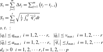 \begin{equation}\begin{array}{l} {S_{1} =\sum\limits_{j=1}^{m}\Delta t_{j} =\sum _{j=1}^{m}\left(t_{j} -t_{j-1} \right) } \\ \\[-9pt] {S_{2} =\sum\limits_{i=1}^{r}\sqrt{\frac{1}{T} \int _{0}^{T}\dddot{q}_{i}^{2} dt } } \\ \\[-9pt] {s.{\rm \; }t.{\rm \; \; \; }:} \\ \\[-9pt] {\left|q_{i} \right|\le q_{\max i} {\rm \; \; }i=1,2,\cdots r,{\rm \; \; }\left|\dot{q}_{i} \right|\le v_{\max i} {\rm \; \; \; }i=1,2,\cdots r} \\ \\[-9pt] {\left|\ddot{q}_{i} \right|\le a_{\max i} {\rm \; \; \; }i=1,2,\cdots r,{\rm \; }\left|\dddot{q}_{i} \right|\le j_{\max i} {\rm \; \; \; }i=1,2,\cdots r} \\ \\[-9pt] {d_{il} >0{\rm \; \; \; }i=1,2,\cdots r,l=1,2,\cdots p} \end{array}\end{equation}
where
 ${S_1}$
represents the time objective function;
${S_1}$
represents the time objective function;
 ${S_2}$
indicates the jerk objective function;
${S_2}$
indicates the jerk objective function;
 $\Delta {t_j}$
is the time interval between two consecutive via-points;
$\Delta {t_j}$
is the time interval between two consecutive via-points;
 ${q_i},{\dot q_i},{\ddot q_i}$
and
${q_i},{\dot q_i},{\ddot q_i}$
and
 ${\dot{\kern6pt}\ddot{\kern-4pt q}}_{i}$
are angle, velocity, acceleration and jerk of the
${\dot{\kern6pt}\ddot{\kern-4pt q}}_{i}$
are angle, velocity, acceleration and jerk of the
 $ith$
joint, respectively. Their corresponding boundaries are
$ith$
joint, respectively. Their corresponding boundaries are
 ${q_{\max i}},{v_{\max i}},{a_{\max i}}$
and
${q_{\max i}},{v_{\max i}},{a_{\max i}}$
and
 ${J_{\max i}}$
, respectively. Besides,
${J_{\max i}}$
, respectively. Besides,
 $T$
denotes the total traveling time; m and r are the number of via-points and manipulator joints, respectively.
$T$
denotes the total traveling time; m and r are the number of via-points and manipulator joints, respectively.
The collision constraint
 ${d_{il}}$
is defined by the minimum distance between the manipulator and obstacles. The collision constraint should remain
${d_{il}}$
is defined by the minimum distance between the manipulator and obstacles. The collision constraint should remain
 ${d_{il}}\,{\ge}\,0$
in the optimization process, suggesting that there is no collision in the generated trajectory. The calculation of
${d_{il}}\,{\ge}\,0$
in the optimization process, suggesting that there is no collision in the generated trajectory. The calculation of
 ${d_{il}}$
will be given in the following part. It should be noticed that time interval
${d_{il}}$
will be given in the following part. It should be noticed that time interval
 $\Delta {t_j}$
between two consecutive via-points is unknown and needs to be determined by optimization.
$\Delta {t_j}$
between two consecutive via-points is unknown and needs to be determined by optimization.
2.2. Constraint-containing Pareto dominance
In the single-objective optimization problem, there is only one optimal solution. It can be obtained by a simple and common mathematical method. However, in the multi-objective optimization problem, the mutual constraints of each objective function will make the performance improvement of one objective often at the cost of losing other performance. It is usually impossible to have a solution that optimizes the performance of all objective functions.
In terms of kinematic, the minimum time and the minimum jerk cannot be satisfied simultaneously. According to these objective functions, it can obtain a lot of solutions to form a non-inferior solution set, and it is difficult to judge the quality of those solutions. A suitable solution is hoped to be chosen from the set, and the solution should be guaranteed to be optimal. In [Reference Reyes-Sierra and Coello27], a method called Pareto dominance that is defined as follows is presented.
Definition 1: Given two vectors
 $\vec x$
,
$\vec x$
,
 $\vec y \in {R^m}$
, it can be defined that
$\vec y \in {R^m}$
, it can be defined that
 $\vec x \le \vec y$
if
$\vec x \le \vec y$
if
 ${x_i} \le {y_i}$
for
${x_i} \le {y_i}$
for
 $i=1,2, \cdots m$
, and that
$i=1,2, \cdots m$
, and that
 $\vec x$
dominates
$\vec x$
dominates
 $\vec y$
(denoted by
$\vec y$
(denoted by
 $\vec x \prec \vec y$
) if
$\vec x \prec \vec y$
) if
 $\vec x \le \vec y$
and
$\vec x \le \vec y$
and
 ${x_i} \ne {y_i}$
.
${x_i} \ne {y_i}$
.
Considering the kinematic constraints and the obstacle avoidance, the degree of constraint violation is introduced into the dominance relationship between the solutions. The constraint violation can be expressed as
 \begin{equation}cv\left( {\vec x} \right) = \sum\limits_{i=1}^N {\frac{{c{v_i}\left( {\vec x} \right)}}{{\max \left\{ {c{v_i}\left( {\vec x} \right)} \right\}}}} {\rm{ + }}\lambda \left( d \right)\end{equation}
where
 $c{v_i}\left( {\vec x} \right)$
is the
$c{v_i}\left( {\vec x} \right)$
is the
 $ith$
degree of constraint violation, and
$ith$
degree of constraint violation, and
 $\lambda $
is the penalty coefficient about the collision. If there is a collision in the optimization, namely
$\lambda $
is the penalty coefficient about the collision. If there is a collision in the optimization, namely
 $d \le 0$
,
$d \le 0$
,
 $\lambda $
will be a large number to increase the constraint violation, leading to an increase in the corresponding solution to be inferior. Meanwhile,
$\lambda $
will be a large number to increase the constraint violation, leading to an increase in the corresponding solution to be inferior. Meanwhile,
 $\lambda =0$
if the minimum distance
$\lambda =0$
if the minimum distance
 $d\,{>}\,0$
. The degree of constraint violation
$d\,{>}\,0$
. The degree of constraint violation
 $c{v_i}\left( {\vec x} \right)$
can be expressed as
$c{v_i}\left( {\vec x} \right)$
can be expressed as
 \begin{equation}c{v_i}\left( {\vec x} \right) = \left\{ \begin{array}{l}\max \left( {\left| {{h_i}\left( {\vec x} \right)} \right| - \varepsilon ,0} \right)\\ \\[-7pt] \max \left( {{g_i}\left( {\vec x} \right),0} \right)\end{array} \right.\end{equation}
where
 ${{{h}}_{{i}}}{\rm{\;}}$
and
${{{h}}_{{i}}}{\rm{\;}}$
and
 ${{{g}}_{{i}}}$
are equality and inequality constraints, respectively, and
${{{g}}_{{i}}}$
are equality and inequality constraints, respectively, and
 $\varepsilon \;$
is an acceptable threshold value. Based on the mentioned above, the Pareto domination can be rewritten as follows.
$\varepsilon \;$
is an acceptable threshold value. Based on the mentioned above, the Pareto domination can be rewritten as follows.
Definition 2: Given two vectors
 $\vec x,\vec y \in {R^m}$
, it can be said that
$\vec x,\vec y \in {R^m}$
, it can be said that
 $\vec x$
dominates
$\vec x$
dominates
 $\vec y$
if one of the following conditions is true: (1)
$\vec y$
if one of the following conditions is true: (1)
 $cv\left( {\vec y} \right) > cv\left( {\vec x} \right) \ge 0$
; (2)
$cv\left( {\vec y} \right) > cv\left( {\vec x} \right) \ge 0$
; (2)
 $cv\left( {\vec x} \right)=0,cv\left( {\vec y} \right)=0$
, and
$cv\left( {\vec x} \right)=0,cv\left( {\vec y} \right)=0$
, and
 $\vec x,\vec y$
meet Pareto dominance indicated as Definition 1.
$\vec x,\vec y$
meet Pareto dominance indicated as Definition 1.
The solutions can be judged by the redefined dominance and the ones that are not dominated will be added into Pareto front. It should be noted that some solutions in Pareto front may have a violation constraint
 $cv$
greater than 0, indicating that although those solutions are added into Pareto front, some of them may not satisfy all boundary constraints, and it should be considered in the selection of the optimal solution at last.
$cv$
greater than 0, indicating that although those solutions are added into Pareto front, some of them may not satisfy all boundary constraints, and it should be considered in the selection of the optimal solution at last.
3. Trajectory interpolation using B-spline
In this section, the quintic B-spline is used to obtain the formulation of the normalized motion profile along an axis of geometric path. The B-spline has good local support and convex hull characters and has been widely applied in robot trajectory planning. To ensure the jerk is smooth and continuous, the order of B-spline is given as 5. The
 $k$
order B-spline can be defined recursively by means of the De Boor formula [Reference De Boor28] as
$k$
order B-spline can be defined recursively by means of the De Boor formula [Reference De Boor28] as
 \begin{equation}p(u) = \sum\limits_{i=0}^n {{d_i}} {N_{i,k}}(u)\end{equation}
where
 $p(u)$
is the joint point,
$p(u)$
is the joint point,
 ${d_i}$
is the control point of B-spline, u is a vector consisting of non-decreasing normalized knots and
${d_i}$
is the control point of B-spline, u is a vector consisting of non-decreasing normalized knots and
 ${N_{i,k}}$
denotes the basis function of B-spline that can be expressed as
${N_{i,k}}$
denotes the basis function of B-spline that can be expressed as
 \begin{equation}\left\{ \begin{array}{l}{N_{i,0}}(u) = \left\{ \begin{array}{l}1\qquad {\rm{ }}{u_i} \le u \le {u_{i+1}}\\ \\[-7pt] 0\qquad {\rm{ others}}\end{array} \right.\\ \\[-7pt] {N_{i,k}}(u) = \dfrac{{u - {u_i}}}{{{u_{i + k}} - {u_i}}}{N_{i,k - 1}}(u) + \dfrac{{{u_{i + k+1}} - u}}{{{u_{i + k+1}} - {u_{i+1}}}}{N_{i+1,k - 1}}(u){\rm{ }}\end{array} \right.\end{equation}
where
 ${u_i}$
(i = 0, 1, ···, m = n + k+1) defines a sequence of knots necessary. This recursive formula suggests that it needs
${u_i}$
(i = 0, 1, ···, m = n + k+1) defines a sequence of knots necessary. This recursive formula suggests that it needs
 ${u_i},{u_{i + k+1}}$
, total normalized
${u_i},{u_{i + k+1}}$
, total normalized
 $k+2$
knots to determine the basis function
$k+2$
knots to determine the basis function
 ${N_{i,k}}$
and the joint point defined in the region
${N_{i,k}}$
and the joint point defined in the region
 $u \in \left[ {{u_i},{u_{i+1}}} \right]$
is at most related to
$u \in \left[ {{u_i},{u_{i+1}}} \right]$
is at most related to
 $k+1$
control points, and is not subject to others.
$k+1$
control points, and is not subject to others.
The
 $r$
degree derivative of the B-spline curve can be calculated according to the following recursive formula:
$r$
degree derivative of the B-spline curve can be calculated according to the following recursive formula:
 \begin{equation}{p^r}(u) = \sum\limits_i^{n - r} {d_i^r} {N_{i,k - r}}(u){\rm{ }}\end{equation}
where
 ${{d}}_{{{\;i\;}}}^{{{\;r}}}\left( {{{\;i=0,\;1,\;n}} - {{r}} + {\rm{1}}} \right)$
is the control point of
${{d}}_{{{\;i\;}}}^{{{\;r}}}\left( {{{\;i=0,\;1,\;n}} - {{r}} + {\rm{1}}} \right)$
is the control point of
 ${\rm{rth}}$
derivative of
${\rm{rth}}$
derivative of
 $p(u)$
and can be expressed as
$p(u)$
and can be expressed as
 \begin{equation}d_j^i = \left\{ \begin{array}{l@{\quad}l}{d_j} & i=0\\ \\[-7pt] \left( {k+1 - i} \right)\dfrac{{d_j^{i - 1} - d_{j - 1}^{i - 1}}}{{{u_{j + k+1 - i}} - {u_j}}}& i=1,2, \cdots r\end{array} \right.\end{equation}
To keep a continuous trajectory in terms of jerk, the order of B-spline should be equal to 5, and the values at knots vector extremities should have multiplicity
 $k+1$
so that the control points connect the initial and final points. These characteristics lead to the results that, given a sequence including
$k+1$
so that the control points connect the initial and final points. These characteristics lead to the results that, given a sequence including
 $f$
via-points in the joint space, the number of control points
$f$
via-points in the joint space, the number of control points
 $n+1 = k + f - 1$
, and the number of knots
$n+1 = k + f - 1$
, and the number of knots
 $m+1=2k + f+1$
. To improve numerical accuracy in floating-point arithmetic computation [Reference Grandine and Klein29], the knots vector is normalized and can be expressed as
$m+1=2k + f+1$
. To improve numerical accuracy in floating-point arithmetic computation [Reference Grandine and Klein29], the knots vector is normalized and can be expressed as
 \begin{equation}\mathbf{\textbf{u}} = \left[ {0,0, \cdots 0,{u_{k+1}}, \cdots {u_{f + k - 2}},1,1, \cdots 1} \right]\end{equation}
The other knots
 ${u_{k+1}}, \cdots {u_{f{\rm{ + }}k - 2}}$
are obtained by normalizing the time sequence as
${u_{k+1}}, \cdots {u_{f{\rm{ + }}k - 2}}$
are obtained by normalizing the time sequence as
 \begin{equation}{u_i} = {u_{i - 1}} + \frac{{\left| {\Delta {t_{i - k - 1}}} \right|}}{{\sum\limits_{j=0}^{n - 1} {\left| {\Delta {t_j}} \right|} }},i = k+1,k+2, \cdots ,f + k - 2\end{equation}
Since the via-points sequence includes two virtual points at the second and the last-second positions, the jerk could be constrained to 0 at both ends in the condition of 5 order. In this case, only
 $f - 2$
constraint equations can be obtained by (4), and
$f - 2$
constraint equations can be obtained by (4), and
 $k+1$
constraint equations provided by boundary conditions are needed to solve the control points vector
$k+1$
constraint equations provided by boundary conditions are needed to solve the control points vector
 ${\bf{d}}$
. The boundary conditions can be expressed by the constraints of velocity, acceleration and jerk at both ends, which can be written as
${\bf{d}}$
. The boundary conditions can be expressed by the constraints of velocity, acceleration and jerk at both ends, which can be written as
 \begin{equation}\begin{array}{l}v\left( t \right) = \sum\limits_{i=0}^{n - 1} {c_v^i} {N_{i,k - 1}}\left( t \right)\\ \\[-7pt] a\left( t \right) = \sum\limits_{i=0}^{n - 2} {c_a^i} {N_{i,k - 2}}\left( t \right)\\ \\[-7pt] j\left( t \right) = \sum\limits_{i=0}^{n - 3} {c_j^i} {N_{i,k - 3}}\left( t \right)\end{array}\end{equation}
The parameters
 $c_v^i,c_a^i,c_j^i$
in (10) can be expressed as.
$c_v^i,c_a^i,c_j^i$
in (10) can be expressed as.
 \begin{equation}\begin{array}{l}c_v^i = \dfrac{k}{{{u_{i + k+1}} - {u_{i{\rm{ + }}1}}}}\left( {{d_{i+1}} - {d_i}} \right)\!,\quad i=0,1, \ldots ,n\\ \\[-7pt] c_a^i = \dfrac{{k - 1}}{{{u_{i + k}} - {u_{i+1}}}}\left( {c_v^{i{\rm{ + }}1} - c_v^i} \right)\!,\quad i=0,1, \ldots ,n - 1\\ \\[-7pt] c_j^i = \dfrac{{k - 2}}{{{u_{i + k - 1}} - {u_{i+1}}}}\left( {c_a^{i{\rm{ + }}1} - c_a^i} \right)\!,\quad i=0,1, \ldots ,n - 2\end{array}\end{equation}
For simplicity, define the symbol
 $N = n+1$
,
$N = n+1$
,
 $F = f - 2$
. According to the
$F = f - 2$
. According to the
 $F$
equations provided by (4) and the
$F$
equations provided by (4) and the
 $k+1$
supplementary equations provided by (10), the expression used to solve the control points can be written as the following formula (12). It could be noted that
$k+1$
supplementary equations provided by (10), the expression used to solve the control points can be written as the following formula (12). It could be noted that
 ${v_0},{v_f},{a_0},{a_f},{j_0},{j_j}$
are the kinematic constraints at both ends mentioned above.
${v_0},{v_f},{a_0},{a_f},{j_0},{j_j}$
are the kinematic constraints at both ends mentioned above.
 \begin{equation}{\mathbf{d}}={{\mathbf{Q}}^{ - 1}}{\mathbf{p}}\end{equation}
where
 \begin{equation*}{\textbf{d}} = {\left[ {{d_0},{d_1}, \cdots {d_n}} \right]^T} \in {R^{N \times 1}},{\textbf{p}} = {\left[ {{p_1},{p_2}, \cdots {p_{f - 2}},{v_0},{v_f},{a_0},{a_f},{j_0},{j_f}} \right]^T} \in {R^{N \times 1}},{\bf{Q}} = \left[ \begin{array}{l}{Q_1}\\{Q_2}\end{array} \right] \in {R^{N \times N}}\end{equation*}
 \begin{equation*}{{\bf{Q}}_1} = {\left[ \begin{array}{c@{\quad}c@{\quad}c@{\quad}c}1&&&\\ \\[-7pt]{N_{1,k}}\left( {{u_{k+2}}} \right)&{N_{2,k}}\left( {{u_{k+2}}} \right)& \cdots &{N_{n,k}}\left( {{u_{k+2}}} \right)\\ \\[-7pt]{N_{1,k}}\left( {{u_{k+3}}} \right)&{N_{2,k}}\left( {{u_{k+3}}} \right)& \cdots &{N_{n,k}}\left( {{u_{k+3}}} \right)\\ \\[-7pt] \vdots & \vdots & \vdots & \vdots \\ \\[-7pt] {N_{1,k}}\left( {{u_{k + f - 1}}} \right)& {N_{2,k}}\left( {{u_{k + f - 1}}} \right) & \cdots &{N_{n,k}}\left( {{u_{k + f - 1}}} \right)\\ \\[-7pt] &&&1\end{array} \right]_{F \times N}}\!,\end{equation*}
 \begin{equation*}{{\bf{Q}}_2} = {\left[ \begin{array}{c@{\quad}c@{\quad}c@{\quad}c@{\quad}c@{\quad}c@{\quad}c}{b_{1,1}}&{b_{1,2}} &&&&&\\ \\[-7pt]{b_{2,1}}&{b_{2,2}}&{b_{2,3}}&&&{\rm{ 0 }}&\\ \\[-7pt]{b_{3,1}}&{b_{3,2}}&{b_{3,3}}&{b_{3,4}}&&&\\ \\[-7pt]&&&&&{b_{1,n - 1}}&{b_{1,n}}\\ \\[-7pt]&{\rm{ 0 }}&&&{b_{2,n - 2}}&{b_{2,n - 1}}&{b_{2,n}}\\ \\[-7pt]&&&{b_{3,n - 3}}&{b_{3,n - 2}}&{b_{3,n - 1}}&{b_{3,n}}\end{array} \right]_{6 \times N}}{\rm{ }}\end{equation*}
The boundary conditions of the initial and final via-points can be expressed only by control points
 ${\bf{d}}$
through the recursive formula (10), and
${\bf{d}}$
through the recursive formula (10), and
 ${b_{r,i}}(i=1,2, \cdots r+1{\rm{ and }}\ i = n - r, \cdots n)$
is the coefficient before each control point of those conditions. Thus, given a sequence of via-points and corresponding time, the trajectory can be defined by (4) and (12). Furthermore, the velocity, acceleration and jerk of the trajectory can also be determined through the above recursive formula (10).
${b_{r,i}}(i=1,2, \cdots r+1{\rm{ and }}\ i = n - r, \cdots n)$
is the coefficient before each control point of those conditions. Thus, given a sequence of via-points and corresponding time, the trajectory can be defined by (4) and (12). Furthermore, the velocity, acceleration and jerk of the trajectory can also be determined through the above recursive formula (10).
4. Multi-objective optimization for the trajectory
In this section, the CMOPSO is used to optimize the trajectory generated by quintic B-spline, enabling the end-effector would follow the given via-points and satisfy the kinematics constraints and obstacle avoidance. The schematic of the whole optimization process is depicted in Fig. 1

Figure 1. The schematic of manipulator trajectory planning.
4.1. Obstacle avoidance constraints
GJK method is an iterative algorithm that supports the collision detection and calculation of the minimum distance between any convex shapes and has fast convergence speed. It should be noticed that the obstacles in this paper are all simple geometric shapes since the GJK algorithm is only valid for convex bodies. In practical applications, simple enveloping surfaces are often used to surround obstacles with complex shapes to simplify the calculation process. Moreover, each link of manipulator has an assumption to be circumscribed by the rectangular prism. In this way, eight points can be used to represent each link, and the coordinates of each point relative to the world coordinates can be obtained by
 \begin{equation}{P_{ij}} = \left[ \begin{array}{l}{{\bf{R}}_{\bf{j}}},{\rm{ }}{{\bf{t}}_{\bf{j}}}\\ \\[-7pt] {\bf{0}}{\rm{ }},{\rm{ }}1\end{array} \right]{P_i}{\rm{ }}\left( {i=1,2 \ldots 6,j=1,2 \ldots 8} \right)\end{equation}
where
 ${P_i},{P_{ij}}$
are the origin coordinates of each link and the coordinates of the corresponding eight rectangular vertexes, respectively; matrices
${P_i},{P_{ij}}$
are the origin coordinates of each link and the coordinates of the corresponding eight rectangular vertexes, respectively; matrices
 ${{\bf{R}}_{\bf{j}}}$
and
${{\bf{R}}_{\bf{j}}}$
and
 ${{\bf{t}}_{\bf{j}}}$
represent the rotation matrix and translation matrix, respectively. Let a set
${{\bf{t}}_{\bf{j}}}$
represent the rotation matrix and translation matrix, respectively. Let a set
 ${d_{il}}$
defines the minimum distance between the
${d_{il}}$
defines the minimum distance between the
 $ith$
link and
$ith$
link and
 $lth$
obstacle, and the collision distance
$lth$
obstacle, and the collision distance
 $d$
is defined as
$d$
is defined as
 \begin{equation}d = \min \left( {{d_{11}},{d_{12}}, \ldots {d_{il}}} \right)\end{equation}
During the motion of the manipulator, the collision distance
 $d$
needs to be calculated at each time t. A joint configuration would be obtained in each step of the optimization. Then, the coordinates of the end-effector in Cartesian coordinates can be calculated using forward kinematics, and the collision distance
$d$
needs to be calculated at each time t. A joint configuration would be obtained in each step of the optimization. Then, the coordinates of the end-effector in Cartesian coordinates can be calculated using forward kinematics, and the collision distance
 $d$
would be solved by GJK algorithm and (14). If the distance satisfies
$d$
would be solved by GJK algorithm and (14). If the distance satisfies
 $d\,{>}\,0$
under the current joint configuration, it indicates that the configuration is acceptable, otherwise it needs to be rejected.
$d\,{>}\,0$
under the current joint configuration, it indicates that the configuration is acceptable, otherwise it needs to be rejected.
4.2. Constrained multi-objective particle swarm algorithm
The MOPSO algorithm is proposed by Coello et al. [Reference Coello, Pulido and Lechuga30] and has been widely used to solve multi-objective problems because of its high speed of convergence and simplicity [Reference Bastos-Filho and Miranda31]. The MOPSO algorithm introduces the concept of external archive to store non-dominated solutions in iteration process; selecting the global best particle in the archive can motivate the convergence of the algorithm. Furthermore, the objective space is divided into hypercubes to calculate the coordinates of each non-dominated solution and the number of solutions contained in each hypercube. Table II presents the symbol explanations in the optimization algorithm.
Table II. Nomenclature used in MOPSO algorithm.

The first step of MOPSO procedure is to initialize the particle population with
 $N$
,
$N$
,
 $VEL$
and
$VEL$
and
 $POP$
. The position of each particle is a random value within the upper and lower boundary. Then, the fitness value
$POP$
. The position of each particle is a random value within the upper and lower boundary. Then, the fitness value
 ${\rm{Cost}}$
and constraint violation
${\rm{Cost}}$
and constraint violation
 $cv$
of each particle can be calculated according to (1) and (3).
$cv$
of each particle can be calculated according to (1) and (3).
Using the constraint-containing Pareto dominance described in definition 2, non-dominated particles are stored in archive
 $REP$
, and the location of those particles can be determined by adaptive grid method.
$REP$
, and the location of those particles can be determined by adaptive grid method.
In the main loop of MOPSO algorithm,
 $gBest$
is selected from
$gBest$
is selected from
 $REP$
based on the distribution density of particles and Roulette Wheel Selection method [Reference Goldberg and Deb32] firstly. Furthermore, the speed and position of each particle can be calculated using the equations proposed in [Reference Coello, Pulido and Lechuga30]. However, the constant inertia factor
$REP$
based on the distribution density of particles and Roulette Wheel Selection method [Reference Goldberg and Deb32] firstly. Furthermore, the speed and position of each particle can be calculated using the equations proposed in [Reference Coello, Pulido and Lechuga30]. However, the constant inertia factor
 $\omega $
is modified to sigmoid inertia factor as
$\omega $
is modified to sigmoid inertia factor as
 \begin{equation}\omega ={1\mathord{\left/ {\vphantom {1 \left(1{\rm +}\exp \left(\frac{\left(c_{1} {\rm +}c_{2} \right)iter}{\max \_ iter} -c_{2} \right)\right)}} \right.} \left(1{\rm +}\exp \left(\frac{\left(c_{1} {\rm +}c_{2} \right)iter}{\max \_ iter} -c_{2} \right)\right)}\end{equation}
where
 ${c_1},{c_2}$
are the adjustment coefficients, and those factors depend on the values of inertia factor at the initial and final positions that will be given in the algorithm. Besides,
${c_1},{c_2}$
are the adjustment coefficients, and those factors depend on the values of inertia factor at the initial and final positions that will be given in the algorithm. Besides,
 $iter$
is the current generation. It should be noted that the first generation
$iter$
is the current generation. It should be noted that the first generation
 $iter$
is considered to be 0. A small inertia factor is suitable for particle swarm to search in a small range while a large factor is suitable for large-scale search. The sigmoid function guarantees that the
$iter$
is considered to be 0. A small inertia factor is suitable for particle swarm to search in a small range while a large factor is suitable for large-scale search. The sigmoid function guarantees that the
 $\omega $
value decreases as the number of iterations increases, and the changing process is smooth. After performing a boundary check on the particles, all of them are ensured within the boundaries.
$\omega $
value decreases as the number of iterations increases, and the changing process is smooth. After performing a boundary check on the particles, all of them are ensured within the boundaries.
The next operations are the same with initialization, such as calculating fitness, determining non-dominated solution and updating the
 $REP$
. To prevent the particle population from converging so rapidly that it could converge to the local optimum in global optimization, a mutation operator is applied with a certain probability that it changes with the number of iterations. The flowchart of MOPSO is illustrated in Fig. 2.
$REP$
. To prevent the particle population from converging so rapidly that it could converge to the local optimum in global optimization, a mutation operator is applied with a certain probability that it changes with the number of iterations. The flowchart of MOPSO is illustrated in Fig. 2.

Figure 2. The flow chart of multi-objective particle swarm optimization.
4.3. Performance indicators for MOPSO
MOPSO algorithm or other multi-objective optimization algorithms offer an approximate Pareto front, and it is necessary to evaluate this front. The distribution and uniformity of the optimal set are two crucial performance indicators. The spacing (SP) indicator and
 $\Delta $
index [Reference Ali, Siarry and Pant33] are used to evaluate uniformity and generality of the solution set distribution. The SP indicator is computed with (16)
$\Delta $
index [Reference Ali, Siarry and Pant33] are used to evaluate uniformity and generality of the solution set distribution. The SP indicator is computed with (16)
 \begin{equation}SP(S) = \sqrt {\frac{1}{{\left| S \right| - 1}}\sum\limits_{i=1}^{\left| S \right|} {{{\left( {\bar d - {d_i}} \right)}^2}}}\end{equation}
where
 ${d_i}$
is the distance between a point and the closest point in the Pareto front approximation,
${d_i}$
is the distance between a point and the closest point in the Pareto front approximation,
 $\bar d$
is the mean value of
$\bar d$
is the mean value of
 ${d_i}$
and
${d_i}$
and
 $\left| S \right|$
is the number of the points in the Pareto front. The small value of SP means that the Pareto front obtained is evenly distributed.
$\left| S \right|$
is the number of the points in the Pareto front. The small value of SP means that the Pareto front obtained is evenly distributed.
Another indicator
 $\Delta $
index is written as
$\Delta $
index is written as
 \begin{equation}\Delta = \frac{{{d_f} + {d_l} + \sum\limits_{i=1}^{\left| S \right| - 1} {\left| {{d_i} - \bar d} \right|} }}{{{d_f} + {d_l} + \left( {\left| S \right| - 1} \right)\bar d}}\end{equation}
where
 ${d_f}$
and
${d_f}$
and
 ${d_l}$
are the Euclidean distances between the extreme solution of one objective and the boundary solutions of the Pareto front approximation. The other notations remain the same meaning as before. The small value of
${d_l}$
are the Euclidean distances between the extreme solution of one objective and the boundary solutions of the Pareto front approximation. The other notations remain the same meaning as before. The small value of
 $\Delta $
indicates that the Pareto front is distributed widely.
$\Delta $
indicates that the Pareto front is distributed widely.
MOPSO algorithm provides a Pareto front including many non-dominated solutions, and decision-makers should select an optimal solution according to a criterion. The fuzzy membership function is an effective method combining the fitness value of the objective function. A linear membership function is presented in [Reference Saramago and Junior9] and the membership value is obtained by average method.
In this paper, the Z-type function is utilized to evaluate the membership value, and the function is exhibited in Fig. 3 and (18). It is expected that particles close to the optimal value will be more considered, suggesting that they have a large membership value while particles far from the optimal value are considered as little as possible.
 \begin{equation}{u_i}(j) = \left\{ \begin{array}{l@{\quad}l}1&{f_i}(j) \le f_i^a\\ \\[-7pt]1 - 2{\left( {\frac{{{f_i}(j) - f_i^a}}{{f_i^b - f_i^a}}} \right)^2}& f_i^a \le {f_i}(j) \le \frac{{f_i^a + f_i^b}}{2}\\ \\[-7pt]2{\left( {\frac{{{f_i}(j) - f_i^b}}{{f_i^b - f_i^a}}} \right)^2}&\frac{{f_i^a + f_i^b}}{2} \le {f_i}(j) \le f_i^b\\ \\[-7pt]0& {f_i}(j) \ge f_i^b\end{array} \right.\end{equation}
where
 ${f_i}(j)$
is the value of the objective function
${f_i}(j)$
is the value of the objective function
 $\left( {i=1,2} \right)$
with a non-dominated solution from
$\left( {i=1,2} \right)$
with a non-dominated solution from
 $REP$
;
$REP$
;
 $f_i^a,f_i^b$
are the threshold values of the objective function. The membership value is defined as 1 in the threshold range of the optimal value, otherwise is 0. The fuzzy membership value is defined as
$f_i^a,f_i^b$
are the threshold values of the objective function. The membership value is defined as 1 in the threshold range of the optimal value, otherwise is 0. The fuzzy membership value is defined as
 \begin{equation}u\left(j\right)={\left(u_{1} \left(j\right)+u_{2} \left(j\right)\right)\mathord{\left/ {\vphantom {\left(u_{1} \left(j\right)+u_{2} \left(j\right)\right) \max \left\{u_{1} \left(j\right)+u_{2} \left(j\right)\right\}}} \right.} \max \left\{u_{1} \left(j\right)+u_{2} \left(j\right)\right\}}\end{equation}

Figure 3. Fuzzy membership function.
Firstly, the membership value of each particle is calculated using (16); then, the solutions whose constraint violation
 $cv=0$
will be considered, as mentioned above. The one with the largest fuzzy membership value is selected as the global optimal solution.
$cv=0$
will be considered, as mentioned above. The one with the largest fuzzy membership value is selected as the global optimal solution.
5. Test comparison and discussion
In this section, the proposed method is tested in two cases, one of which is compared with other methods without obstacles, and another is verified in the presence of simple obstacles.
5.1. Comparative test without obstacles
The via-points of each joint are listed in Table III, and these data are also used in [Reference Gasparetto and Zanotto10], which will be compared in the next. Each joint has two virtual via-points, and the kinematic constraints are provided in Table IV. The MOPSO algorithm parameters are set as: swarm size is 100, repository size is 100, maximum iteration is 50, the number of grids per objective is 7, mutation probability is 0.2, leader selection pressure is 2 and the sigmoid inertia factor
 ${c_1}=2\ln 3,{c_2} = - \ln \left( {2/3} \right)$
. Substituting
${c_1}=2\ln 3,{c_2} = - \ln \left( {2/3} \right)$
. Substituting
 ${c_1}$
and
${c_1}$
and
 ${c_2}$
into (13), the initial and final inertia factor can be calculated as 0.6 and 0.1, respectively. The velocity, acceleration and jerk of the initial and final via-point of the B-spline are set to 0. The vector of the time interval
${c_2}$
into (13), the initial and final inertia factor can be calculated as 0.6 and 0.1, respectively. The velocity, acceleration and jerk of the initial and final via-point of the B-spline are set to 0. The vector of the time interval
 $\Delta {t_j}$
between two consecutive via-points is the optimization variable. The total running time of the constrained MOPSO algorithm is about 43.286 seconds.
$\Delta {t_j}$
between two consecutive via-points is the optimization variable. The total running time of the constrained MOPSO algorithm is about 43.286 seconds.
Table III. Via-point of each joint.

Table IV. Kinematic constraints of the manipulator.

The simulation results are illustrated from Figs. 4–10. The Pareto front obtained by the CMOPSO algorithm is presented in Fig. 4. According to the Pareto optimal solution set, the objective time ranges from 8.722 s to 15.072 s, and the jerk indicator ranges from
 $29.26{\rm{^\circ /}}{{\rm{s}}^3}$
to
$29.26{\rm{^\circ /}}{{\rm{s}}^3}$
to
 $153.41{\rm{^\circ /}}{{\rm{s}}^3}$
. The shortest execution time corresponds to the largest jerk index, and vice versa. The overall trend is that a decrease in one objective value is accompanied by an increase in another. The constraint violation of all solutions in the Pareto front is 0.
$153.41{\rm{^\circ /}}{{\rm{s}}^3}$
. The shortest execution time corresponds to the largest jerk index, and vice versa. The overall trend is that a decrease in one objective value is accompanied by an increase in another. The constraint violation of all solutions in the Pareto front is 0.

Figure 4. Pareto front of time-jerk optimization.
Figure 5 illustrates the fuzzy membership values of all solutions in the front, which can help decision-makers select the global optimal solution. It could be observed that the 51st solution has the maximum membership value of 1 in the Pareto front. To some extent, the solution closer to the extremum solution at both ends has a smaller fuzzy membership value. The SP indicator describes the uniformity of the solution set distribution, and it measures the standard deviation of minimum distance from each solution to others. The SP value is obtained as 1.0854 using the method mentioned above, while the ideal value is 0. Figure 6 exhibits the distance relative to the mean value between
 $ith$
solution and
$ith$
solution and
 $\left( {i+1} \right)th$
solution using the ratio equation
$\left( {i+1} \right)th$
solution using the ratio equation
 $\left( {{d_i} - \bar d} \right)/\bar d$
. It could be noted that some values have a big difference with the average.
$\left( {{d_i} - \bar d} \right)/\bar d$
. It could be noted that some values have a big difference with the average.

Figure 5. Fuzzy membership value of each solution in Pareto front.

Figure 6. Relative distance of each particle in the Pareto front.
Another measure indicator is the index that measures the extent of the solution set obtained, and its value is 0.8927. In Saravanan’s works [Reference Saravanan, Ramabalan and Balamurugan34], the index is 0.80147 and 0.9854 using the NSGA-II and MODE method, respectively.
Taking the minimum traveling time from Pareto optimal solution, the time intervals optimized by the proposed trajectory planning method mentioned above are provided in Table V. Figures 7–10 illustrate the angle, velocity, acceleration and jerk of each joint with the minimum traveling time of 8.722s. Due to the boundary constraints, the velocity and acceleration of the first and final points are set to 0 while the jerk is also guaranteed to be 0 using the virtual points. The jerk curve in Fig. 10 is continuous, guaranteeing the smoothness of the trajectory.
Table V. Time intervals optimized by MOPSO.


Figure 7. Joints angle with a minimum time of 8.722 s.

Figure 8. Joints velocity with a minimum time of 8.722 s.

Figure 9. Joints acceleration with a minimum time of 8.722 s.

Figure 10. Joints jerk with a minimum time of 8.722 s.
Table VI illustrates the maximum kinematic values including velocity, acceleration and jerk of each joint obtained by the proposed method, and those values are compared with Gasparetto’s work [Reference Gasparetto and Zanotto10] that uses B-spline and Sequential Quadratic Programming method to optimize the trajectory. It can be revealed that the maximum velocity and acceleration optimized by this paper are a little larger than those given in [Reference Gasparetto and Zanotto10], while the jerk is the opposite. Table VII offers the mean kinematic values of each joint that are compared with the above work. In this case, the values are well comparable with those provided in [Reference Gasparetto and Zanotto10] concerning the mean velocity and acceleration, and the mean values of jerk obtained by the proposed method are lower than those in [Reference Gasparetto and Zanotto10]. As Gasparetto pointed out in [Reference Gasparetto, Boscariol, Lanzutti, Vidoni, Carbone and Gomez-Bravo4], a small value of jerk can reduce the excitation of resonance frequencies and suppress stress for actuators. The difference is caused by the fact that the control points of B-spline are used to express the kinematic constraints rather than the real kinematic values in [Reference Gasparetto and Zanotto10]. This can effectively reduce the complexity of calculation but will result in the numerical differences. The comparison indicates that the proposed method can also provide a comparative solution.
Table VI. Maximum kinematic values of each joint by the optimization algorithm.

Table VII. Mean kinematic values of each joint by the optimization algorithm

5.2. Test with obstacles
The test for three cases with different numbers of obstacles is illustrated in Fig. 11. Due to the fact that the GJK algorithm can only be applied to convex hull, the obstacles in the test are simple geometric shapes or assemblies of them. The trajectory of the manipulator end-effector in Cartesian space is shown in Fig. 11(a)–(c). Under the constraint conditions, the manipulator follows the optimal trajectory and avoids collision. In case (c), the manipulator moves from an initial joint point to the final joint point (120°, 60°, 60°, 100°, 40°, 90°), passing through via-points while avoiding collision with three obstacles. It can be obtained that the objective function about motion time ranges from 9.233 s to 19.460 s while the function of the jerk ranges from
 $13.868{\rm{^\circ /}}{{\rm{s}}^3}$
to
$13.868{\rm{^\circ /}}{{\rm{s}}^3}$
to
 $126.250{\rm{^\circ /}}{{\rm{s}}^3}$
.
$126.250{\rm{^\circ /}}{{\rm{s}}^3}$
.

Figure 11. Trajectory of the manipulator end-effector with different obstacles.
The decomposed trajectory of the x-axis, y-axis and z-axis is illustrated in Fig. 12. Kinematics of each joint are exhibited in Figures 13–16. The velocity, acceleration and jerk at both ends of the trajectory are constrained to zero, and the curves are smooth and continuous.

Figure 12. Decomposed trajectory of three arises with case (c).

Figure 13. Angle of each joint in the obstacle test (c).

Figure 14. Velocity of each joint in the obstacle test (c).

Figure 15. Acceleration of each joint in the obstacle test (c).

Figure 16. Jerk of each joint in the obstacle test(c).
It should be noted that the trajectory planning is conducted in joint space, so the motion actually performed by the end-effector and manipulator links is not easily predictable due to the nonlinear mapping from joint space to Cartesian space, indicating that the trajectory planning using the proposed method should be applied in the case of few and simple obstacles, otherwise the trajectory would have a probability of not being able to cross the obstacles.
6. Conclusion
This paper presents a trajectory planning method based on multi-objective optimization for manipulators in the presence of obstacles. Motion time and joint jerk are used to compose the multi-objective functions. Quintic non-uniform B-spline with virtual points is employed to generate trajectory in joint space according to the given via-points.
GJK algorithm is adopted to calculate the minimum distance between the manipulator and obstacles. The constraints including obstacle avoidance and kinematics constraints are solved by the introduced degree of constraints violation, and it is utilized to redefine Pareto dominance. Combining the redefined dominance, CMOPSO algorithm with a sigmoid inertia factor is adopted to optimize the time interval in B-spline. Then, the Pareto front is measured by SP indicator and
 $\Delta $
index, and a fuzzy membership value based on the proposed Z-type function is adopted to evaluate the solutions with the purpose of selecting the global best solution in the front.
$\Delta $
index, and a fuzzy membership value based on the proposed Z-type function is adopted to evaluate the solutions with the purpose of selecting the global best solution in the front.
Finally, the proposed method is tested in two cases, and the results demonstrate the effectiveness of this method in performing an optimal trajectory planning for manipulators.
Funding
This paper is supported by the Project supported by the National Natural Science Foundation of China (item number: 11672184).
Conflicts of Interest
No conflict of interest exits in the submission of this manuscript, and manuscript is approved by all authors for publication.
Availability of Data and Material
All data generated or analyzed during this study are included in this article.


