1. Introduction
The leakage of hazardous substances including chemicals, biological products, and radioactive materials may cause serious consequences such as exploding and poisoning. It is vital to identify the emission sources to provide early warning and treatment. Therefore, it is important to investigate the source tracing methods with high accuracy and efficiency. The process of source tracing is constrained by the following factors: First of all, the source tracing is greatly affected by the complex atmospheric conditions. Second, there may be many leakage sources whose locations are uncertain. Third, it is impossible to recognize the gas diffusion path with human eye and due to that it is always invisible. Finally, the manual method by portable sensors will cost too much time in source tracing. Moreover, it may be unsafe for the operators in some cases.
The source tracing methods can be divided into two types: identification algorithms based on static sensors and tracing algorithms based on mobile sensors. Several algorithms based on static sensor networks and inverse dispersion algorithms have been discussed by Hutchinson [Reference Hutchinson, Oh and Chen1]. For source identification with static sensors, the inversion algorithm is combined with the gas concentration distributions, terrain, and atmospheric conditions. In this method, the leakage source parameters are estimated by solving the inverse dispersion problem. Different algorithms including optimization and statistic approximations models have been proposed to estimate the source term with static sensors. Haupt et al. have utilized genetic algorithms to estimate the source parameters [Reference Haupt2]. Ma et al. combined classic optimization method with heuristic method to estimate the source parameters [Reference Ma, Gao, Zhang and Wang3,Reference Ma, Deng and Zhang4]. Hazarta and Kopka et al. used the Markov Chain Monte Carlo (MCMC) method to provide samples for Bayesian inference to reconstruct the source parameters [Reference Hazart, Giovannelli, Dubost and Chatellier5,Reference Kopka, Wawrzynczak and Borysiewicz6]. Ma and Wang et al. have used particle swarm optimization (PSO) method and statistic approximation method to identify the leakage source parameters [Reference Wang, Chen, Qiu, Ma, Zhu, Wang and Qiu7–Reference Flesch, Wilson and Harper10]. Flesch et al. proposed a method based on inverse Lagrangian Stochastic (LS) dispersion model to predict the gas dispersion and estimate the source parameters.11 However, the source tracing methods with static sensor networks have some disadvantages such as insufficient sensing area, poor mobility, high cost, and complex algorithm.
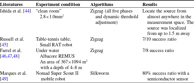
Table I. Some experimental results of other authors.

The mobile tracing methods are based on mobile sensors. Bionic source tracing algorithm is one of the typical methods to trace the emission source with a mobile sensor. Bionic algorithms simulate the behavior of natural creatures to search and locate the source of odor. Kowaldo and Lilienthal et al. have summarized some source tracing methods inspired by the behaviors of the living bodies to trace the odors, [Reference Kowadlo and Russell12–Reference Ishida, Hayashi, Takakusaki, Nakamoto, Moriizumi and Kanzaki16] such as moths Escherichia coli bacteria using, lobsters, blue crabs. This kind of bionic algorithm is called chemotaxis algorithm, which is guided by the gas concentration gradient during the source tracing [Reference Russell, Bab-Hadiashar, Shepherd and Wallace17–Reference Lytridis, Virk, Rebour and Kadar19]. Based on the principle of chemotaxis, Lytridis and Pasternak et al., proposed Silkworm, BRW (biased random walk), and levy-taxis algorithm for large-scale turbulent scenarios [Reference Lytridis, Virk, Rebour and Kadar19,Reference Pasternak, Bartumeus and Grasso20]. Another kind of bionic source tracing algorithm is chemotaxis algorithm, which combines the wind field with chemical concentration to find the location of the leak source. Among them, Zigzag or Dung Beetle is a typical algorithm coupling the anemotaxis and chemotaxis, where the sensor moves in a Zigzag form to find the boundary of the gas plume and then return, back and forth [Reference Ishida, Kagawa, Nakamoto and Moriizumi21]. Plume-centered search algorithm was designed to move continually toward the center of the plume, while tracing upwind [Reference Dusenbery22–Reference Rodriguez, Ramirez and De Pieri24]. Step-by-step algorithm makes a movement in the direction between the concentration gradient and upwind direction [Reference Kuwana and Nagasawa25,Reference Pyk, Badia, Bernardet, Knusel, Carlsson, Gu, Chanie, Hansson, Pearce and Verschure26]. The advantages of chemotaxis and an emotaxis algorithm are that the cost functions of them are just a two-valued form; the route planning is just determined by the wind direction or the concentration gradient or both of them; the absolute values of the concentration are not necessary. In spite of this, limited information may not provide enough detail about the source, which has an impact on location accuracy. Table I shows the comparison results of different chemotaxis and anemotaxis algorithms from other authors, and a detailed summary of different algorithms have made by Russell et al [Reference Kowadlo and Russell12]. However, it is difficult to compare the results from different researches quantitatively and accurately due to that the experimental conditions for different researches were varied as shown in Table I.
Moreover, another kind of bionic source tracing algorithm, Fluxotaxis algorithm, was proposed by Zarzhitsky et al. Fluxotaxis algorithm combines the measurements of fluid, chemical concentrations, and the estimation of mass flux to estimate the source of leakage [Reference Zarzhitsky, Spears, Spears and Thayer27]. In recent years, the tracing algorithms based on the model and information-driven process, which predicts the next movement with the forward model and acquired information, were presented [Reference Hernandez Bennetts, Lilienthal, Neumann and Trincavelli28,Reference Farrell, Li, Pang, Arrieta and Ieee33,Reference Pang and Farrell34]. In this kind of algorithm, the search strategies are guided by complex algorithms, such as Bayesian theory, optimization approximation, hidden Markov model, particle filter, naïve reasoning machine, entrotaxis-jump, and so on [Reference Hernandez Bennetts, Lilienthal, Neumann and Trincavelli28–Reference Zhao, Chen, Zhu, Chen, Wang and Ma35]. Hernandez et al. utilized Kernel DM+V algorithm and the variance maps to approximate the source parameters [Reference Hernandez Bennetts, Lilienthal, Neumann and Trincavelli28]. Yu et al. designed a source tracing algorithm by coupling the zigzag search strategy and an evolutionary gradient algorithm [Reference Yu, Cheng, Wang, Shang, Peng and Zhu29]. Kowadlo et al. used Bayesian inference to construct the multi-hypothesis tree to search for the sources [Reference Kowadlo and Russell30]. Pang and Farrell designed a random algorithm based on Bayesian inference to build a plume model during the source tracing process. They viewed the source tracing process as a problem of optimizing dynamic functions and the optimized value was the location of the source [Reference Farrell, Li, Pang, Arrieta and Ieee33,Reference Pang and Farrell34]. Vergassola and Kowadlo et al. proposed the Infotaxis algorithm, which can estimate the probability distribution map of the source based on the concentration measured by the robot, and then the robot’s next moving direction was calculated with Bayesian probability [Reference Hutchinson, Oh and Chen36,Reference Vergassola, Villermaux and Shraiman37]. Moraud and Martinez verified the effectiveness of the algorithm in an indoor artificial wind farm environment [Reference Moraud and Martinez38]. On the other hand, some researchers proposed a robot combined with machine vision and olfactory sensors to trace the source, as well as robot swarm work coordinately to trace the source [Reference Subchan, White, Tsourdos, Shanmugavel and Żbikowski39–Reference Yeon, Visvanathan, Mamduh, Kamarudin, Kamarudin and Zakaria41]. Because more information about concentration and environment were utilized and more complex algorithms were designed for routine planning, the location accuracy would be improved with Fluxotaxis and model-driven algorithms than that with chemotaxis and anemotaxis algorithms. In spite of this, the requirement of accurate absolute concentration and atmospheric parameters such as atmospheric stability and speed makes it more complex and the efficiency would be lost with long time computation.
Although different source tracing algorithms with mobile sensors have been proposed as discussed above, there are still some limitations for these researches. First, the quantitative evaluation and comparison of different source tracing algorithms with experiments have not been found in current researches. Further, the searching space in outdoors is still limited in reported researches. Hence, it is significant to investigate the accuracy and efficiency of different mobile source tracing algorithms with experiments. Another issue for unknown source identification is that it is important to identify the unknown compositions accurately during the source tracing. However, common metal–oxide–semiconductor (MOS) gas sensors equipped on the robot have cross-response for different gases. Thus, a gas sensor is inevitably affected by other gas substances during the tracing.
In this research, a mobile source tracing robot was designed and different typical bionic source tracing algorithms including Silkworm and Zigzag algorithm was tested in the open-air environment. A new source tracing algorithm, zigzag–Silkworm algorithm, combing the two algorithms was proposed and verified in outdoor experiments. Then, an artificial olfactory system (AOS) based on sensor array and machine learning model was designed to improve the recognition ability for unknown gas compositions during the tracing. Further, the principles and performances of different algorithms were compared in this research. Finally, the mobile sensor with AOS were verified and compared with different algorithms with experimental data.
2. Experimental Setup
2.1. The structure of mobile source tracing robot system
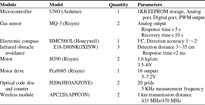
The structure of the source tracing robot system is shown in Fig. 1. The robot detected the gas concentration in the atmosphere and it communicates with the remote monitoring system by an APC220 wireless antenna (APPCON). The robot was equipped with gas sensors (MQ-3, Risym), obstacle avoidance modules (E18-D80NK, JXINW), electronic compass (HMC5883L, Honeywell), and other sets. The main parameters of the robot are shown in Table II.
Table II. Details of mobile source tracing robot.

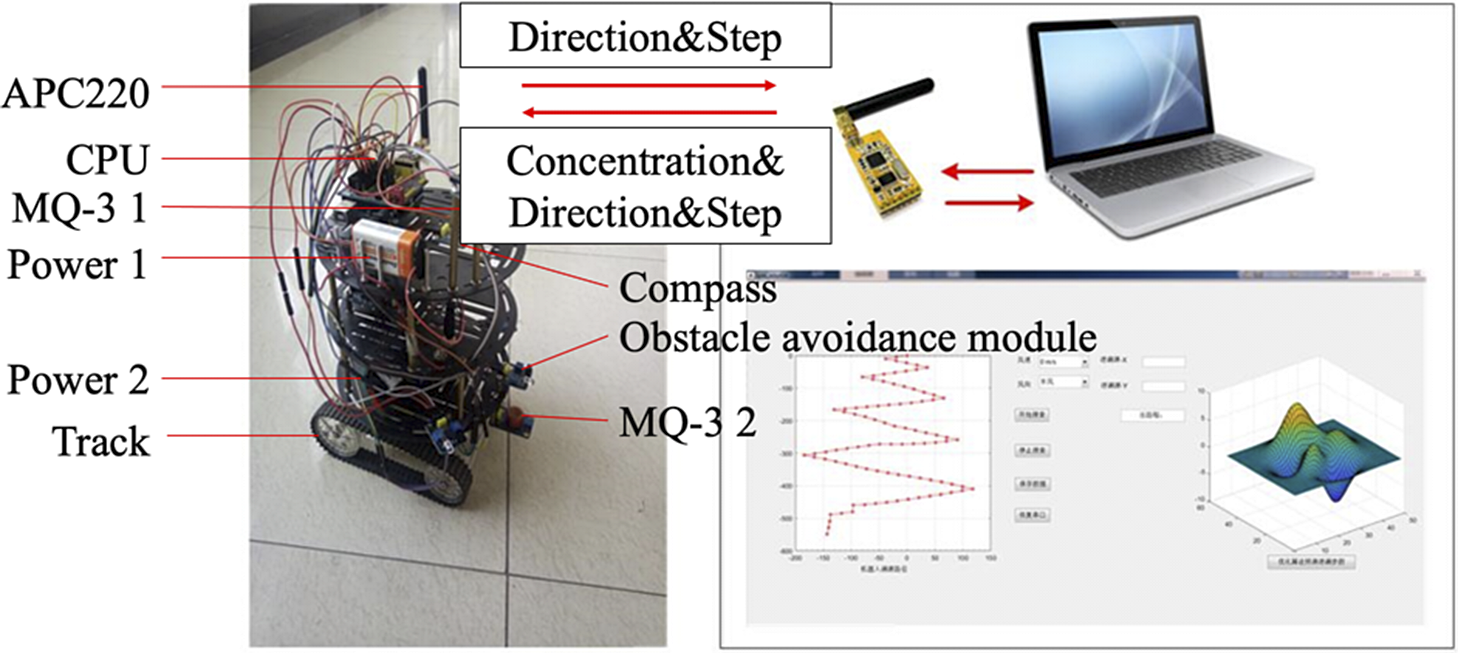
Figure 1. The structure of the mobile source tracing system.
The gas sensor, MQ-3 ethanol is based on the QM-NG1 probe and the PT1301 boost chip to capture the emission gases in the experiment. The gas-sensitive material of MQ-3 is tin dioxide (SnO2), which has low conductivity in clean air. The sensor can respond and recover within 5 s at different concentrations. It takes about 8 s for the robot to measure the concentration and complete the next rotation, thus it has enough time to respond and recover during the tracing. In addition, the robot was equipped with two sensors on the top and bottom, and the average value over multiple time periods based on two sensors were adopted to evaluate the plume, which may reduce the response errors from certain one sensor during the moving.
2.2. The experiment conditions
-
(1) The experiment site: An open-air site in the campus of Xi’an Jiaotong University was selected as the experiment site. The field is flat with an area of 10 by 20 m.
-
(2) The atmosphere conditions: Based on the long-time monitoring of wind direction and speed, the direction of the prevailing wind was north and west. In the season of our experiments, the wind speed was always less than 4 m·s–1 and the atmospheric conditions were stable during the night time of 20:00–23:00.
-
(3) The simulation of the leakage: A high-pressure fog generator with a maximum release rate of 0.5 L/min was used to release the volatile substances to simulate the leakage in the source tracing experiments. The ethanol was mixed with water with the ratio of 1:4 to be the emission materials. The emission rate can be controlled by the generator. As shown in Fig. 2, the experiments were carried out in the outdoor environment with a relatively stable atmospheric condition.
3. The Principles of Bionic Algorithms
3.1. Principle of Silkworm algorithm
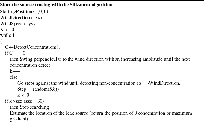
Silkworm algorithm imitates the process of male silkworm moth to trace the pheromone released from female moth. First, the moth swings in the crosswind direction with increasing steps. When the gas plume is detected, it moves one step toward the upwind direction, and then continues to swing in the crosswind direction with increasing amplitude. If no valid gas concentration is detected after set cycles, it is judged to arrive at the vicinity of the emission source and the search process is terminated. The flow of the Silkworm algorithm is shown in Fig. 3. The pseudocode of Silkworm algorithm is shown in Table III.
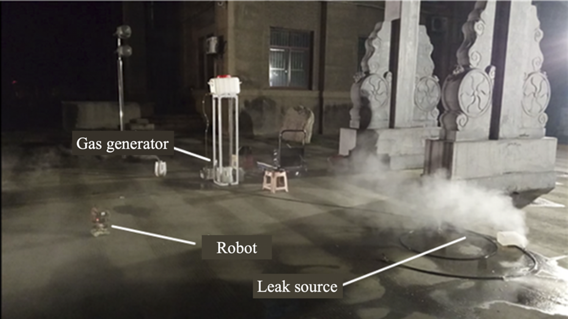
Figure 2. The site of source tracing experiment.
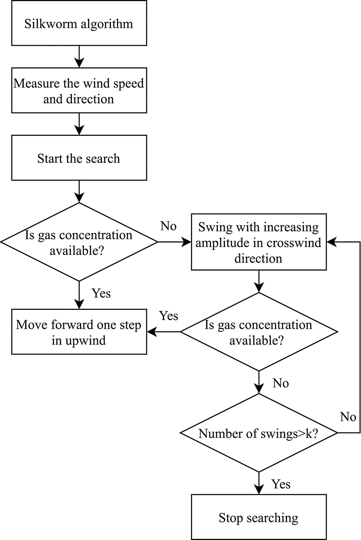
Figure 3. The flow chart of Silkworm algorithm.
3.2. Principle of Zigzag algorithm
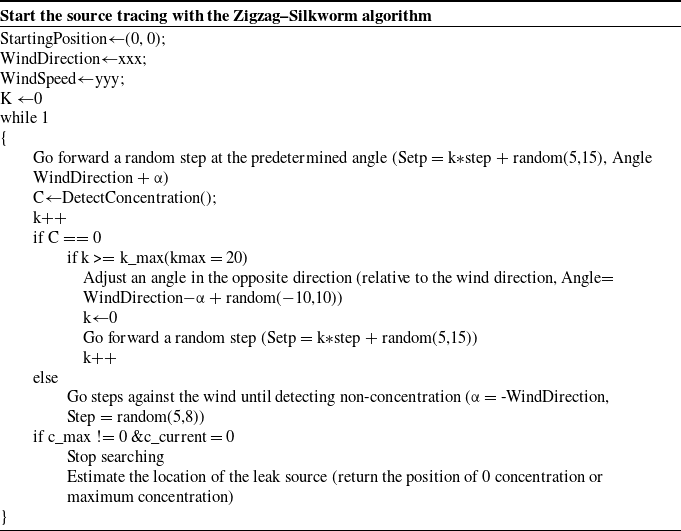
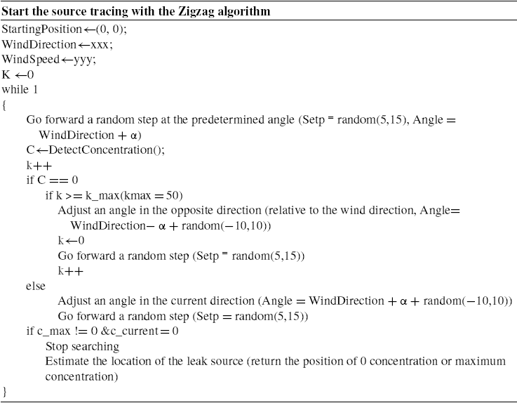
The Zigzag algorithm is inspired by the foraging process of Dung beetles [Reference Ishida, Nakamoto, Moriizumi, Kikas and Janata15]. The principle of the Zigzag tracing algorithm is to find the boundaries of the gas plume and then go back to a certain angle. The robot moves forward in the form of zigzag between the boundaries of the plume. The flow chart of the Zigzag algorithm is shown in Fig. 4. Table IV lists the pseudocode of Zigzag algorithm.
3.3. Principle of zigzag–Silkworm algorithm
According to the principle of Silkworm and Zigzag algorithms, they have some inherent limitations. First, the swept area with the Silkworm during the searching process is small, and the robot swings continuously in crosswind direction until stopping if it is unable to detect the concentrations. Second, there may be cases that the boundary of the plume could not be found due to the continuous variation of the atmosphere in the source tracing with Zigzag algorithm.
Table III. Pseudocode of Silkworm algorithm.

To trade-off the advantages and disadvantages of Silkworm and Zigzag algorithms, an improved algorithm, is proposed. It combines the stepping and swing search strategy of the Silkworm and the retrace search strategy of the Zigzag, thus it is called zigzag–Silkworm algorithm. The source tracing process of zigzag–Silkworm is similar to that of Silkworm, but the vertical swing is at an angle of 30°–60° along the upwind while it is 90° in the Silkworm. The robot will swing in a form of zigzag with a gradually increasing amplitude at a certain angle in the upwind direction if no valid gas concentration is detected in the early stage of the zigzag–Silkworm source tracing. The zigzag swing widens the swept area of the robot, thus the probability of touching the plume is enhanced. Once the gas concentration is detected, the robot moves forward along the upwind direction. The robot repeats the above processes until the stop criterion is met. Finally, the location of leak source is estimated. The pseudocode of zigzag–Silkworm is shown in Table V.
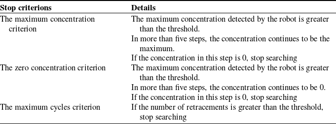
The zigzag–Silkworm algorithm introduces multiple termination criteria as shown in Table VI.
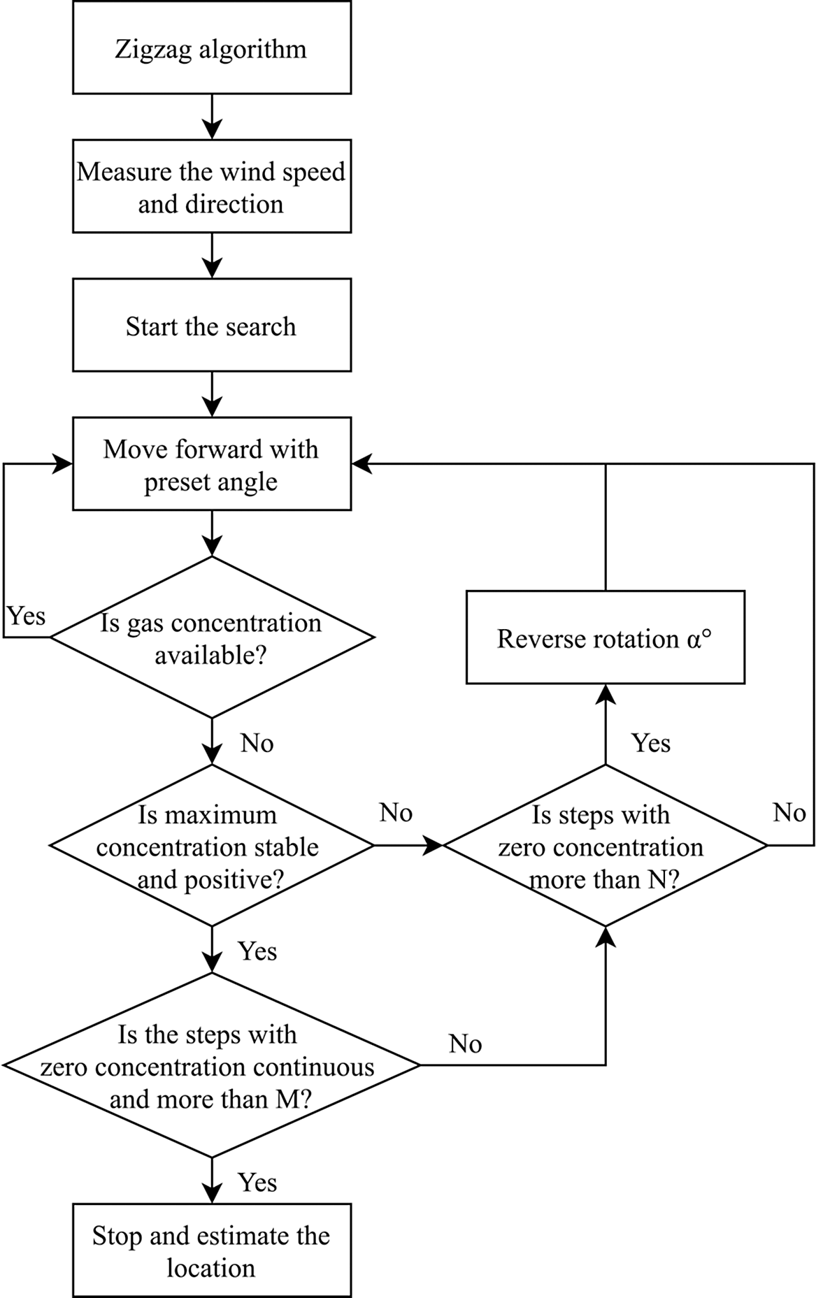
Figure 4. The flow chart of Zigzag algorithm.
Table IV. Pseudocode of Zigzag algorithm.
4. Results
4.1. Results of simulation cases
4.1.1. Results of Silkworm and Zigzag algorithm
Before the outdoor experiments, a series of numerical simulation experiments with Silkworm, Zigzag, and zigzag–Silkworm algorithms was carried out. The concentrations in the simulation scenarios were calculated with a Gaussian dispersion model coupled with some random noises. Figure 5 shows the simulation results of Silkworm (Fig. 5(a) and (b)) and Zigzag (Fig. 5(c) and (d)) with different starting points.
Table V. Pseudocode of zigzag–Silkworm algorithm.

Table VI. The stopping criterions used in the zigzag–Silkworm algorithm.

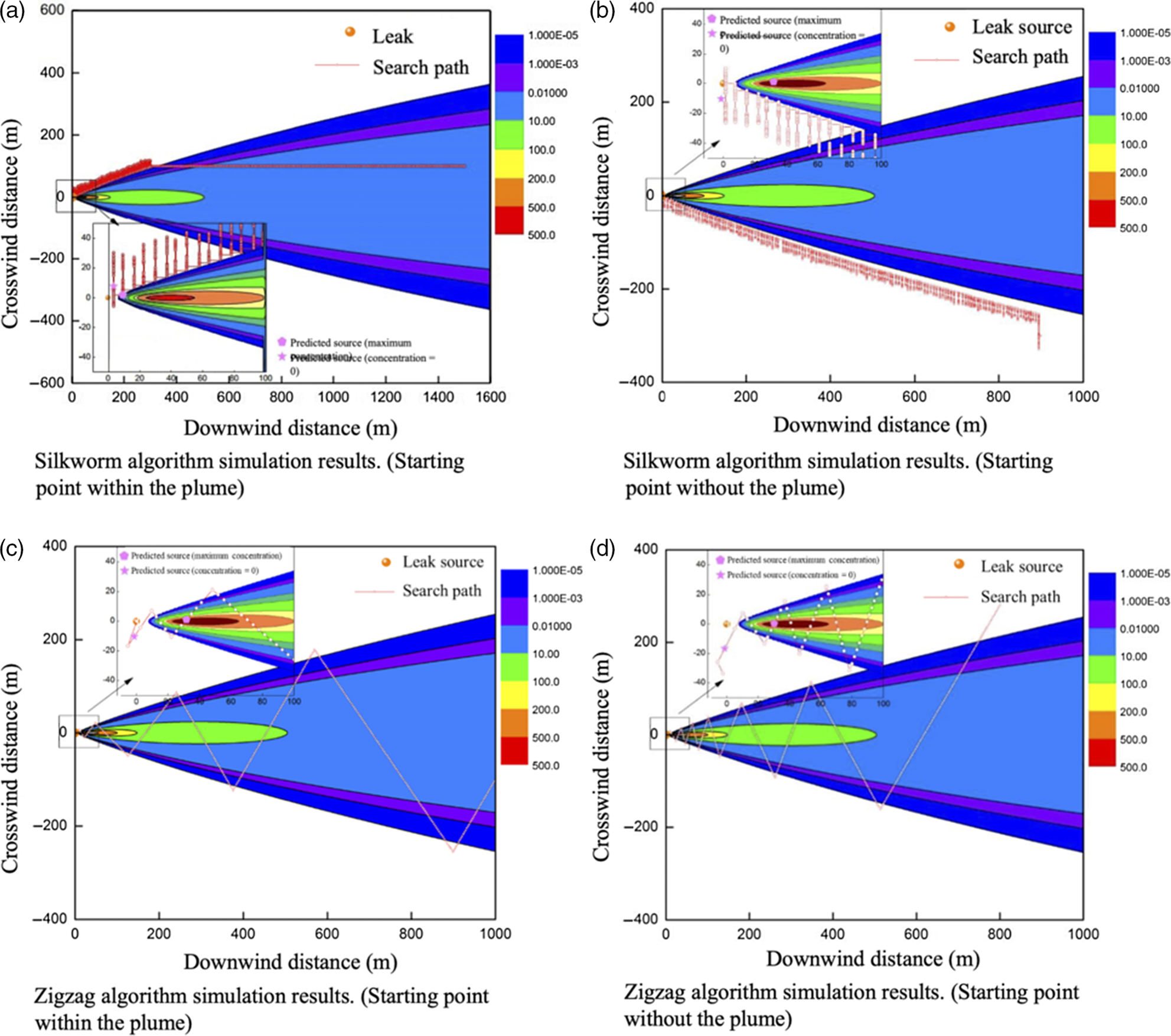
Figure 5. Simulation results of Silkworm and Zigzag algorithms. (a) Result of Silkworm with starting point in the plume. (b) Result of Silkworm with starting point out the plume. (c) Result of Zigzag with starting point in the plume. (d) Result of Zigzag with starting point out the plume.
4.1.2. Results of zigzag–Silkworm algorithm
Figures 6 and 7 show the whole process of source tracing simulations with zigzag–Silkworm algorithm. In Fig. 6(a), the starting point, (900, 50), is inside the plume. Figure. 6(b) and (c) indicate the variation of concentration and concentration gradient during the process. Figure 7(a) demonstrates the results of the case with the starting point out of the plume (900, −300).The results of Fig. 7(b) and (c) indicate that the maximum concentration and concentration gradient are located near the leak source. Hence, the maximum concentration and the maximum concentration gradient can be used as termination criteria in this case.
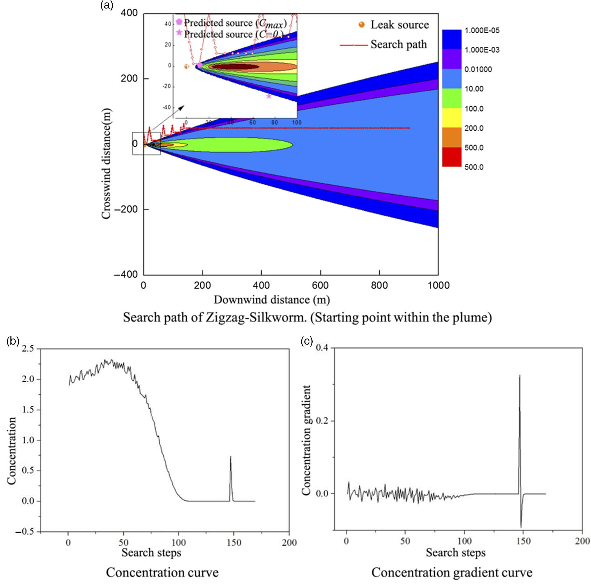
Figure 6. The process of simulatedtracing process with zigzag–Silkworm algorithm with the starting point in the plume. (a) search path with zigzag–Silkworm algorithm. (b) Concentration during the search process, and (c) Concentration gradient during the search process.
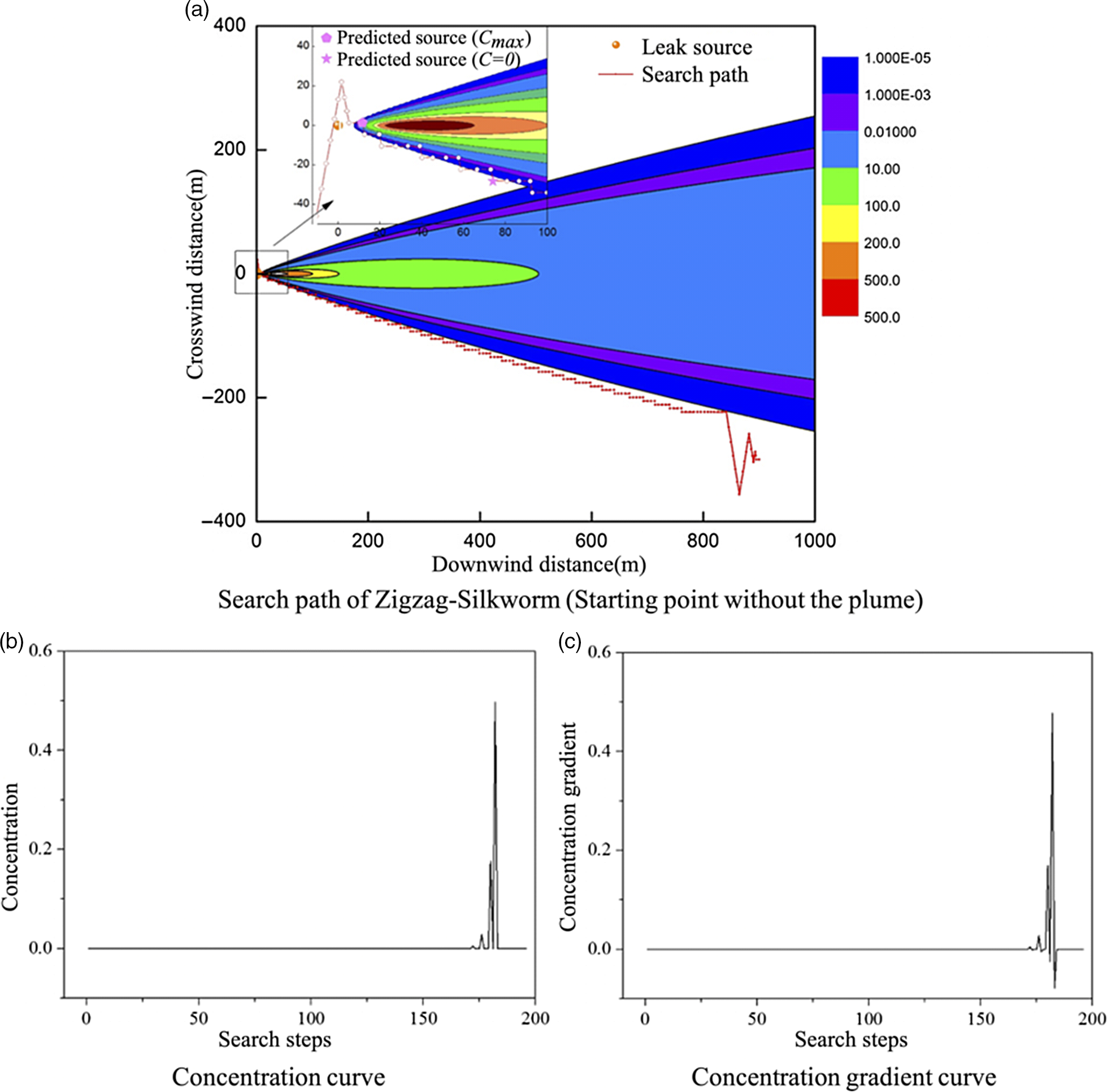
Figure 7. The process of simulatedtracing process with zigzag–Silkworm algorithm with the starting point out of the plume. (a) Searching path with zigzag–Silkworm algorithm w. (b) Concentration during the search process, and (c) Concentration gradient during the search process.
4.2. Experimental cases
4.2.1. The experiments with Silkworm algorithm
The outdoor experiments of emission source tracing with Silkworm algorithm were carried out in this research. Figure 8 shows the path of the robot in one experiment. The plume in the figure is used to symbolically display the concentration distribution, which was obtained during simulation calculation with a Gaussian dispersion model. Thus, it does not represent the actual concentration distribution in the experiments, as the same in the figures of the following sections. The robot’s starting point is at (0,0). Driven by the Silkworm algorithm, the robot moved with swinging perpendicular to the wind direction. When the robot met the plume, it moved forward in an upwind direction. In the experiments, the distribution of the plume was uncertain because of the variations of environmental conditions. At this time, the robot may not be able to detect the gas concentration. Thus, the robot repeated the swinging movement until entering the plume. The robot looped back and forth. Finally, it stopped searching when the stop criterion was reached.
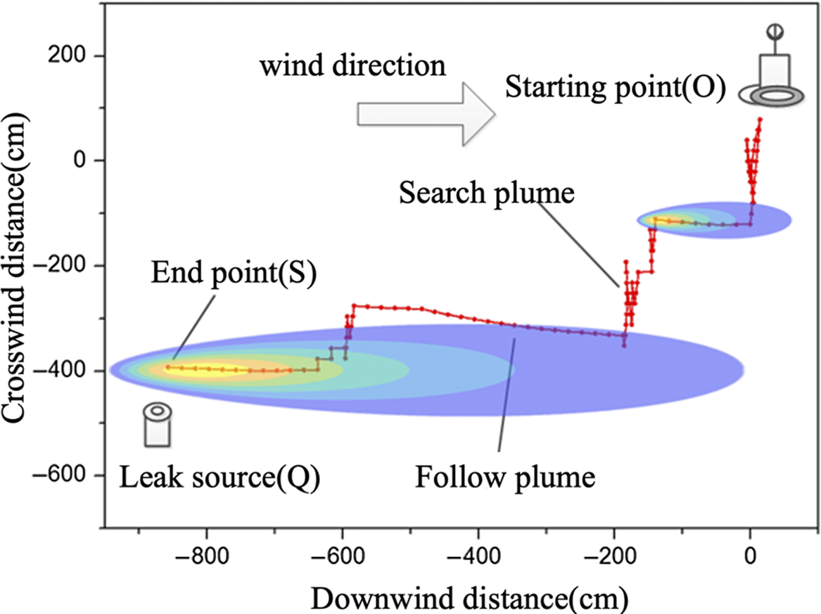
Figure 8. The source tracing process with Silkworm algorithm.
For the experiment with Silkworm algorithm shown in Fig. 8, the leak source was located at (−900, −400). The positioning error Le within the range of 10 ×20 m2 is 24 cm. The total distance of the source tracing process L was 2320 cm, and the ratio L/L 0 is 2.36, where L 0 is the straight distance from the start point to the source. In our research, some tracing experiments with Silkworm algorithm were failed because of too much unstable atmosphere and the inability to find the plume. For failed cases, the area swept by the robot was not enough to touch the plume, therefore, the robot stopped searching after exceeding the maximum time of swing set with default.
4.2.2. The experiments with Zigzag algorithm
Figure 9 shows one experiment with the Zigzag algorithm to trace the source. The robot started to search at the point (0,0). It moved continuously with the preset angle, and then it entered the plume and moved out of the plume. When the robot did not detect the gas concentration, it deflected with a certain angle in the reverse direction, and kept moving. Then it traced the source with the form of zigzag between the boundaries of the plume until approaching near the source.
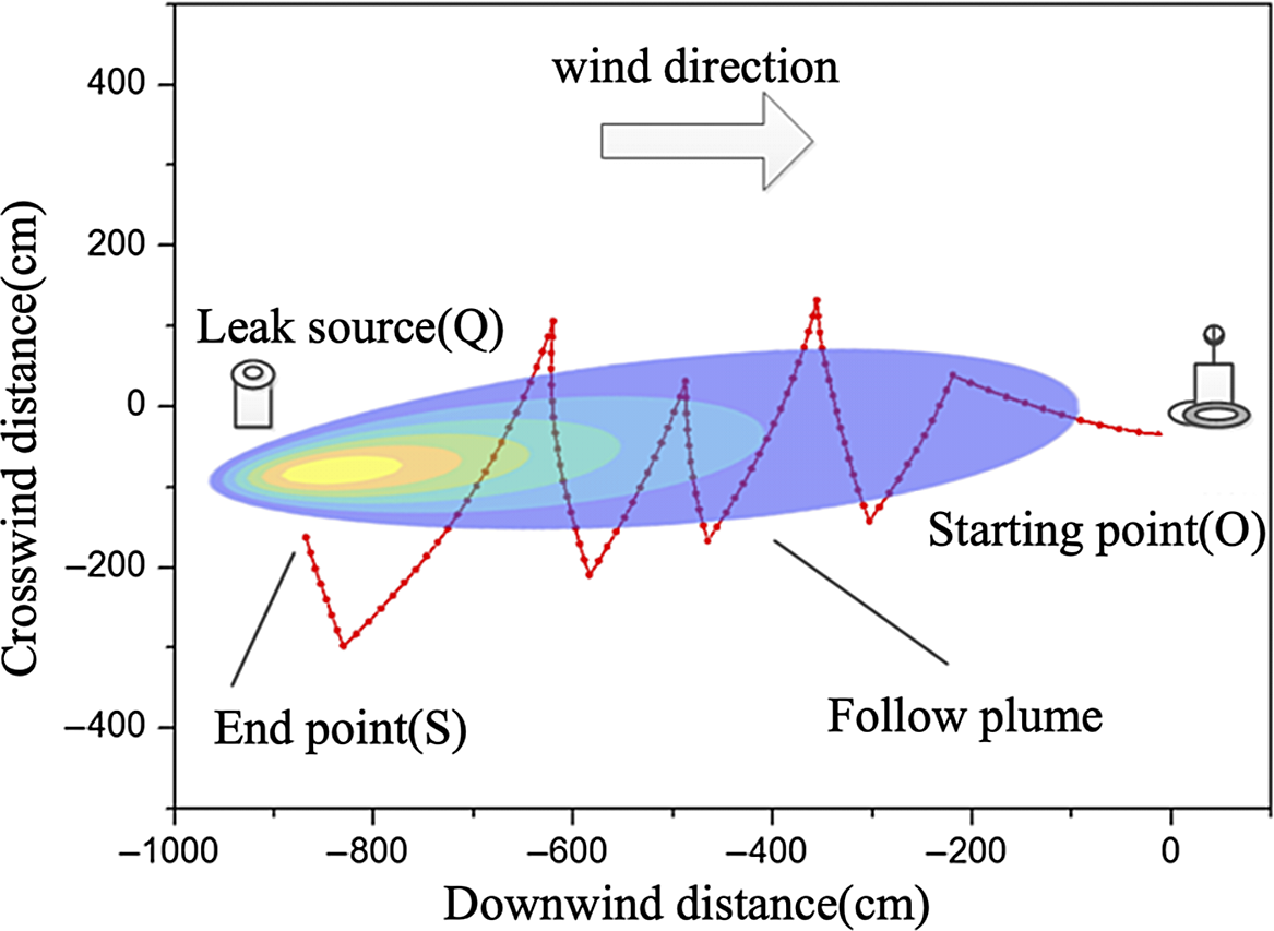
Figure 9. The source tracing process with Zigzag algorithm.
For the experiment with the Zigzag algorithm shown in Fig. 9, the location of the leak source was at (-900,100). The positioning error L e was 49 cm. The total distance of tracing process L is 2400 cm, and the ratio L/L 0 is 2.65. Compared with the results in Figs. 7 and 8, the search efficiency of Zigzag algorithm is higher than that of Silkworm algorithm. However, under certain variable atmospheric conditions, the robot with neither the Zigzag nor the Silkworm algorithm could find the boundary of the gas plume and thus the robot may fail to trace the source. Thus, the source tracing algorithms should be improved.
4.2.3. The experiments with zigzag–Silkworm algorithm
Figure 10 shows the search path of the robot to trace the emission source with zigzag–Silkworm algorithm in a certain outdoor experiment. The starting point was at (0,0). The robot swung in the form of the zigzag with increasing amplitude toward the upwind direction. After entering the plume, it moved along the upwind direction. However, the robot may exceed and move across the plume area. Thus, it did not detect the gas concentration. At this time, the robot swung and searched again. Finally, the tracing process was terminated when the stopping criterions were met. In Fig. 10, the location of the leakage source was at (−800, −200) and the tracing error L e is 44 cm. The total distance of the source tracing process L was 1600 cm, and the L/L 0 was 1.94.
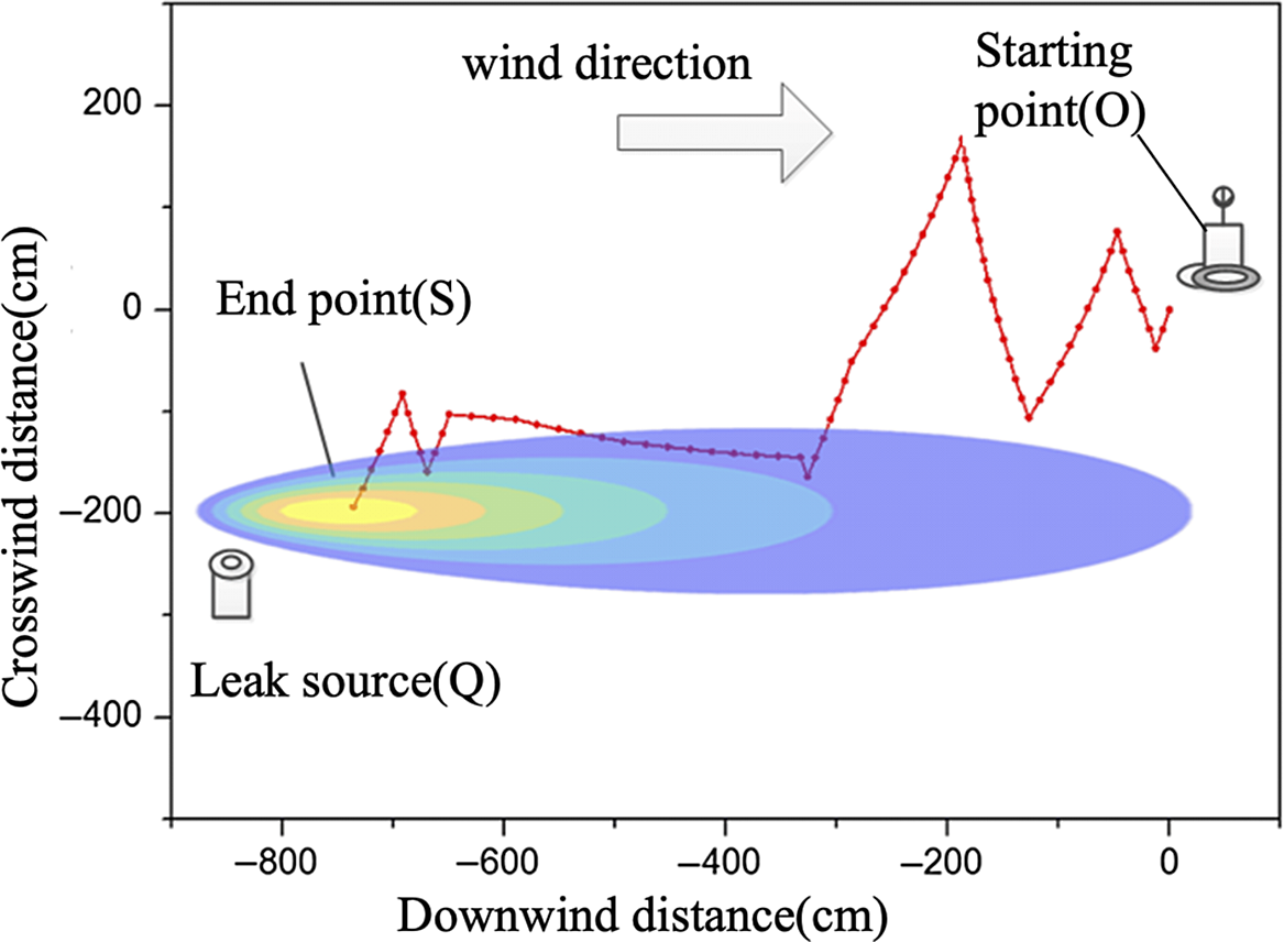
Figure 10. The source tracing process with zigzag–Silkworm algorithm.
4.3. Tracing with Artificial Olfactory System (AOS)
In some cases, the compositions of the leaking gas are unpredictable, for example, sudden gas leakage in chemical industry park, which brings difficulties to tracing the source. The identification of the gas composition in the gas leakage emergencies is important in source tracing and is of great significance for analyzing the leakage risk and handling the accidents in time. Traditional sensors used in gas detection, for example, metal oxide gas sensors, have cross-response for different gases. Thus, they are limited in single detecting object and low gas recognition accuracy. The artificial olfaction system (AOS) imitates the principle of animal’s olfactory ability. It utilizes multidimensional information from sensor array and combines it with pattern recognition algorithms to identify different gases based on the same detection module. In this research, an AOS was designed with sensor array and support vector machine (SVM). The sensor array included three gas sensors with different responses, which were MQ-3 ethanol sensor, MQ-5 combustible gas sensor, and FIGARO_TGS831 alkane gas sensor.
First, a predictive model needs to be established based on experiments in the laboratory. The gas sensor array was placed in a fuming cupboard to detect different gases, including ethanol, ammonia, and n-pentane, released from the nebulizer. In this case, only the gas compositions were required to identify qualitatively, the concentrations were not considered. After noise filtering and normalizing, the collected data were used to train the prediction model with the SVM method. LibSVM developed by Chih-Jen Lin was used in this research [Reference Chang and Lin42,Reference Fan, Chen and Lin43]. The polynomial kernel function was selected as the kernel function of the SVM. The parameter Γ for the kernel function is 0.5. The data set training/test ratio is 5:1 (4500 samples in total). All computation was processed with MATLAB 2019b.
The classification results are demonstrated in Fig. 11. Three kinds of gases can be classified with the SVM model with an accuracy of 100% in the laboratory experiments as shown in Fig. 11(a), (b), (c) and (d). Hence, the AOS designed in this research can be used as a module on the source tracing robot to identify gas components.
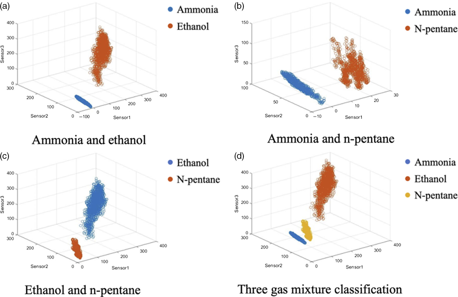
Figure 11. Classification results with pre-trained SVM model for gas samples. (a) Ammonia and ethanol. (b) Ammonia and n-pentane. (c) Ethanol and n-pentane, and (d) All these three gases.
In order to verify the ability of gas recognition during the source tracing in outdoor experiments, the AOS tested in the library was transplanted to the source tracing robot. The liquid of ammonia and ethanol were controlled to release as the leakage sources. The tracing path of the mobile robot equipped with the AOS is shown in Fig. 12(a) and (b).
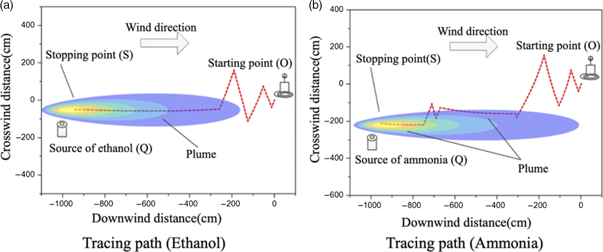
Figure 12. The source tracing paths of mobile robots equipped with AOS in outdoor experiments. (a) Tracing path for ethanol. (b) Tracing path for ammonia.
The positions of nonzero concentration detected in the source tracing process were taken as the samples. There were155 nonzero concentration points extracted from the ammonia experiments and 354 points from the ethanol experiments. Then, the components of the emissions were identified with the pre-trained SVM model. The recognition result shows that the accuracy of the AOS designed in this research to identify ammonia and ethanol in the source tracing experiments is 99.02%, as demonstrated in Fig. 13. Hence, the robot set with both source tracing algorithm and AOS has capability to find the leakage source successfully following with identifying the gas components accurately during the source tracing process.
Additionally, we developed a graphical user interface (GUI) based on MATLAB to demonstrate the information during the source tracing, including the search path, the concentrations, and gas recognition results, as shown in Fig. 14.
Table VII. Statistic results with simulation cases for different algorithms.
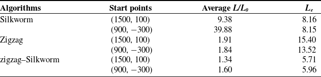
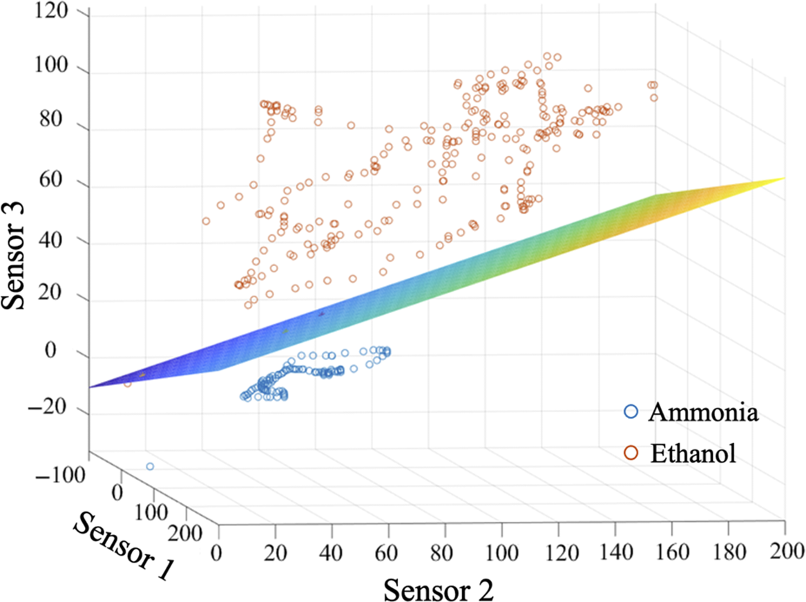
Figure 13. Classification of ammonia and ethanol by AOS in the outdoor experiments.
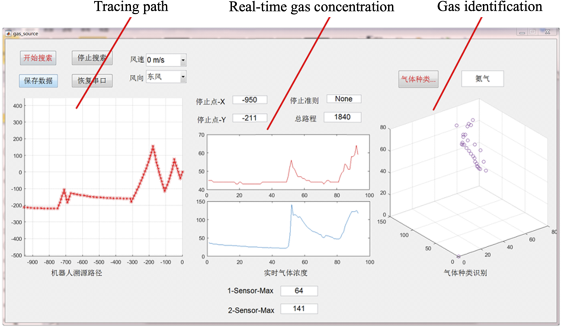
Figure 14. Graphical user interface (GUI) of source tracing.
Table VIII. Statistic results of the outdoor source tracing experiments with three algorithms.
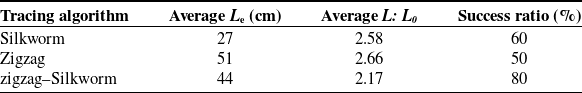
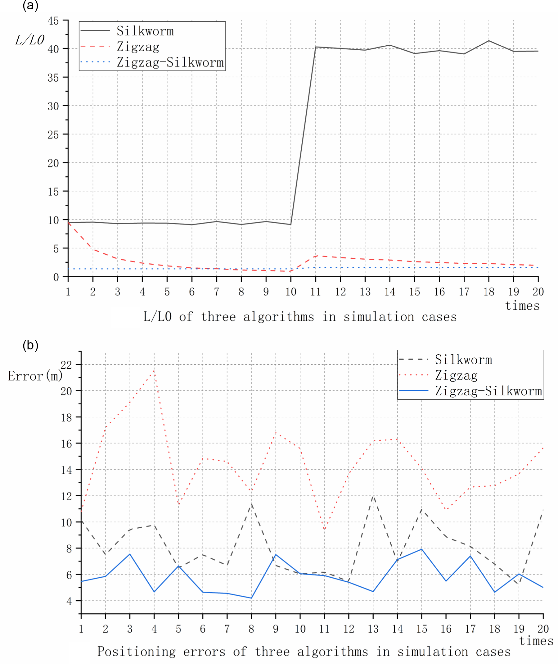
Figure 15. Comparisons of three source tracing algorithms. (a) L/L0 of three algorithms in simulation cases. (b) Positioning errors of three algorithms in simulation cases.
Table IX. Comparison of different gas recognition algorithms.
4.4. Discussion
4.4.1. Comparison of different source tracing algorithms
In order to evaluate the performance of different source tracing algorithms with statistical results, the source tracing with different starting points was simulated many times. All simulation results were summarized in Table VII, where the starting point (1500, 100) is located in the plume and the starting point (900, −300) is located outside the plume. Each source tracing algorithm was calculated 20 times. In this research, the parameter L/L 0 was defined to compare the efficiency of different algorithms. The ratio of the tracing length to the straight-line distance can eliminate the influence of absolute starting point. The less value of L/L 0 , the higher of tracing efficiency is. L e represents the deviation error of the estimation from the actual source. Figure 15 shows that the zigzag–Silkworm performs better than Silkworm and Zigzag in both searching the efficiency (Fig. 15(a)) and positioning accuracy (Fig. 15(b)) in the case of simulation.
On the other hand, the source tracing experiments with Silkworm, Zigzag, and zigzag–Silkworm algorithms were tested 10 times for each. The statistical results of the experiment are shown in Table VIII. The cases where the robot did not find the plume during the whole process were only counted to calculate the success ratio. The comparison results show that the tracing error of Silkworm is the lowest among three algorithms, but the success ratio is only 60% for Silkworm algorithm. Moreover, Zigzag algorithm has the worst performance in both positioning error and search efficiency, and the success ratio is only 50%, even lower than Silkworm in our tests. Although the zigzag–Silkworm algorithm proposed in this research has a slightly higher positioning error than the Silkworm, the search efficiency was greatly improved and the success ratio reached to 80% for zigzag–Silkworm.
According to the results of simulation and experiments, the positioning accuracy and success ratio are not greatly affected by the starting point. The starting point mainly affects the efficiency of the source tracing process, especially the process to find valid plumes. All three algorithms guided the robot to move in an upwind direction and the wind direction varied in different tests. Moreover, the experiments were not completed on the same day. Thus, it was difficult to make sure that the conditions were the same for different experiments. Therefore, the robot started from different positions to make sure the initial positions were in an upwind direction in the experiments. But the evaluation results for location efficiency and error based on the parameters of L/L 0 and L e were not impacted by the initial points greatly. Therefore, the results from different tests in this research were feasible and believable.
Hence, the excellent performances of zigzag–Silkworm in terms of positioning error, search efficiency, and success ratio prove that it has a good application prospect.
4.4.2. Comparison of component identification with different machine leaning models
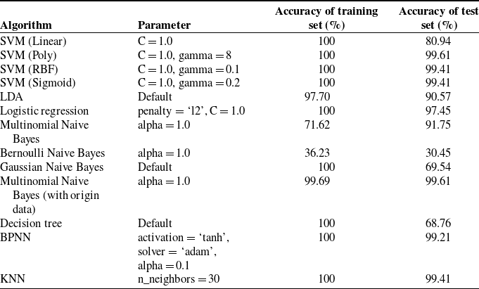
Many machine learning algorithms have been proposed for pattern recognition, such as k-Nearest-Neighbor (KNN), (Support Vector Machine) SVM, Artificial Neural Network (ANN), Linear Discriminant Analysis (LDA). In order to compare the performance of gas identification with AOS, different machine learning models were built to recognize the gases in the source tracing experiments as shown in Table IX. All models listed in Table IX were trained by the data collected in the laboratory, including Ammonia data, ethanol data, and n-pentane data. The ratio of training to test data set is 7:3. The parameters of the models were optimized by ten-fold cross-validation. Finally, the models were tested with the data collected in the outdoor experiments. The comparison results showed that the SVM with poly kernel performed best in gas recognition among different kernel functions. It is also indicated that many machine learning algorithms have excellent performance for gas identification, such as Logistic regression, Multinomial Naive Bayes (with origin data), BPNN, KNN. But the performance of the SVM model with polynomial kernel performed best by considering the prediction accuracy, training speed, and model complexity comprehensively. Hence, it is a potentially good method to identify the gas component with AOS when combined with polynomial kernel SVM model during the source tracing process.
4.4.3. Limitation and application
Although the results of simulation and experiments proved that it is feasible to identify the location and component of the emission event by mobile sensor with bionic algorithm and AOS, there are some limitations for the method proposed in this research. Due to the limitation of the experiment conditions, the searching length of our research was just about 20 m. It will be a challenging issue to trace the emission with too long distance, for example, several miles, because the emission gases may be diluted and the wind direction is varied. Thus, zigzag–Silkworm algorithm is not suitable for tracing the source with too long distance under unstable atmosphere. But the test results showed that it was feasible in short distance tracing. Therefore, it can be used as a patrol inspector in a small area, such as in the gas station or a chemical industry. Moreover, the simulation experiments with the searching distance up to kilometers show that the method discussed in our researches is feasible to locate the source in a long distance if the atmosphere condition is stable.
5. Conclusions
In order to trace the leakage source near the ground, for example, gas leakage near the underground storage site, a mobile source tracing robot was designed. In order to accurately locate the leak source and identify the gas composition during the tracing process, a series of simulation and outdoor experiments with bionic source tracing algorithms were carried out.
The results show that the positioning error of the Silkworm is less than that of Zigzag. Moreover, the tracing efficiency of Silkworm is close to that of Zigzag. However, both Silkworm and Zigzag have some limitations, such as small search areas and high failure ratios. Hence, an improved algorithm was proposed combining the advantages of Silkworm and Zigzag, calling zigzag–Silkworm. The results of simulations and experiments prove that the search efficiency of zigzag–Silkworm has enhanced although its positioning error is slightly higher than Silkworm. Moreover, the success ratio of zigzag–Silkworm was 80% in our experiments.
To identify the components of leakage gas during the source tracing process, an artificial olfactory system (AOS)was designed and equipped on the robot. Then, outdoor experiments were carried out by the source tracing mobile robot based on the AOS and zigzag–Silkworm algorithm. In the outdoor test cases, the accuracy of gas recognition by the robot equipped with AOS was 99%. Therefore, it is feasible to identify gas while tracing the source. Hence, the mobile robot based on AOS and bionic source tracing algorithm is possible to solve the problem of fast recognizing the leakage source in the actual scenarios, for example, oil pipeline leaks, gas storage leaks.
Accordingly, the bionic algorithm can be applied to tracing sources in the open-air atmosphere, although it may fail in a very unstable atmosphere. The AOS provides a possibility for the mobile robot to identify the unknown compositions in accidental leakages. Therefore, the mobile robot based on AOS and bionic source tracing algorithms will be potentially a good tool to trace the source in the fields of hazardous chemical storage, safety inspections, fire rescue, and others like this.
Acknowledgments
Financial support was provided by the National Natural Science Foundation of China (21808181), China Postdoctoral Science Foundation (2019M653651), Shaanxi Provincial Science and Technology Department (2017ZDXM-GY-115), Basic Research Project of Natural Science in Shaanxi province (2020JM-021).