1. Introduction
Visual servos that always help the robots to capture the objects are widely used in industrial automation, spaceflight operation and nuclear reactors. However, the operation accuracy is often impacted by the motion and sensor uncertainties of the manipulator and its visual servo. Traditional methods have been constantly improving the motion accuracy of the actuator and the resolution of the sensors. But errors are widespread and unavoidable. And precision is a relative concept. When the movement error and measurement error of the feedback sensors are smaller than the tolerance, the system could be seen as a deterministic system. But when the tolerance range and the error are on the same order of magnitude, the system can be seen as an uncertain system whose operation has a certain probability of failure. Under special working conditions, such as deep sea, aerospace and nuclear industry, many high-precision industrial sensors cannot be used, and the motion precision and sensing precision cannot fully meet the tolerance requirements.
Many great and classic methods were proposed to solve the capture accuracy problem. There are three kinds of main thinking. The first one is to establish an accurate control system model of the manipulator with right control structure and accurate control parameters. Wang [Reference Wang, Liu, Chen and Mata1] presents an adaptive neural-networks-based scheme for visual servo manipulator system with unmodeled dynamics and external disturbances. Gu [Reference Gu, Wang, Pan and Wu2] approximating the mapping relationship between changes of target image features and robotic joints’ positions with fuzzy-neural networks which instead of Jacobian matrix and weaken the time-delay performance. These two methods all need a process called reinforcement learning to approximate the model with lots of real data and a large amount of calculation time. A database of representative learning samples is employed by Miljkovic´ [Reference Miljkovic, Mitic, Lazarevic and Babic3] so as to speed up the convergence of the neural network and real-time learning of robot behavior. Different from the others, Chang [Reference Chang4] established a two monocular visual servo control model and assembled the phone shells very successfully. To match the kinematics of the robot with the dynamic performance of the vision capture, Khelloufi [Reference Khelloufi, Achour, Passama and Cherubini5] modified the robot driver and modeled and analyzed the designed universal motion structure.
Second, many researches focus on how to reduce the error of visual measurement and movement. Dong [Reference Dong and Zhu6, Reference Dong and Zhu7, Reference Dong and Zhu8] estimates the target’s pose and motion by a vision system using integrated photogrammetry and EKF algorithm. Based on the estimated pose of the target, the desired position of the end-effector is predicted by inverse kinematics and the robotic manipulator is moved incrementally from its current configuration. Phuoc [Reference Dong and Zhu7] propose a method of generating servo motions for a nonholonomic mobile manipulator basing on visual servo, which could not be affected by the excessive platform movement errors at low velocity. Jagersand [Reference Xie, Lynch and Jagersand10] proposed a new IBVS control method with image features from projected lines in a virtual camera image, by which the sensitivity of the capture precision to camera the parameters is reduced. Because the PID parameter of IBVS closed loop control method is difficult to adjust, Kang proposed a novel IBVS method using Extreme Learning Machine (ELM) and Q-learning to solve the problems of complex modeling and selection of the servo gain. Hua [Reference Hua, Liu and Yang11] proposed an immersion and invariance observer to estimate the velocity of the robot. And the stability of the system is proven by using Lyapunov theorem to evaluate the impact of the unknown camera parameters.
Third, accurate calibration methods are often adopted to promote the capture accuracy of the visual servo system including manipulator calibration and visual system calibration. A method of local estimation through training of the feature Jacobian for a manipulator with closed-loop control is presented in Kosmopoulos’ paper [Reference Kosmopoulos12]. The training process is achieved through a non-gaussian robust estimator. Jiang [Reference Jiang and Wang13] calibrate the camera system of space manipulator to improve its locational accuracy. The algorithm fuse the Levenberg–Marqurdt (LM) algorithm and Genetic Algorithm (GA) together dynamically to minimize the error of nonlinear camera model. A novel passivity like error equation [Reference Zhong, Miao and Wang14] of the image features is established by using the spherical camera geometry dynamics with an eye-in-hand configuration to guide the end-effector to the specified position and pose for grabbing.
To sum up, most researches focus on eliminating the system uncertainties with complex nonlinear model, state estimation and accurate calibration. But there is another effective thinking that is not be used in visual servo system. Since error exists everywhere and cannot be avoided absolutely, it is necessary to establish the model of the error in movement decision. Du Toit [Reference Du Toit15, Reference Du Toit and Burdick16] added an error term to the motion model of the mobile robot to obtain an optimized kinematic equation. He creatively proposed the method of nondeterministic modeling and had a profound influence on other scholars. van den Berg [Reference Patil, van den Berg and Alterovitz17, Reference van den Berg, Abbeel and Goldberg18] proposed the method of solving the nondeterministic model based on simultaneous localization and mapping technology. Sun [Reference Sun, Patil and Alterovitz19, Reference Sun, van den Berg and Alterovitz20] further developed the method to optimize the motion of mobile robots and medical probes with known error characteristics in real-time control. For the first time, Qi [Reference Qi, Zhou and Wang21] applied the nondeterministic modeling method to the serial structure robot system. He proposed that when the joint error of the manipulator obeys the Gaussian distribution, the error of the end position also obeys the Gaussian distribution.
Based on the nondeterministic modeling method, this paper studies how to improve the probability of success for a visual capture system with motion and sensor uncertainties. As shown in Fig. 1, the innovation of this paper lies in the motion planning algorithm based on an error nondeterministic model that is added on the basis of the classical PBVS visual servo method [Reference Kang, Chen and Dong22]. By fusing motion error and sensing error, the correlation model between the nondeterministic error distribution at the end of the manipulator in the closed-loop visual servo process and the joint space state of the system is established. Three-dimensional representation of variance matrix in Cartesian space is realized based on probability theory. Based on the error distribution and intelligent optimization strategy, the quantitative measurement for the success probability of the capture motion is obtained, so as to suppress the influence of multi-source errors in the system.
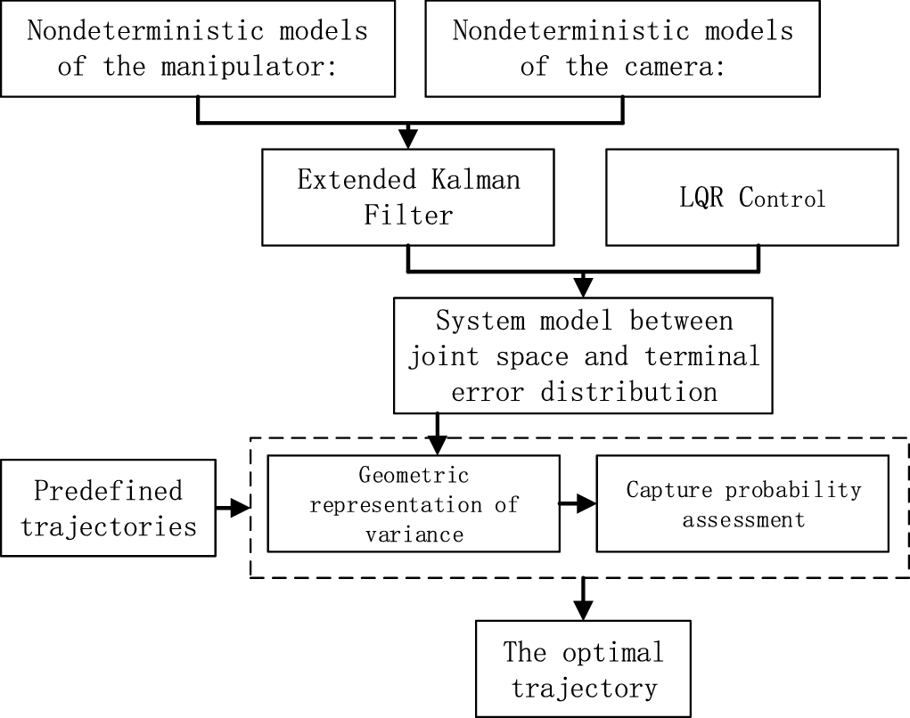
Figure 1. Flow chart of optimal capture trajectory planning method.
The remainder of this paper is organized as follows. We begin by describing system model including motion model and feedback model with uncertainties in Section 2. In Section 3, we present a Bayesian method combing with LQR control to estimate probability of success in manipulator capture. The simulation, experimental results and related discussion are presented in Section 4. Finally, in Section 5, we offer conclusions.
2. Nondeterministic modeling
Usually, when a manipulator is used to capture an object, the position of the end effector can be calculated with forward kinematics. However, since the links are hinged, inevitably, its mechanism has clearance error, deformation error and so on. For the series manipulator, if each joint has errors, the influence of terminal position errors cannot be ignored. In order to improve the capture accuracy, adding external feedback is an effective method. The existence of hand-eye camera in the capture system makes it possible to establish this feedback mechanism. Before capturing, when the camera see the target for the first time, it will plan a trajectory to capture it. However, the manipulator has some error and the capture behavior is not necessarily successful. In the process of capturing, the camera collects the relative pose and posture relation between the target and the end of the manipulator in real time as shown in Fig. 2. Unfortunately, the measured pose and posture of the camera is not very accurate for the measurement system has a range of errors [Reference Pomares, Perea, Jara, García and Torres23].
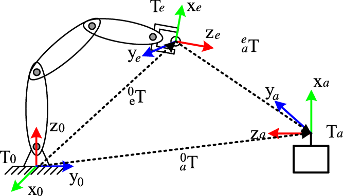
Figure 2. Schematic diagram and coordinates of visual capture.
(a) Nondeterministic system model
When the camera find and prepare to capture a static object, it constructs a closed-loop among the end effector position under the based coordinate of manipulator. It is the closed-loop to construct a feedback and modification process. The motion and sensing errors are too complex to be described by a certain model. Hence, the system model is established with error described by the Gaussian distribution which is most widely used to describe the error distribution in natural chaos.
For the numeral control system such as manipulators and CNC system, the entire control process can be divided into many small control period. In every control period, the control system of the manipulator moves joints from its last state to the objective state which is commanded by the system input. The current system state
 ${\boldsymbol{{x}}_{\boldsymbol{{t}}}}$
is determined by the system state
${\boldsymbol{{x}}_{\boldsymbol{{t}}}}$
is determined by the system state
 ${\boldsymbol{{x}}_{\boldsymbol{{t}} - \textbf{1}}}$
and input
${\boldsymbol{{x}}_{\boldsymbol{{t}} - \textbf{1}}}$
and input
 ${\boldsymbol{{u}}_{\boldsymbol{{t}} - \textbf{1}}}$
in the previous control period. In addition, the motion error
${\boldsymbol{{u}}_{\boldsymbol{{t}} - \textbf{1}}}$
in the previous control period. In addition, the motion error
 ${\boldsymbol{{m}}_{\boldsymbol{{t}}}}$
can also have a significant impact on the state of the system. And then the motion model of the manipulator can be written as
${\boldsymbol{{m}}_{\boldsymbol{{t}}}}$
can also have a significant impact on the state of the system. And then the motion model of the manipulator can be written as
 \begin{align}{\boldsymbol{{x}}_{\boldsymbol{{t}}}} = f\left( {{\boldsymbol{{x}}_{\boldsymbol{{t}} - \textbf{1}}},{\boldsymbol{{u}}_{\boldsymbol{{t}} - \textbf{1}}},\ {\boldsymbol{{m}}_{\boldsymbol{{t}}}}} \right)\,\,{\boldsymbol{{m}}_{\boldsymbol{{t}}}}\sim{\rm{N}}\left( {0,{\boldsymbol{{M}}_{\boldsymbol{{t}}}}} \right) \end{align}
where
 ${\boldsymbol{{m}}_{\boldsymbol{{t}}}}$
is the zero-mean Gaussian motion error of the manipulator at control period
${\boldsymbol{{m}}_{\boldsymbol{{t}}}}$
is the zero-mean Gaussian motion error of the manipulator at control period
 $t$
,
$t$
,
 ${\boldsymbol{{M}}_{\boldsymbol{{t}}}}$
is its variance. Ideally, when the system error is zero.
${\boldsymbol{{M}}_{\boldsymbol{{t}}}}$
is its variance. Ideally, when the system error is zero.
 \begin{align}\boldsymbol{{x}}_t^* = f\left( {\boldsymbol{{x}}_{t - 1}^*,\boldsymbol{{u}}_{t - 1}^*,\textbf{0}} \right)\end{align}
(b) Nondeterministic feedback model
When the external camera is used for sensing, the feedback value
 ${\boldsymbol{{z}}_{\boldsymbol{{t}}}}$
is directly related to the current system state
${\boldsymbol{{z}}_{\boldsymbol{{t}}}}$
is directly related to the current system state
 ${\boldsymbol{{x}}_{\boldsymbol{{t}}}}$
and in the same time affected by the sensing error
${\boldsymbol{{x}}_{\boldsymbol{{t}}}}$
and in the same time affected by the sensing error
 ${\boldsymbol{{n}}_{\boldsymbol{{t}}}}$
. Suppose that the function is
${\boldsymbol{{n}}_{\boldsymbol{{t}}}}$
. Suppose that the function is
 $h$
and the mapping relation can be written as
$h$
and the mapping relation can be written as
 \begin{align}{\boldsymbol{{z}}_{\boldsymbol{{t}}}} = h\left( {{\boldsymbol{{x}}_{\boldsymbol{{t}}}},{\boldsymbol{{n}}_{\boldsymbol{{t}}}}} \right)\qquad {\boldsymbol{{n}}_{\boldsymbol{{t}}}}\sim {\rm{N}}\left( {0,{\boldsymbol{{N}}_{\boldsymbol{{t}}}}} \right) \end{align}
In which,
 $n_t$
is the measurement noise drawn from a zero-mean Gaussian with variance
$n_t$
is the measurement noise drawn from a zero-mean Gaussian with variance
 $N_t$
. In an ideal state,
$N_t$
. In an ideal state,
 ${\boldsymbol{{n}}_{\boldsymbol{{t}}}} = 0$
.
${\boldsymbol{{n}}_{\boldsymbol{{t}}}} = 0$
.
 \begin{align}\boldsymbol{{z}}_t^* = h\left( {\boldsymbol{{x}}_t^*,0} \right)\end{align}
Manipulator is a kind of digital control system which controls its mechanical structure step by step in every control period. In order to simplify the system control process, the nonlinear control model is usually linearized by Taylor expansions in the local space of the system state. Equations (1) and (3) are expended as below.
 \begin{align}{\boldsymbol{{x}}_{\boldsymbol{{t}}}} = f\left( {\boldsymbol{{x}}_{\boldsymbol{{t}} - \textbf{1}}^*,\boldsymbol{{u}}_{\boldsymbol{{t}} - \textbf{1}}^*,0} \right) + {\boldsymbol{{A}}_{\boldsymbol{{t}}}}\left( {{\boldsymbol{{x}}_{\boldsymbol{{t}} - \textbf{1}}} - \boldsymbol{{x}}_{\boldsymbol{{t}} - \textbf{1}}^*} \right) + {\boldsymbol{{B}}_{\boldsymbol{{t}}}}\left( {{\boldsymbol{{u}}_{\boldsymbol{{t}} - \textbf{1}}} - \boldsymbol{{u}}_{\boldsymbol{{\textbf{t}}} - \textbf{1}}^*} \right) + {\boldsymbol{{V}}_{\boldsymbol{{t}}}}{\boldsymbol{{m}}_{\boldsymbol{{t}}}}\end{align}
 \begin{align}{\boldsymbol{{z}}_{\boldsymbol{{t}}}} = h\left( {\boldsymbol{{x}}_{\boldsymbol{{t}}}^*,0} \right) + {H_t}\left( {{\boldsymbol{{x}}_{\boldsymbol{{t}}}} - \boldsymbol{{x}}_{\boldsymbol{{t}}}^*} \right) + {\boldsymbol{{W}}_{\boldsymbol{{t}}}}{\boldsymbol{{n}}_{\boldsymbol{{t}}}}\qquad\qquad\qquad\qquad\quad\qquad\end{align}
where
 \begin{align*}{\boldsymbol{{A}}_{\boldsymbol{{t}}}} & = \frac{{\partial f}}{{\partial x}}\left( {\boldsymbol{{x}}_{\boldsymbol{{t}} - \textbf{1}}^*,\boldsymbol{{u}}_{\boldsymbol{{t}} - \textbf{1}}^*,0} \right) \,\,{\boldsymbol{{B}}_{\boldsymbol{{t}}}} = \frac{{\partial f}}{{\partial u}}\left( {\boldsymbol{{x}}_{\boldsymbol{{t}} - \textbf{1}}^*,\boldsymbol{{u}}_{\boldsymbol{{t}} - \textbf{1}}^*,0} \right)\,\,{\boldsymbol{{V}}_{\boldsymbol{{t}}}} = \frac{{\partial f}}{{\partial m}}\left( {\boldsymbol{{x}}_{\boldsymbol{{t}} - \textbf{1}}^*,\boldsymbol{{u}}_{\boldsymbol{{t}} - \textbf{1}}^*,0} \right)\\[5pt]{\boldsymbol{{H}}_{\boldsymbol{{t}}}} & = \frac{{\partial h}}{{\partial x}}\left( {\boldsymbol{{x}}_{\boldsymbol{{t}}}^*,0} \right)\,\,{\boldsymbol{{W}}_{\boldsymbol{{t}}}} = \frac{{\partial h}}{{\partial n}}\left( {\boldsymbol{{x}}_{\boldsymbol{{t}}}^*,0} \right)\end{align*}
Substitution of Eqs. (2) and (4) into Eqs. (5) and (6) gives
 \begin{align}{\bar{\boldsymbol{{x}}}_{\boldsymbol{{t}}}} = {\boldsymbol{{A}}_{\boldsymbol{{t}}}}{\bar{\boldsymbol{{x}}}_{\boldsymbol{{t}} - \textbf{1}}} + {\boldsymbol{{B}}_{\boldsymbol{{t}}}}{\bar{\boldsymbol{{u}}}_{\boldsymbol{{t}} - \textbf{1}}} + {\boldsymbol{{V}}_{\boldsymbol{{t}}}}{\boldsymbol{{m}}_{\boldsymbol{{t}}}}\qquad\qquad{\boldsymbol{{m}}_{\boldsymbol{{t}}}}\sim {\rm{N}}(0,{\boldsymbol{{M}}_{\boldsymbol{{t}}}})\end{align}
 \begin{align}\!\!{\bar{\boldsymbol{{Z}}}_{\boldsymbol{{t}}}} = {\boldsymbol{{H}}_{\boldsymbol{{t}}}}{\bar{\boldsymbol{{x}}}_{\boldsymbol{{t}}}} + {{\boldsymbol{{W}}}_{\boldsymbol{{t}}}}{\boldsymbol{{n}}_{\boldsymbol{{t}}}}\qquad\qquad\qquad\qquad{\boldsymbol{{n}}_{\boldsymbol{{t}}}}\sim {\rm{N}}(0,{\boldsymbol{{N}}_{\boldsymbol{{t}}}})\ \end{align}
 \begin{align}{\bar{\boldsymbol{{x}}}_{\boldsymbol{{t}}}} = {\boldsymbol{{x}}_{\boldsymbol{{t}}}} - \boldsymbol{{x}}_{\boldsymbol{{t}}}^*\quad {\bar{\boldsymbol{{u}}}_{\boldsymbol{{t}}}} = {\boldsymbol{{u}}_{\boldsymbol{{t}}}} - \boldsymbol{{u}}_{\boldsymbol{{t}}}^*\quad {\bar{\boldsymbol{{z}}}_{\boldsymbol{{t}}}} = {\boldsymbol{{z}}_{\boldsymbol{{t}}}} - h(\boldsymbol{{x}}_{\boldsymbol{{t}}}^*,0)\!\!\quad\qquad\end{align}
where
 ${\bar{\boldsymbol{{x}}}_{\boldsymbol{{t}}}}$
and
${\bar{\boldsymbol{{x}}}_{\boldsymbol{{t}}}}$
and
 ${\bar{\boldsymbol{{u}}}_{\boldsymbol{{t}}}}$
are the deviation of the real system state and input from the predefined values in the trajectory, and
${\bar{\boldsymbol{{u}}}_{\boldsymbol{{t}}}}$
are the deviation of the real system state and input from the predefined values in the trajectory, and
 $\overline{\boldsymbol{{z}}}_{\boldsymbol{{t}}}$
is the deviation of the real measurement value from the ideal value.
$\overline{\boldsymbol{{z}}}_{\boldsymbol{{t}}}$
is the deviation of the real measurement value from the ideal value.
3. Probability prediction
The planned trajectory manipulator can be defined by
 \begin{align}{\rm{\Pi }} = \left( {x_0^{\rm{*}},u_0^{\rm{*}}, \ldots ,x_t^{\rm{*}},u_t^{\rm{*}}, \ldots ,x_{\ell - 1}^{\rm{*}},u_{\ell - 1}^{\rm{*}},x_\ell ^{\rm{*}},u_\ell ^{\rm{*}}} \right)\end{align}
In which,
 ${\rm{\Pi }}$
is a serious of instruction combed by system states
${\rm{\Pi }}$
is a serious of instruction combed by system states
 $x_t^{\rm{*}}$
and input
$x_t^{\rm{*}}$
and input
 $u_t^{\rm{*}}$
, from initial state (
$u_t^{\rm{*}}$
, from initial state (
 $x_0^{\rm{*}},u_0^{\rm{*}}$
) to the end state (
$x_0^{\rm{*}},u_0^{\rm{*}}$
) to the end state (
 $x_\ell ^{\rm{*}},u_\ell ^{\rm{*}}$
).
$x_\ell ^{\rm{*}},u_\ell ^{\rm{*}}$
).
3.1. Trajectory evaluation
In Section 2, the motion model, feedback model and the trajectory with initial and end states are derived. Different trajectories, different motions and feedback errors will affect the accuracy of the manipulator reaching the target position. How to estimate the dynamic error based on the known information is a problem to be solved. As the system is discrete, an Extended Kalman filter (EKF) is selected for system state estimation.
The estimation process of EKF can be written as
 \begin{align}{\tilde{\boldsymbol{{x}}}_{\bar{\boldsymbol{{t}}}}} = {\boldsymbol{{A}}_{\boldsymbol{{t}}}}{\tilde{\boldsymbol{{x}}}_{{\boldsymbol{{t}}} - \textbf{1}}} + {\boldsymbol{{B}}_{\boldsymbol{{t}}}}{\bar{\boldsymbol{{u}}}_{\boldsymbol{{t}} - \textbf{1}}}\qquad\end{align}
 \begin{align}\boldsymbol{{P}}_{\boldsymbol{{t}}}^ - = {\boldsymbol{{A}}_{\boldsymbol{{t}}}}{\boldsymbol{{P}}_{\boldsymbol{{t}} - \textbf{1}}}\boldsymbol{{A}}_{\boldsymbol{{t}}}^{\boldsymbol{{T}}} + {\boldsymbol{{V}}_{\boldsymbol{{t}}}}{\boldsymbol{{M}}_{\boldsymbol{{t}}}}\boldsymbol{{V}}_{\boldsymbol{{t}}}^{\boldsymbol{{T}}}\end{align}
It means that the priori estimate of system state
 $\tilde{\boldsymbol{{x}}}^{\textbf{--}}_{\boldsymbol{{t}}}$
is decided by the optimal estimate in the previous state
$\tilde{\boldsymbol{{x}}}^{\textbf{--}}_{\boldsymbol{{t}}}$
is decided by the optimal estimate in the previous state
 $\tilde{\boldsymbol{{x}}}_{\boldsymbol{{t}}-\textbf{1}}$
and the optimal input
$\tilde{\boldsymbol{{x}}}_{\boldsymbol{{t}}-\textbf{1}}$
and the optimal input
 ${\bar{\boldsymbol{{u}}}_{\boldsymbol{{t}} - \textbf{1}}}$
.
${\bar{\boldsymbol{{u}}}_{\boldsymbol{{t}} - \textbf{1}}}$
.
 $\boldsymbol{{P}}_{\boldsymbol{{t}}}^ - $
is the variance of the priori estimation at stage
$\boldsymbol{{P}}_{\boldsymbol{{t}}}^ - $
is the variance of the priori estimation at stage
 $t$
. And then the correction process is
$t$
. And then the correction process is
 \begin{align}{\boldsymbol{{K}}_{\boldsymbol{{t}}}} = \boldsymbol{{P}}_{\boldsymbol{{t}}}^ - \boldsymbol{{H}}_{\boldsymbol{{t}}}^{\boldsymbol{{T}}}{\left( {{\boldsymbol{{H}}_{\boldsymbol{{t}}}}\boldsymbol{{P}}_{\boldsymbol{{t}}}^- \boldsymbol{{H}}_{\boldsymbol{{t}}}^{\boldsymbol{{T}}} + {\boldsymbol{{W}}_{\boldsymbol{{t}}}}\boldsymbol{{N}}_{\boldsymbol{{t}}}^- \boldsymbol{{W}}_{\boldsymbol{{t}}}^{\boldsymbol{{T}}}} \right)^{ - 1}}\end{align}
 \begin{align}{\tilde{\boldsymbol{{x}}}_{\boldsymbol{{t}}}} = {\tilde{\boldsymbol{{x}}}_{\bar{\boldsymbol{{t}}}}^{-}} + {\boldsymbol{{K}}_{\boldsymbol{{t}}}}\left( {{{\bar{\boldsymbol{{z}}}}_{\boldsymbol{{t}}}} - {\boldsymbol{{H}}_{\boldsymbol{{t}}}}{{\tilde{\boldsymbol{{x}}}}_{\bar{\boldsymbol{{t}}}}}} \right)\qquad\qquad\quad\end{align}
 \begin{align}{\boldsymbol{{P}}}_{\boldsymbol{{t}}} = \left( {\boldsymbol{{I}} - {\boldsymbol{{K}}_{\boldsymbol{{t}}}}{\boldsymbol{{H}}_{\boldsymbol{{t}}}}} \right)\boldsymbol{{P}}_{\boldsymbol{{t}}}^ - \qquad\qquad\qquad\ \ \ \end{align}
where
 ${\boldsymbol{{P}}_{\boldsymbol{{t}}}}$
is the variance of the optimal estimate after the correction process at stage
${\boldsymbol{{P}}_{\boldsymbol{{t}}}}$
is the variance of the optimal estimate after the correction process at stage
 $\boldsymbol{{t}}$
.
$\boldsymbol{{t}}$
.
 ${\boldsymbol{{K}}_{\boldsymbol{{t}}}}$
is the Kalman gain matrix.
${\boldsymbol{{K}}_{\boldsymbol{{t}}}}$
is the Kalman gain matrix.
Since the predefined trajectories are states and inputs, when the closed-loop system performs state estimation, the state feedback of the current cycle adjusts the system input through closed loop control. The purpose of the closed loop is to minimize the cumulative error between the actual value and predefined value of the system states and the inputs, as shown in Eq. (16).
 \begin{align}{\rm{min}}\left( {\mathop \sum \limits_{t = 0}^\ell \left({\bar{\boldsymbol{{x}}}_{\boldsymbol{{t}}}^{\boldsymbol{{T}}}\boldsymbol{{C}}{{\bar{\boldsymbol{{x}}} }_{\boldsymbol{{t}}}} + \bar{\boldsymbol{{x}}} _{\boldsymbol{{t}}}^\boldsymbol{{T}}\boldsymbol{{D}}{{\bar{\boldsymbol{{u}}} }_{\boldsymbol{{t}}}}} \right)} \right)\end{align}
 \begin{align}\boldsymbol{{C}} = \alpha \cdot \boldsymbol{{I}}\end{align}
 \begin{align}\boldsymbol{{D}} = \beta \cdot \boldsymbol{{I}}\end{align}
In which
 $\boldsymbol{{I}}$
is a unit matrix.
$\boldsymbol{{I}}$
is a unit matrix.
 $\alpha $
and
$\alpha $
and
 $\beta $
are two positive represent weights of the system state item and input item. The greater the weight, the stronger the constraint on the error of the corresponding term. The solution of Eq. (16) is the corrected value of the closed-loop control. Its solution process is a typical LQR control problem. The correction of the input
$\beta $
are two positive represent weights of the system state item and input item. The greater the weight, the stronger the constraint on the error of the corresponding term. The solution of Eq. (16) is the corrected value of the closed-loop control. Its solution process is a typical LQR control problem. The correction of the input
 ${\bar{\boldsymbol{{u}}}_{\boldsymbol{{t}}}}$
can be calculated by the optimal estimate
${\bar{\boldsymbol{{u}}}_{\boldsymbol{{t}}}}$
can be calculated by the optimal estimate
 $\tilde{\boldsymbol{{x}}}_{\boldsymbol{{t}}}$
 \begin{align}{\bar{\boldsymbol{{u}}}_{\boldsymbol{{t}}}} = {\boldsymbol{{L}}_{\boldsymbol{{t}}}}{\tilde{\boldsymbol{{x}}}_{\boldsymbol{{t}}}}\end{align}
where
 ${\boldsymbol{{L}}_{\boldsymbol{{t}}}}$
is a feedback matrix. According to the LQR method,
${\boldsymbol{{L}}_{\boldsymbol{{t}}}}$
is a feedback matrix. According to the LQR method,
 ${\boldsymbol{{L}}_{\boldsymbol{{t}}}}$
can be computed in reverse-chronological order from the last stage
${\boldsymbol{{L}}_{\boldsymbol{{t}}}}$
can be computed in reverse-chronological order from the last stage
 $\ell $
to the first stage 0,
$\ell $
to the first stage 0,
 $t \in \left( {0,\ell } \right)$
.
$t \in \left( {0,\ell } \right)$
.
 \begin{align}{\boldsymbol{{S}}_{\boldsymbol\ell} } = \boldsymbol{{C}}\end{align}
 \begin{align}{\boldsymbol{{L}}_{\boldsymbol{{t}}}} = - {\left( {\boldsymbol{{B}}_{\boldsymbol{{t}} + \textbf{1}}^\boldsymbol{{T}}{\boldsymbol{{S}}_{\boldsymbol{{t}} + \textbf{1}}}{\boldsymbol{{B}}_{\boldsymbol{{t}} + \textbf{1}}} + \boldsymbol{{D}}} \right)^{ - \textbf{1}}}\boldsymbol{{B}}_{\boldsymbol{{t}} + \textbf{1}}^\boldsymbol{{T}}{\boldsymbol{{S}}_{\boldsymbol{{t}} + \textbf{1}}}{\boldsymbol{{A}}_{\boldsymbol{{t}} + \textbf{1}}}\end{align}
 \begin{align}{\boldsymbol{{S}}_{\boldsymbol{{t}}}} = \boldsymbol{{A}}_{\boldsymbol{{t}} + \textbf{1}}^\boldsymbol{{T}}{\boldsymbol{{S}}_{\boldsymbol{{t}} + \textbf{1}}}{\boldsymbol{{B}}_{\boldsymbol{{t}} + \textbf{1}}}{\boldsymbol{{L}}_{\boldsymbol{{t}}}} + \boldsymbol{{A}}_{\boldsymbol{{t}} + \textbf{1}}^\boldsymbol{{T}}{\boldsymbol{{S}}_{\boldsymbol{{t}} + \textbf{1}}}{\boldsymbol{{A}}_{\boldsymbol{{t}} + \textbf{1}}} + \boldsymbol{{C}}\end{align}
substituting Eq. (14) into Eq. (19), it can be got that
 \begin{align}\left[\begin{array}{c} {\boldsymbol{{x}}_{\boldsymbol{{t}}}}\\[3pt] {{\boldsymbol{{u}}_{\boldsymbol{{t}}}}} \end{array}\right] = \left[\begin{array}{c@{\quad}c} \boldsymbol{{I}} & 0 \\[3pt] 0 & {{\boldsymbol{{L}}_{\boldsymbol{{t}}}}}\end{array} \right] \left[\begin{array}{c} {{{\bar{\boldsymbol{{x}}}}_{\boldsymbol{{t}}}}} \\[3pt] {{{\tilde{\boldsymbol{{x}}}}_{\boldsymbol{{t}}}}} \end{array} \right] + \left[ \begin{array}{c} {\boldsymbol{{x}}_{\boldsymbol{{t}}}^{\boldsymbol\ast}} \\[3pt] {\boldsymbol{{u}}_{\boldsymbol{{t}}}^{\boldsymbol\ast}} \end{array}\right]\end{align}
 \begin{align}\left[ \begin{array}{c}{{\boldsymbol{{x}}_{\boldsymbol{{t}}}}}\\[3pt]{{\boldsymbol{{u}}_{\boldsymbol{{t}}}}}\end{array} \right] \sim \boldsymbol{{N}}\left(\left[\begin{array}{c}{\boldsymbol{{x}}_{\boldsymbol{{t}}}^{\boldsymbol\ast}}\\[3pt]{\boldsymbol{{u}}_{\boldsymbol{{t}}}^{\boldsymbol\ast}}\end{array} \right], {\boldsymbol\kappa _{\boldsymbol{{t}}}}{\boldsymbol{{R}}_{\boldsymbol{{t}}}}\boldsymbol\kappa _{\boldsymbol{{t}}}^\boldsymbol{{T}}\right), {\boldsymbol\kappa _{\boldsymbol{{t}}}} = \left[ {\begin{array}{c@{\quad}c}\boldsymbol{{I}} & 0\\[3pt]0 & {{\boldsymbol{{L}}_{\boldsymbol{{t}}}}}\end{array}} \right]\end{align}
From Eq. (24), the prior distribution of the movement state
 ${\boldsymbol{{x}}_{\boldsymbol{{t}}}}$
and the system input
${\boldsymbol{{x}}_{\boldsymbol{{t}}}}$
and the system input
 ${{\boldsymbol{{u}}}_{\boldsymbol{{t}}}}$
are specified.
${{\boldsymbol{{u}}}_{\boldsymbol{{t}}}}$
are specified.
 ${\boldsymbol{{R}}_{\boldsymbol{{t}}}}$
is the covariance of
${\boldsymbol{{R}}_{\boldsymbol{{t}}}}$
is the covariance of
 $\left[\overline{\boldsymbol{{x}}}_{\boldsymbol{{t}}}\quad \tilde{\boldsymbol{{x}}}_{\boldsymbol{{t}}}\right]^{\rm T}$
with which the trajectory at every stage can be estimated with Eqs. (23) and (24).
$\left[\overline{\boldsymbol{{x}}}_{\boldsymbol{{t}}}\quad \tilde{\boldsymbol{{x}}}_{\boldsymbol{{t}}}\right]^{\rm T}$
with which the trajectory at every stage can be estimated with Eqs. (23) and (24).
Substitute Eqs. (19)–(22) into Eq. (24):
 \begin{align}& \left[ \begin{array}{c}\overline{\boldsymbol{{x}}}_{\boldsymbol{{t}}}\\[3pt]\tilde{\boldsymbol{{x}}}_{\boldsymbol{{t}}}\end{array} \right] = \left[\begin{array}{c@{\quad}c}{\boldsymbol{{A}}}_{{\boldsymbol{{t}}}} & {\boldsymbol{{B}}}_{{\boldsymbol{{t}}}}{\boldsymbol{{L}}}_{{\boldsymbol{{t}}}-\textbf{1}}\\[3pt]{\boldsymbol{{K}}}_{{\boldsymbol{{t}}}}{\boldsymbol{{H}}}_{\boldsymbol{{t}}}{\boldsymbol{{A}}}_{\boldsymbol{{t}}} & {\boldsymbol{{A}}}_{\boldsymbol{{t}}} + {\boldsymbol{{B}}}_{\boldsymbol{{t}}}{\boldsymbol{{L}}}_{{\boldsymbol{{t}}}-\textbf{1}} - {\boldsymbol{{K}}}_{\boldsymbol{{t}}}{\boldsymbol{{H}}}_{\boldsymbol{{t}}}{\boldsymbol{{A}}}_{\boldsymbol{{t}}}\end{array}\right]\left[\begin{array}{c}\overline{\boldsymbol{{x}}}_{\boldsymbol{{t}}-\textbf{1}}\\[3pt]\tilde{\boldsymbol{{x}}}_{\boldsymbol{{t}}-\textbf{1}}\end{array}\right] + \left[\begin{array}{c@{\quad}c}{\boldsymbol{{V}}}_{\boldsymbol{{t}}} & 0\\[3pt]{\boldsymbol{{H}}}_{\boldsymbol{{t}}}{\boldsymbol{{H}}}_{\boldsymbol{{t}}}{\boldsymbol{{V}}}_{\boldsymbol{{t}}} & {\boldsymbol{{K}}}_{\boldsymbol{{t}}}{\boldsymbol{{W}}}_{\boldsymbol{{t}}}\end{array}\right]\left[\begin{array}{c}{\boldsymbol{{m}}}_{\boldsymbol{{t}}}\\[3pt]{\boldsymbol{{n}}}_{\boldsymbol{{t}}}\end{array}\right]\nonumber\\[3pt]& \left[ {\begin{array}{c}{{{\boldsymbol{{m}}}_{\boldsymbol{{t}}}}}\\[3pt]{{{\boldsymbol{{n}}}_{\boldsymbol{{t}}}}}\end{array}} \right] \sim {\rm{N}}\left( 0,\left[\begin{array}{c@{\quad}c}{{{\boldsymbol{{M}}}_{\boldsymbol{{t}}}}} {}& 0\\[3pt]0 {}& {\boldsymbol{{N}}}_{\boldsymbol{{t}}}\end{array} \right] \right)\end{align}
 \begin{align}{{\boldsymbol{{R}}}_{\boldsymbol{{t}}}} = {{\boldsymbol{{F}}}_{\boldsymbol{{t}}}}{{\boldsymbol{{R}}}_{{\boldsymbol{{t}}} - \textbf{1}}}{\boldsymbol{{F}}}_{\boldsymbol{{t}}}^{\boldsymbol{{T}}} + {{\boldsymbol{{G}}}_{\boldsymbol{{t}}}}{{\boldsymbol{{Q}}}_{\boldsymbol{{t}}}}{\boldsymbol{{G}}}_{\boldsymbol{{t}}}^{\boldsymbol{{T}}}\qquad\qquad\qquad\qquad\qquad\qquad\qquad\qquad\qquad\qquad\end{align}
where
 $\left[\begin{array}{c}\overline{\boldsymbol{{x}}}_{\boldsymbol{{t}}}\\ \tilde{\boldsymbol{{x}}}_{\boldsymbol{{t}}}\end{array}\right] = \left[\begin{array}{c}\textbf{0}\\ \textbf{0} \end{array}\right]$
and
$\left[\begin{array}{c}\overline{\boldsymbol{{x}}}_{\boldsymbol{{t}}}\\ \tilde{\boldsymbol{{x}}}_{\boldsymbol{{t}}}\end{array}\right] = \left[\begin{array}{c}\textbf{0}\\ \textbf{0} \end{array}\right]$
and
 ${{\boldsymbol{{R}}}_{\boldsymbol{{t}}}} = \left[ {\begin{array}{c@{\quad}c}{{P_0}} {}& 0\\0 & {}0\end{array}} \right]$
.
${{\boldsymbol{{R}}}_{\boldsymbol{{t}}}} = \left[ {\begin{array}{c@{\quad}c}{{P_0}} {}& 0\\0 & {}0\end{array}} \right]$
.
 ${P_0}$
is the initial variance of the system state
${P_0}$
is the initial variance of the system state
 ${P_t}$
which can be set at a relatively large value and would converge to a normal value in the process of estimation.
${P_t}$
which can be set at a relatively large value and would converge to a normal value in the process of estimation.
3.2. Evaluation of uncertainty distribution
The variance matrix is the mathematical expression of the error distribution. It is directly related to the spatial geometric distribution, and the variance also represents the spatial geometric distribution of the error points.
 ${{\boldsymbol{{R}}}_{\boldsymbol{{t}}}}$
is the variance of the system state which is in the joint space of the manipulator. The capture behavior is carried out in Cartesian space, and its success probability also should be evaluated in Cartesian space.
${{\boldsymbol{{R}}}_{\boldsymbol{{t}}}}$
is the variance of the system state which is in the joint space of the manipulator. The capture behavior is carried out in Cartesian space, and its success probability also should be evaluated in Cartesian space.
For stage k of the planned trajectory, the distribution of the end position of the manipulator
 ${\rm{N}}\left( {{{\boldsymbol{{p}}}_{\boldsymbol{{k}}}},{\boldsymbol\Sigma _{\boldsymbol{{k}}}}} \right)$
can be calculated by
${\rm{N}}\left( {{{\boldsymbol{{p}}}_{\boldsymbol{{k}}}},{\boldsymbol\Sigma _{\boldsymbol{{k}}}}} \right)$
can be calculated by
 \begin{align}{{\boldsymbol{{p}}}_{\boldsymbol{{k}}}} = g\!\left( {{{\boldsymbol{{x}}}_{\boldsymbol{{k}}}}} \right)\end{align}
 \begin{align}{\boldsymbol\Sigma _{\boldsymbol{{k}}}} = \;{{\boldsymbol{{J}}}_{\boldsymbol{{k}}}}{\aleph _{\boldsymbol{{k}}}}{{\boldsymbol{{J}}}_{\boldsymbol{{k}}}}\end{align}
 ${{\boldsymbol{{p}}}_{\boldsymbol{{k}}}}$
is the expectation of the end position which can be got by the forward kinematics
${{\boldsymbol{{p}}}_{\boldsymbol{{k}}}}$
is the expectation of the end position which can be got by the forward kinematics
 $g\!\left( \cdot \right)$
,
$g\!\left( \cdot \right)$
,
 ${{\boldsymbol{{J}}}_{\boldsymbol{{k}}}}$
is the Jacobian matrix of
${{\boldsymbol{{J}}}_{\boldsymbol{{k}}}}$
is the Jacobian matrix of
 $g\!\left( \cdot \right){\rm{\;and\;\;}}{\aleph _{\boldsymbol{{k}}}}$
is the variance of
$g\!\left( \cdot \right){\rm{\;and\;\;}}{\aleph _{\boldsymbol{{k}}}}$
is the variance of
 ${{\boldsymbol{{x}}}_{\boldsymbol{{k}}}}$
.
${{\boldsymbol{{x}}}_{\boldsymbol{{k}}}}$
.
The first-three-steps variance matrix
 ${\boldsymbol\Sigma _{\textbf{3,k}}}$
of the
${\boldsymbol\Sigma _{\textbf{3,k}}}$
of the
 ${\boldsymbol\Sigma _{\boldsymbol{{k}}}}$
expresses the distribution of the position coordinates [x, y, z]. The eigenvalue and eigenvector can be obtained by eigen decomposition
${\boldsymbol\Sigma _{\boldsymbol{{k}}}}$
expresses the distribution of the position coordinates [x, y, z]. The eigenvalue and eigenvector can be obtained by eigen decomposition
 ${\rm{Eig}}\left( \cdot \right)$
. Eigenvalue
${\rm{Eig}}\left( \cdot \right)$
. Eigenvalue
 ${{\boldsymbol{{D}}}_{\boldsymbol{{k}}}}$
represents the scaling of the distribution range relative to the standard normal distribution. Eigenvectors
${{\boldsymbol{{D}}}_{\boldsymbol{{k}}}}$
represents the scaling of the distribution range relative to the standard normal distribution. Eigenvectors
 ${{\boldsymbol{{V}}}_{\boldsymbol{{k}}}}$
represents the rotation of the distribution range relative to the standard normal distribution.
${{\boldsymbol{{V}}}_{\boldsymbol{{k}}}}$
represents the rotation of the distribution range relative to the standard normal distribution.
 \begin{align}\left[ {{{\boldsymbol{{V}}}_{\boldsymbol{{k}}}},{{\boldsymbol{{D}}}_{\boldsymbol{{k}}}}} \right] = {\rm{Eig}}\!\left( {{\boldsymbol\Sigma _{\textbf{3,k}}}} \right)\end{align}
The principle and process of the transformation are shown in Fig. 3. The estimation for the end position of the manipulator with an expectation
 ${{\boldsymbol{{p}}}_{\boldsymbol{{k}}}}$
and a variance
${{\boldsymbol{{p}}}_{\boldsymbol{{k}}}}$
and a variance
 ${\boldsymbol{{E}}}{{\boldsymbol{{s}}}_{\boldsymbol{{k}}}}$
can be obtained as follows:
${\boldsymbol{{E}}}{{\boldsymbol{{s}}}_{\boldsymbol{{k}}}}$
can be obtained as follows:
 \begin{align}{\boldsymbol{{E}}}{{\boldsymbol{{s}}}_{\boldsymbol{{k}}}} = {{\boldsymbol{{V}}}_{\boldsymbol{{k}}}} \cdot {\rm{Sqrtm}}\!\left( {{{\boldsymbol{{D}}}_{\boldsymbol{{k}}}}} \right) \cdot {\boldsymbol{{S}}}_{\textbf{0}} + {{\boldsymbol{{p}}}_{\boldsymbol{{k}}}}\end{align}
where
 ${{\boldsymbol{{S}}}_{\textbf{0}}}$
is the standard ball, which is set at the origin point with a three-unit radius.
${{\boldsymbol{{S}}}_{\textbf{0}}}$
is the standard ball, which is set at the origin point with a three-unit radius.
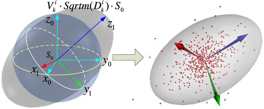
Figure 3. Transformation principle of a variance ellipsoid.
3.3. Capture success probability estimate
The tolerance of the position accuracy is often written in a form of
 ${x_g} \pm h$
, in which
${x_g} \pm h$
, in which
 ${x_g}$
is the aim position and
${x_g}$
is the aim position and
 $h$
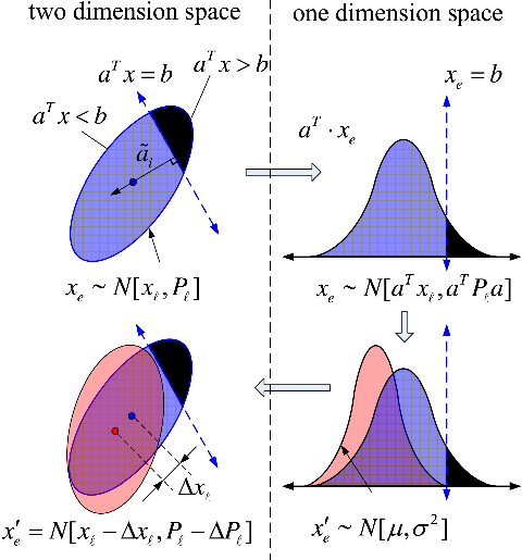
is the allowable error range. For a two dimension aim point, the tolerance range is a rectangle with four lines as shown in Fig. 4. And for a three dimension aim point, the tolerance range is a cube surrounded by six planes. To simplify the narrative, two dimensions distribution and tolerance are taken as an example. The four lines can be seen as four constrains. And then the probability that satisfies the tolerance can be seen as the probability distribution that satisfies the four constraints.
$h$
is the allowable error range. For a two dimension aim point, the tolerance range is a rectangle with four lines as shown in Fig. 4. And for a three dimension aim point, the tolerance range is a cube surrounded by six planes. To simplify the narrative, two dimensions distribution and tolerance are taken as an example. The four lines can be seen as four constrains. And then the probability that satisfies the tolerance can be seen as the probability distribution that satisfies the four constraints.
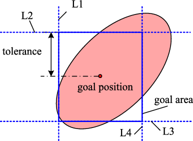
Figure 4. Relationship between tolerance and error distribution.
According to probability theory, the probability value and a new distribution satisfying a certain condition for the current probability distribution can be calculated. The method is shown in Fig. 5.

Figure 5. New distribution satisfying a constraint.
Assuming that the predict distribution is
 ${{\boldsymbol{{x}}}_{\boldsymbol{{e}}}}\sim {\bf{N}}\left[ {{{\boldsymbol{{x}}}_{\boldsymbol{{l}}}},{{\boldsymbol{{P}}}_{\boldsymbol{{l}}}}} \right]$
. A straight line whose equation is
${{\boldsymbol{{x}}}_{\boldsymbol{{e}}}}\sim {\bf{N}}\left[ {{{\boldsymbol{{x}}}_{\boldsymbol{{l}}}},{{\boldsymbol{{P}}}_{\boldsymbol{{l}}}}} \right]$
. A straight line whose equation is
 ${a^T}x = b$
, intersects with the distribution. The part satisfying the constraint can form a new probability distribution, and its expectation
${a^T}x = b$
, intersects with the distribution. The part satisfying the constraint can form a new probability distribution, and its expectation
 $\mu $
and variance
$\mu $
and variance
 ${\sigma ^2}$
in the one-dimensional probability space can be calculated as
${\sigma ^2}$
in the one-dimensional probability space can be calculated as
 \begin{align}{\mu _i} = {{\boldsymbol{{a}}}^{\boldsymbol{{T}}}}{{\boldsymbol{{x}}}_{\boldsymbol\ell} } + \lambda \left( \alpha \right)\sqrt {{{\boldsymbol{{a}}}^{\boldsymbol{{T}}}}{{\boldsymbol{{P}}}_{\boldsymbol\ell}}{\boldsymbol{{a}}}} \end{align}
 \begin{align}{\sigma ^2} = {a^T}Pa(1 - \lambda {\left( \alpha \right)^2} + \alpha \lambda \left( \alpha \right))\end{align}
where
 \begin{align}{\rm{\alpha }} = \frac{{\left( {b - {a^T}{x_\ell }} \right)}}{{\sqrt {{a^T}{P_\ell }a} }}\end{align}
 \begin{align}{\rm{\lambda }}\!\left( {\rm{\alpha }} \right) = \frac{{pdf\left( {\rm{\alpha }} \right)}}{{cdf\left( {\rm{\alpha }} \right)}}\end{align}
 $pdf$
is the standard Gaussian probability distribution function,
$pdf$
is the standard Gaussian probability distribution function,
 $cdf$
is the standard Gaussian cumulative distribution function, and
$cdf$
is the standard Gaussian cumulative distribution function, and
 ${\rm{\lambda }}\!\left( {\rm{\alpha }} \right)$
is their ratio. Then the new distribution
${\rm{\lambda }}\!\left( {\rm{\alpha }} \right)$
is their ratio. Then the new distribution
 ${\boldsymbol{{x}}}^{\prime}_{\boldsymbol{{e}}}\sim {\bf{N}}\left[ {{{\boldsymbol{{x}}}_{\boldsymbol{{l}}}} + \boldsymbol\Delta {\boldsymbol{{x}}},{{\boldsymbol{{P}}}_{\boldsymbol{{l}}}} + \boldsymbol\Delta {{\boldsymbol{{P}}}_{\boldsymbol\ell} }} \right]$
satisfying
${\boldsymbol{{x}}}^{\prime}_{\boldsymbol{{e}}}\sim {\bf{N}}\left[ {{{\boldsymbol{{x}}}_{\boldsymbol{{l}}}} + \boldsymbol\Delta {\boldsymbol{{x}}},{{\boldsymbol{{P}}}_{\boldsymbol{{l}}}} + \boldsymbol\Delta {{\boldsymbol{{P}}}_{\boldsymbol\ell} }} \right]$
satisfying
 ${a^T}x \lt b$
can be transformed from one dimension to two or three dimensions in Cartesian space. Then the probability that satisfy the constrain is
${a^T}x \lt b$
can be transformed from one dimension to two or three dimensions in Cartesian space. Then the probability that satisfy the constrain is
 $cdf\!\left( {\rm{\alpha }} \right)$
.
$cdf\!\left( {\rm{\alpha }} \right)$
.
 \begin{align}\boldsymbol\Delta {\boldsymbol{{x}}} = \frac{{{{\boldsymbol{{P}}}_{\boldsymbol\ell} }{\boldsymbol{{a}}}}}{{{{\boldsymbol{{a}}}^{\boldsymbol{{T}}}}{{\boldsymbol{{P}}}_{\boldsymbol\ell} }{\boldsymbol{{a}}}}}\left( {{{\boldsymbol{{a}}}^{\boldsymbol{{T}}}}{{\boldsymbol{{x}}}_{\boldsymbol\ell} } - \mu } \right)\end{align}
 \begin{align}\boldsymbol\Delta {\boldsymbol{{P}}}_{\boldsymbol{\ell} } = \frac{{{{\boldsymbol{{P}}}_{\boldsymbol\ell} }{\boldsymbol{{a}}}}}{{{{\boldsymbol{{a}}}^{\boldsymbol{{T}}}}{{\boldsymbol{{P}}}_{\boldsymbol\ell} }{\boldsymbol{{a}}}}}\left( {{{\boldsymbol{{a}}}^{\boldsymbol{{T}}}}{{\boldsymbol{{x}}}_{\boldsymbol\ell} }{\boldsymbol{{a}}} - {\sigma ^2}} \right)\frac{{{{\boldsymbol{{a}}}^{\boldsymbol{{T}}}}{{\boldsymbol{{P}}}_{\boldsymbol\ell} }}}{{{{\boldsymbol{{a}}}^{\boldsymbol{{T}}}}{{\boldsymbol{{P}}}_{\boldsymbol\ell} }{\boldsymbol{{a}}}}}\end{align}
The final result is a distribution that satisfies all the constraints. After the final probability that the manipulator arrives at the goal area or captures the aim object is given by
 \begin{align}P{\rm{(}} \cap _0^n{{\boldsymbol{{x}}}_{\boldsymbol{{e}}}} \in \left( {goal\;area} \right)) = \prod\limits_0^n c df\left( {{\alpha _i}} \right)\end{align}
In which,
 ${{\rm{\alpha }}_i}$
is the parameter in Eq. (33), and n is the number of constrains. After calculating a probability contraction according to the constraints, a new probability distribution is obtained. Next time, the obtained probability distribution and the next constraint are calculated together and so on. Finally, the probability distribution satisfying all the constraints is obtained.
${{\rm{\alpha }}_i}$
is the parameter in Eq. (33), and n is the number of constrains. After calculating a probability contraction according to the constraints, a new probability distribution is obtained. Next time, the obtained probability distribution and the next constraint are calculated together and so on. Finally, the probability distribution satisfying all the constraints is obtained.
4. Experiment
A proof manipulator designed for the space station is selected as the experimental platform to verify the effectiveness and correctness of the proposed algorithm.
4.1. Experimental platform and system model
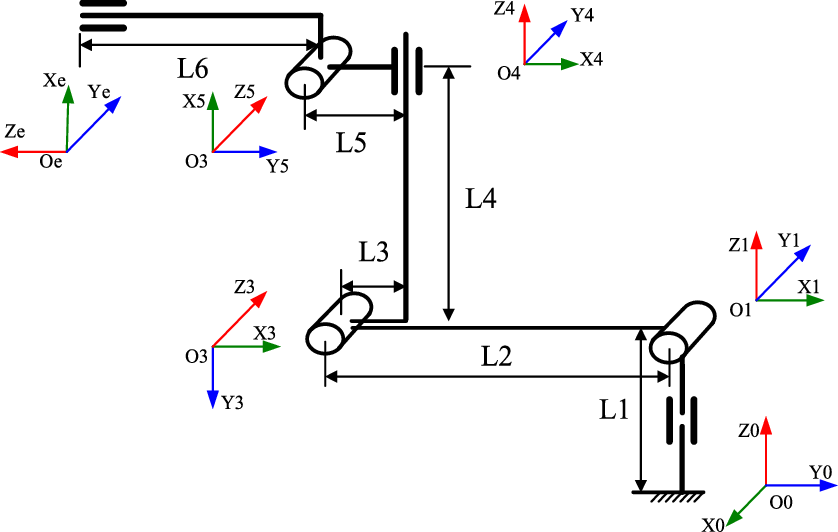
The large 6-dof manipulator designed to works at the space station is shown in Fig. 6(a). Now, the manipulator is just a ground verification system with high precision optical gratings which will be cancelled in the next research stage since the optical gratings are not applicative to the space environment. As we know, the operating accuracy will reduce if the manipulator do not have high precision position sensors. Under that circumstance, the joints have movement error. And in the same time, the visual sensor has sensor error. How to obtain higher operating accuracy for a manipulator under motion and sensor uncertainties with the algorithm proposed in this paper is the objective of our experiment. The manipulator is a 6-dof mechanism with a visual camera at the end effector. The kinematic model is shown in Fig. 7, and the Denavit–Hartenberg (DH) parameters are listed in Table I.
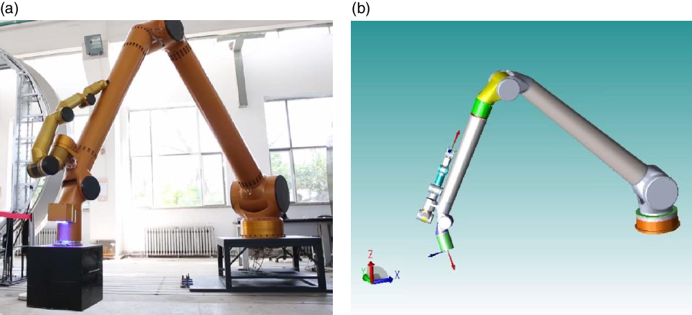
Figure 6. The experimental platform. (a) Actual structure. (b) 3D structural model.
For automatic motion control system such as CNC, manipulators and mobile robots, there are three typical control modes: position control, speed control and torque control. Position control is often used in mobile robots and drilling machine tools. Torque control is often used in textile manufacturing machine and those manipulator controlled by dynamics. Most CNC system and manipulators are controlled by speed control mode.
Table I. DH parameters of the system model.
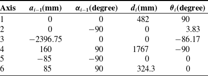

Figure 7. Kinematic model and joint coordinates of the manipulator.
Suppose the trajectory of the manipulator is defined as
 $\chi = \left\{ {x_1^*,x_2^*, \ldots ,x_t^*, \ldots ,x_n^*} \right\}$
. It is the series of instructions for all joints of the manipulator in every control period. Thus, according to the speed control mode, in every control period, the rotation speeds of the joints are determined by
$\chi = \left\{ {x_1^*,x_2^*, \ldots ,x_t^*, \ldots ,x_n^*} \right\}$
. It is the series of instructions for all joints of the manipulator in every control period. Thus, according to the speed control mode, in every control period, the rotation speeds of the joints are determined by
 $\boldsymbol\omega = \left( {{\boldsymbol{{x}}}_{\boldsymbol{{t}}}^* - {\boldsymbol{{x}}}_{{\boldsymbol{{t}}} - \textbf{1}}^*} \right)/\tau $
. So the movement model of the manipulator can be described by a vector mode which means that the current state of the system
$\boldsymbol\omega = \left( {{\boldsymbol{{x}}}_{\boldsymbol{{t}}}^* - {\boldsymbol{{x}}}_{{\boldsymbol{{t}}} - \textbf{1}}^*} \right)/\tau $
. So the movement model of the manipulator can be described by a vector mode which means that the current state of the system
 ${{\boldsymbol{{x}}}_{\boldsymbol{{t}}}}$
is equal to the displacement of a control period with the input velocity
${{\boldsymbol{{x}}}_{\boldsymbol{{t}}}}$
is equal to the displacement of a control period with the input velocity
 $\boldsymbol\tau \cdot \boldsymbol\omega $
added to the previous state of the system
$\boldsymbol\tau \cdot \boldsymbol\omega $
added to the previous state of the system
 ${{\boldsymbol{{x}}}_{{\boldsymbol{{t}}} - \textbf{1}}}$
.
${{\boldsymbol{{x}}}_{{\boldsymbol{{t}}} - \textbf{1}}}$
.
 \begin{align}{{\boldsymbol{{x}}}_{\boldsymbol{{t}}}} = {{\boldsymbol{{x}}}_{{\boldsymbol{{t}}} - \textbf{1}}} + \boldsymbol\tau \cdot \boldsymbol\omega \end{align}
Since the system inevitably has the mechanical error, the trajectory tracking error and the measurement feedback error. Therefore, the control model with system nondeterminacy can bewritten as
 \begin{align}f(x,u,m) = \left[\begin{matrix}{\theta _1} + \tau \left({\omega _1} + {{\tilde \omega }_1}\right)\\[3pt] \vdots \\[5pt] {{\theta _6} + \tau \left({\omega _6} + {{\tilde \omega }_6}\right)} \end{matrix} \right]\end{align}
In which, system state
 $x = \left( {{\theta _1}, \ldots ,{\theta _6}} \right)$
, instruction input
$x = \left( {{\theta _1}, \ldots ,{\theta _6}} \right)$
, instruction input
 $\omega = \left( {{\omega _1}, \ldots ,{\omega _6}} \right)$
and process noise
$\omega = \left( {{\omega _1}, \ldots ,{\omega _6}} \right)$
and process noise
 $m = (\tilde\omega_1, \ldots, \tilde\omega_6) \sim \textbf{N} (0,\sigma_\omega^2 I)$
.
$m = (\tilde\omega_1, \ldots, \tilde\omega_6) \sim \textbf{N} (0,\sigma_\omega^2 I)$
.
As shown in Fig. 1, the transfer matrix between the base coordinate of the manipulator and the visual system coordinate are
 ${}_a^eT$
. The transformation between the end effector matrix
${}_a^eT$
. The transformation between the end effector matrix
 ${}_e^0T$
and the object pose and posture matrix
${}_e^0T$
and the object pose and posture matrix
 ${}_a^0T$
can be written as
${}_a^0T$
can be written as
 \begin{align}{}_a^0T = {}_a^eT \cdot {}_e^0T\end{align}
Thus, the feedback model of the eye-in-hand measurement system is
 \begin{align}h\left( {{x_t},{n_t}} \right) = {}_a^eT \cdot g\left( x \right) + n\end{align}
In which,
 $h\left( {{x_t},{n_t}} \right)$
is the visual measurement value
$h\left( {{x_t},{n_t}} \right)$
is the visual measurement value
 ${}_a^0T$
with error or uncertainties.
${}_a^0T$
with error or uncertainties.
 $g\left( x \right)$
is the end effector matrix calculated by forward kinematics which is the equation expression of
$g\left( x \right)$
is the end effector matrix calculated by forward kinematics which is the equation expression of
 ${}_a^eT$
.
${}_a^eT$
.
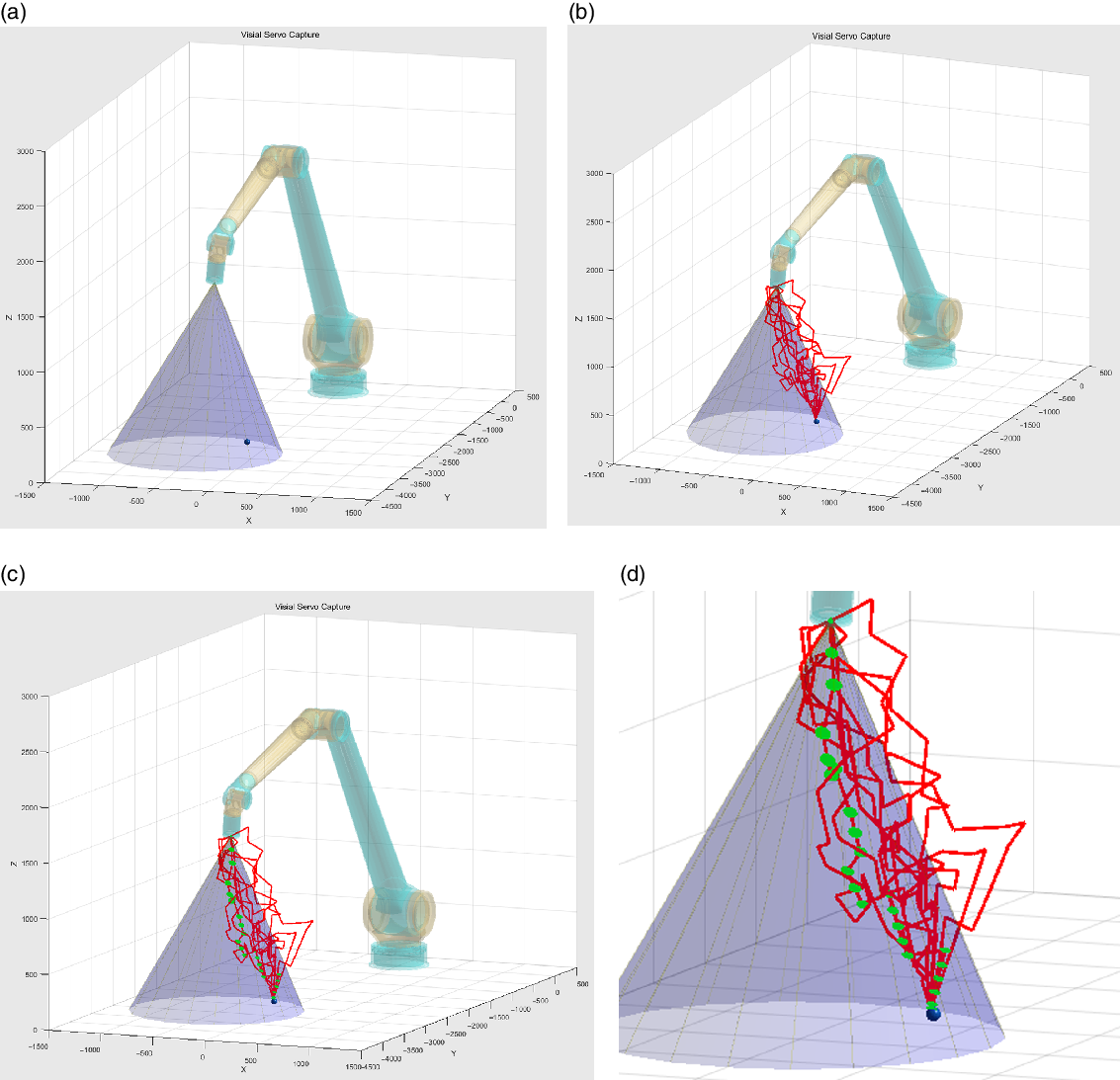
Figure 8. Trajectory generation with non-determinacy (unit:mm).
Corresponding to Eqs. (5) and (6), the derivative parameters of Eqs. (39) and (40) are
 \begin{align}{{\boldsymbol{{A}}}_{\boldsymbol{{t}}}} = diag\left( {1,1,1,1,1,1} \right)\end{align}
 \begin{align}{{\boldsymbol{{B}}}_{\boldsymbol{{t}}}} = {{\boldsymbol{{V}}}_{\boldsymbol{{t}}}} = diag\left( {\tau ,\tau ,\tau ,\tau ,\tau ,\tau } \right)\end{align}
 \begin{align}{{\boldsymbol{{H}}}_{\boldsymbol{{t}}}} = {}_a^eT \cdot {J_t}\left( x \right)\end{align}
 $\tau $
is the control period of the manipulator.
$\tau $
is the control period of the manipulator.
 ${J_t}$
is the Jacobian matrix of the manipulator at stage
${J_t}$
is the Jacobian matrix of the manipulator at stage
 $t $
.
$t $
.
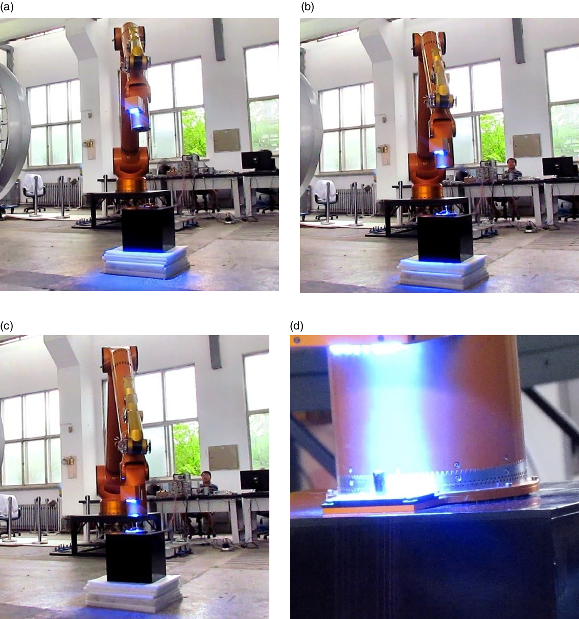
Figure 9. Experimental process. (a) Initial state. (b) Middle state 1. (c) Middle state 2. (d) Final state.
4.2. Probability estimation
According to the design process of the system joint code disc precision and mechanical structure characteristics, the error variance of the six joints is [0.01°; 0.05°; 0.03°; 0.02°; 0.01°; 0.02°] [Reference Jiang and Wang13], and the pose and Euler angle error variance of visual system is [
 ${e_x}$
mm;
${e_x}$
mm;
 ${e_y}$
mm;
${e_y}$
mm;
 ${e_z}$
mm;
${e_z}$
mm;
 ${e_{rx}}$
°;
${e_{rx}}$
°;
 ${e_{ry}}$
°;
${e_{ry}}$
°;
 ${e_{rz}}$
°] [Reference Jiang and Wang13]. According to the research of vision system calibration (Zhang [Reference Zhang, Liu, Tang and Liu24]), the vision errors will change with the relative distance between the visual camera and its object. For our research, the errors can be written as
${e_{rz}}$
°] [Reference Jiang and Wang13]. According to the research of vision system calibration (Zhang [Reference Zhang, Liu, Tang and Liu24]), the vision errors will change with the relative distance between the visual camera and its object. For our research, the errors can be written as
 ${e_x} = {e_y} = 0.005*dis;\;$
 ${e_z} = 0.008*dis;$
 ${e_{rx}} = {e_{rx}} = $
0.035*
${e_{rx}} = {e_{rx}} = $
0.035*
 ${\rm{angl}}{{\rm{e}}^2}$
;
${\rm{angl}}{{\rm{e}}^2}$
;
 ${e_{rz}} = $
0.042*
${e_{rz}} = $
0.042*
 ${\rm{angl}}{{\rm{e}}^2}$
.
${\rm{angl}}{{\rm{e}}^2}$
.
The manipulator starts from the arm joint position [86, 52.17, −158.17, −8, −82, 0] (Unit: degree), which is (−182.443 mm, −2452.23 mm, 33.1061 mm) in Cartesian coordinates. The tolerance of the object capture is assumed to be (−182.443±2.5 mm, −2452.23±2.5 mm, 33.1061±2.5 mm), which is not known and should be measured by the manipulator.
A rapidly explored random trees (RRT) algorithm is adopted to plan trajectories with error ellipsoids at the end position of the manipulator in every control period. The generated trajectories with nondeterminacy described by error distributions are shown in Fig. 8.
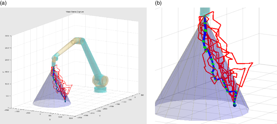
Figure 10. Comparison result of experiment and simulation (unit:mm). (a) Experimental data. (b) Track details.
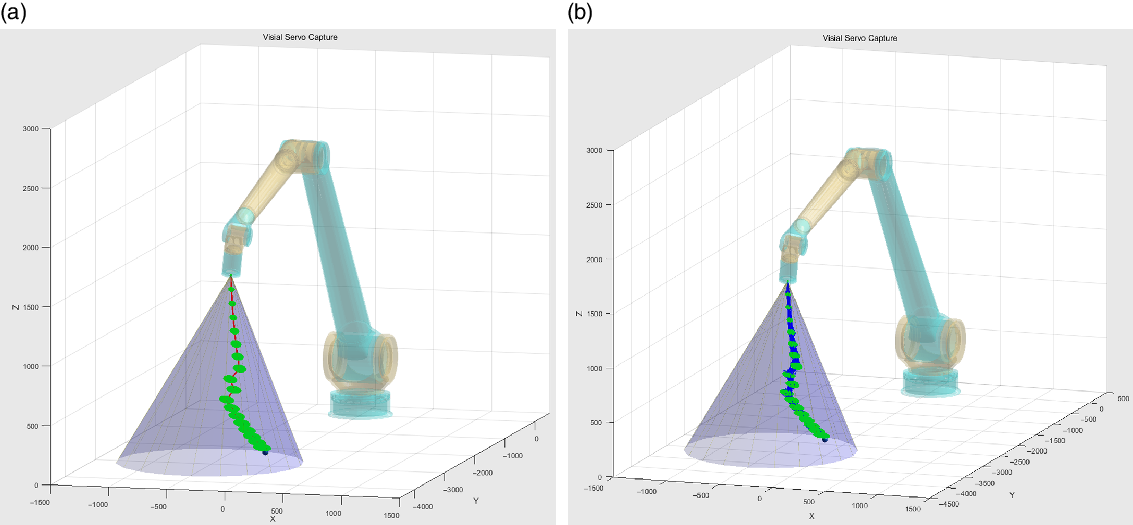
Figure 11. Trajectory generation with an average PBVS visual servo (unit:mm). (a) Distribution prediction of PBVS. (b) Experiment trajectories of PBVS.
4.3. Capture accuracy verification
In order to verify the effectiveness of the algorithm in this paper, an optimal trajectory was selected for repeated execution, so as to compare the fitting degree of the capture probability obtained in the experiment and simulation. The experiment process is shown in Fig. 9.

Figure 12. Capture success probability estimate (unit:mm).
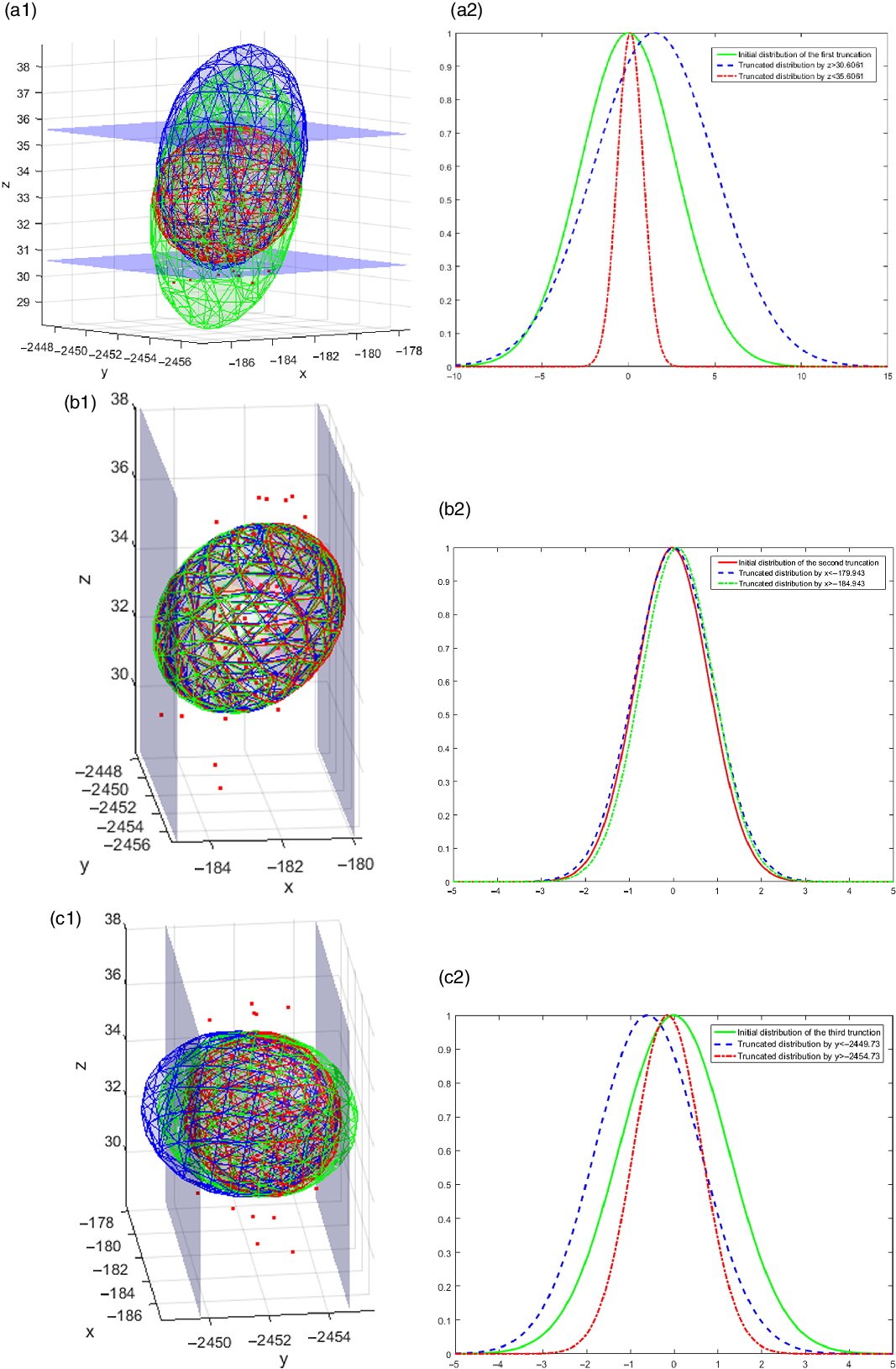
Figure 13. Distribution truncation process (unit:mm).
The trajectory is repeated for 100 times, while the high-accuracy optical gratings were used to measure the joint positions and the end position of the manipulator was got by forward kinematics. The recorded traces, together with the simulation results, were superimposed on the simulation system, as shown in Fig. 10. From the comparison results of experiment and simulation, the real end effector traces of the manipulator have the same trend and are particularly close. The distribution and its real experiment trajectories of an average PBVS visual servo method are shown in Fig. 11. By comparing Fig. 10 with Fig. 11, it can be find that the error range of the PBVS visual servo method which do not include nondetermination theory expends since the motion error and visual measurement error accumulates. But when the nondetermined trajectory planning method with system uncertainties was used, the manipulator can choose the best trajectory that can give the manipulator better feedback and motion features than the others. And then the error distribution of the end effector narrows.
With the algorithm proposed in this paper, the covariance matrix that represents the error distribution at the end of the trajectory is [0.9198, 0.0921, 0.5957; 0.0921, 1.2549, 0.1591; 0.5957, 0.1591, 2.7584]. As shown in Fig. 12, the green ellipsoid. With the method proposed in Section 3.2, the covariance matrix of estimated errors is transformed into the green ellipsoid as shown in Fig. 12. Since the capture system is compliant, it has a tolerance range in centimeters. The tolerance is 179.943< X < 184.943, 2449.73 < Y < 2454.73 and 30.6061 < Z < 35.6061, which can be seen as a cube surrounded six constraint planes as the blue planes simulate shown in Fig.12. The final truncated distribution whose geometric space do not interface with the constraint planes is shown as the red ellipsoid in Fig. 12. From the initial green distribution to the red distribution, the calculation process is shown in Fig. 13. The whole calculation process is divided into 6 steps, and the method proposed in 3.3 is used repeatedly in each step. The error distribution of the previous step and the current constraint are applied to calculate the new distribution satisfying the constraint.
The final error distribution that satisfies all the constraints is the final capture probability. The probability that the end effector capture the object is 81.957%. According to the actual measurement results, the number of times the end of the manipulator reaches the target area is 86, indicating that the probability of successfully capturing the target is 86%. Thus, it proofs that the results of the simulations and experiments are very close.
5. Conclusions
This paper presents an intelligent trajectory planning method that added on the basis of the classical PBVS visual servo method which can reasonably analyze the probability of success. In this method, the motion error and visual sensing error are integrated into the system model, and the iteration and reasonable estimation of trajectory are realized by means of Bayesian theory and linear quadratic optimal control. The advantage of this method of estimation is that it is not qualitative but quantitative. Compared with the classical PBVS method, the effectiveness and practicability of the proposed method are proved.
There are many more practical applications for the approach proposed in this paper. For example, in unmanned circumstance, such as the lunar soil sampling manipulator, can calculate and evaluate the sampling accuracy of the target location in real time according to the method in this paper. Selecting the target location with the highest probability of success can be more efficient and save energy. In addition, RRT and other algorithms can be used to plan many trajectories in the capture of specific targets. By the evaluation algorithm in this paper, the trajectory with higher success probability is selected as the predefined trajectory, which can improve the operation success probability. Especially for the space manipulator system, the huge temperature fluctuation and difficult heat dissipation conditions limit the choice of joint sensors, and the motion accuracy of the manipulator is much lower than that of the industrial manipulator on the ground. Therefore, the method in this paper is particularly applicable under this working condition. This method is also applicable to the optimal motion decision of deep-sea underwater manipulator and manipulator under strong electromagnetic interference.
The key of this method is to understand the motion error and sensing error of the system itself. The more accurate the setting of these two kinds of errors, the higher the fit between the nondeterministic system model and the reality will be, and then the more accurate the estimate of the ultimate probability of success.
In the future, the related methods will be applied to real-time decision making. In real-time applications, the verification method and dynamic characteristics of the algorithm need to be further studied.
Acknowledgements
The authors are grateful to be supported by the Natural Science Foundation of Liaoning Province (2019-ZD-0663), China Postdoctoral Science Foundation (2019M651145) and the State Key Laboratory of Robotics (2019-O21).
Availability of data and material
We declared that materials described in the manuscript, including all relevant raw data, will be freely available to any scientist wishing to use them for noncommercial purposes, without breaching participant confidentiality.
Conflicts of interest
The authors declare no competing financial interests.
Data availability statement
The data used to support the findings of this study are included within the article.